R E S E A R C H
Open Access
Generating nonclassical quantum input
field states with modulating filters
John E Gough
1*and Guofeng Zhang
2*Correspondence: [email protected] 1Department of Physics, Aberystwyth University, Aberystwyth, Wales SY23 2BZ, UK Full list of author information is available at the end of the article
Abstract
We give explicit constructions of quantum dynamical filters which generate
nonclassical states (coherent states, cat states, shaped single and multi-photon states) of quantum optical fields as inputs to general quantum Markov systems. The filters will be quantum harmonic oscillators damped by the input fields, and we exploit the fact that the cascaded filter and system will have a Lindbladian that is naturally Wick-ordered in the filter modes. In particular the initialization of the modulating filter will determine the signal state generated.
Keywords: quantum modulating filter; nonclassical states; measurement filtering
1 Introduction
There has been considerable progress in the generation of nonclassical states of light such as shaped single photons [–], cat states [–], etc., and this has been proposed for several quantum technologies [–]. Here we propose the use of quantum mechanical modu-lating filters prepared in nonclassical states which serve to generate nonclassical quantum noise output from vacuum input, and that may then be used to drive an open quantum system. The effect, after tracing out the modulator, is equivalent to driving the system by an input field in a nonclassical state, see Figure .
Historical, the concept of coloring white noises has enjoyed much application in con-trol engineering, and in particular signal processing. A white noise input, say correspond-ing to the derivative of a Wiener processB(t), may be converted into a colored process Y(t) =h(t–s)dB(s) wherehis a causal kernel function. In practice this convolution may be physically implementable by passing the input through a dynamical system, such as an electronic circuit, an obtainingY as output. The resulting output will have a nonflat spectrumSY(ω)≡ |H(ω)|, whereH(ω) is the Fourier transform of the kernelh, see for instance []. However, the concept is still useful as a theoretical construct in modelling systems driven by colored noise, as it allows an extended model with a white noise input. The idea has been extended to quantum systems, and at its simplest corresponds to cascading an ancillary system (the filter) in front of the system, a concept going back to Carmichael, []. A systematic study of quantum coloring filters was initiated in [] by one of the authors. More recently, finite-level ancillas were proposed to generate multi-photon states for quantum input processes []. In this setting, the dynamical and filtering equations took on a matrix form determined by the ancilla space. However, due to the
Figure 1 System with nonclassical input; a coloring filter (modulator) is used to convert vacuum noise input into a desired nonclassical input.Tracing out the modulating filter leads to the same master equation.
choice of couplings (raising and lowering of the ancilla levels) the class of multi-photon states obtained had a chronological ordering property of the photon one-particle states which was not the intended form of the multi-photon state. Or alternative here is to use linear quantum dynamical models as ancilla. We should also mention recent work of Xue et al.[] who have treated the Belavkin filtering problem for Ornstein-Uhlenbeck noise input: this input may be readily modelled as output of a linear system such as a cavity mode driven by white noise quantum input processes.
Notations Denote byFnthe span of all symmetrized vectors of the formf ˆ⊗ ··· ˆ⊗fn=
n!
σfσ()⊗ · · · ⊗fσ(n)wheref, . . . ,fnlie in a one-particle Hilbert spaceV, and the sum is over all permutationsσ of thenindices. The Boson Fock space overVis then the direct sumF =∞n=Fn, withFspanned by thevacuum vector|vac.
The creation, annihilation and conservation operators are then given by (fjindicating the omission of termfj)
B(g)∗f ˆ⊗ ··· ˆ⊗fn=
√
n+ g ˆ⊗f ˆ⊗ ··· ˆ⊗fn, B(g)f ˆ⊗ ··· ˆ⊗fn=
√
n n
j=
g|fjf ˆ⊗ ··· ˆ⊗fj ˆ⊗ ··· ˆ⊗fn,
(T)f ˆ⊗ ··· ˆ⊗fn= n
j=
f ˆ⊗ ··· ˆ⊗(Tfj) ˆ⊗ ··· ˆ⊗fn,
and they mapFntoFn+,Fn–andFnrespectively.
Given a complete orthonormal basis{e,e, . . .}forV, we obtain a complete orthonormal
basis forF by setting
|n=
n! n!n!· · ·
k e⊗nk
k ≡ ∞
k=
√
where n = (n,n, . . .) is a sequence of occupation numbers andn=
knk. The state|n corresponds to havingnkphotons in the stateekfor eachk.
For V =L[,∞), the space of square-integrable functions ξ(t) in t≥, we
intro-duce the annihilation processBt=B(χ[,t]) whereχ[,t] is the function equal to unity on
the interval tot, and zero otherwise. The It¯o differentialdBt has the actiondBt|n=
∞
k=
√
nk|n, . . . ,nk– , . . .ek(t)dt, where, for convenience, we may assume an orthonor-mal basis of continuous test functionsek. For nonorthonormal states we have
dBtf ˆ⊗ ··· ˆ⊗fn=
√
n
j
f ˆ⊗ ··· ˆ⊗fj ˆ⊗ ··· ˆ⊗fnfj(t)dt.
For convenience we consider a single quantum input process.
Now fix a quantum mechanical system with Hilbert spaceh, called theinitial space,
then an open system is described by the triple of operatorsG∼(S,L,H) onh- withS
the unitaryscattering matrix,Lthecollapse, or coupling, operatorandHtheHamiltonian - which fixes the open dynamical unitary evolutionU(t) onh⊗Fas the solution to the
quantum stochastic differential equation []
dUt=
(S–I)⊗dt+L⊗dB∗t –L∗S⊗dBt–
L
∗L+iH⊗dtU
t ()
and in the Heisenberg picture we setjt(X) =Ut∗X⊗IUtso that djt(X) =jt(LX)⊗dt+jt(LX)⊗dB∗t
+jt(LX)⊗dBt+jt(LX)⊗dt, ()
where we have the Evans-Hudson super-operators []
LX=
L
∗[X,L] +
L∗,XL–i[X,H],
LX=S∗[X,H], LX=
L∗,XS,
LX=S∗XS–X.
Theoutput processesare given by the formula
Boutt =U∗(t)B(t)U(t), ()
and we havedBout
t =jt(S)dBt+jt(L)dt.
Finally we recall that there is the natural factorizationF=F–t ⊗F+t of the Fock space into past and future Fock spaces for eacht> [].
Definition (from []) An operator on a tensor producth⊗his the ampliation of an
operatorXonhif it takes the formX⊗I. A quantum stochastic process (X(t))t≥is
adapted if, for eacht> , it is the ampliation of an operator on the past spaceh⊗F–t to the full spaceh⊗F.
The unitary evolution process (U(t))t≥is adapted, as will be the Heisenberg dynamical
process (jt(X))t≥, for each initial choice of operatorX. The following formula will be used
Lemma Let(X(t))t≥be a quantum stochastic integral process of the form
X(t) =X⊗IF+ t
x(s)ds+x(s)dB∗s+x(s)dBs+x(s)ds
, ()
where the(xαβ(t))t≥are adapted processes.Then
dU∗(t)X(t)U(t)=U∗(t)L(X) +x(t) +L∗x+xL+xL
dt
+L(X) +S∗x(t) +S∗xL
dB∗t
+L(X) +x(t)S+L∗xS
dBt
+L(X) +S∗x(t)S
dt
U(t). ()
The proof is a routine application of the quantum stochastic calculus []. We note that if we set the (xαβ(t))t≥equal to zero then we recover the standard Lindblad-Heisenberg
equations of motion forU∗(t)(X⊗IF)U(t): that is the noisy dynamics of the system
ob-servable with initial valueX. Conversely settingX= and taking the (xαβ(t))t≥to be
constants leads to the input-output relation. Equation () therefore contains general in-formation about evolution of both system observables and field observables.
2 Modulating filter
Our strategy is to employ a modulating filterMto process vacuum input and to feed this forward to the system. In principle, the modulator and system are run in series as a single Markov component driven by vacuum input, as in Figure . Tracing out the modulator de-grees of freedom leads to an effective model which leads to the same statistical model as a nonvacuum input to the system. We shall show below how to realize different nonclassical driving fields in this way. In our proposal we consider a linear passive system as modulator: physically corresponding to modes in a cavity. The choice of (time-dependent) coupling operators describing the modulator will be important in shaping the output, however, in this set-up the crucial element determining nonvacuum statistics will be the initial state φ∈hMof the modulator.
We consider our systemG∼(S,L,H) which is driven by the output of a modulatorM∼ (I,LM,HM) which itself is driven by vacuum noise. The modulator and system in series is described by the series product [, ] on the joint spacehM⊗hG
G=GM∼I⊗S,I⊗L+LM⊗S,I⊗H+HM⊗I+Im
LM⊗L∗S
. ()
Let us denote byUtthe joint unitary generated byG. This is a unitary adapted process with initial spaceh=hM⊗hG.
Definition LetGdetermine an open quantum system and let∈Fbe a state of the input field. A modulatorMwith initial stateφand vacuum input is said to replicate the
open system if we have (with|=|φ⊗ψ⊗vac)
|U(t)∗
IM⊗X(t)U(t)|=ψ⊗|U(t)∗X(t)U(t)|ψ⊗ ()
2.1 The cascaded Lindbladian
The total Lindbladian corresponding toGis
L(A⊗X) =LM(A)⊗X+
μ=,
ν=,
L∗MμA[LM]ν⊗LμνX, ()
whereLMA=[LM∗ ,A]LM+L∗M[A,LM] –i[A,HM] is the modulator Lindbladian.
2.2 Oscillator mode modulators
Our interest will be in modulators that are linear passive systems. To this end, we begin with the simplest model of a single Boson modea(say a cavity mode) as modulator, and set
HM=ω(t)a∗a,LM=λ(t)a. ()
For simplicity we shall takeω(t)≡ andλto be a complex-valued time-dependent damp-ing parameter.
A key feature of equation () whenLM=λ(t)ais that theaanda∗appear inWick ordered formaboutA. We now exploit this property.
To compute expectations, we introduce the operator
atUt∗(a⊗I)Ut
and observe thatdat= –z(t)atdt–λ(t)∗dBt where we have the complex dampingz(t) =
|λ(t)|+iω(t). The solution to this is the operator at=e–ζ(t)a–
t
λ(s)∗eζ(s)–ζ(t)dBs
withζ(t) =tz(s)ds.
Setting|=|φ⊗ψ⊗vac, we have
d
dt|U(t) ∗(I
M⊗X⊗IF)U(t)|
=
μ,ν=,
|U(t)∗
λ(t)∗a∗μλ(t)aν⊗LμνXU(t)|
=
μ,ν=,
|
λ(t)∗a∗tμU(t)∗(IM⊗LμνX)U(t)
λ(t)at
ν
|
=
μ,ν=,
ξ(t)∗μξ(t)ν[a]μ
Ut∗(I⊗LμνX⊗I)Ut[a]ν
, ()
where
2.3 Generating shaped 1-photon fields
The problem we ideally wish to solve is how to generate a desired pulse shape ξ, and this means choosing the correct λ. It will be required that ξ be normalized, that is,
∞
|ξ(t)|dt= . Now let us setw(t) =exp{– t
|λ(s)|ds}, then
d
dtw(t) = –λ(t)
exp
–
t
λ(s)ds
≡–ξ(t)
and, imposing the correct initial conditionw() = , we obtain
w(t)≡
∞
t
ξ(s)ds. ()
Again takingω(t)≡ for simplicity, we findz(t)≡ |λ(t)|, real-valued. As we are given
ξ normalized, we see that the appropriate choice forλis
λ(t) = √
w(t)ξ(t), ()
withwgiven by (). An additional phase term will appear if we haveω(t) nonzero.
2.4 Replicating nonvacuum input
LetG∼(S,L,H) andM∼(IM,λa,ωa∗a) and let (X(t))t≥be a quantum stochastic integral
process onhG⊗F, as in () then we may generalize () to get d
dt|U(t) ∗I
M⊗X(t)U(t)|
=|U(t)∗IM⊗
L(X) +x+L∗x+xL+L∗xLU(t)|
+ξ∗|a∗U(t)∗IM⊗
L(X) +S∗x+S∗xLU(t)|
+ξ|U(t)∗IM⊗
L(X) +xS+L∗xSU(t)a|
+ξ∗ξ|a∗U(t)∗IM⊗
L(X) +S∗xSU(t)a|. ()
This follows from () where we replace theSandLwith the cascaded operatorsIM⊗S andIM⊗L+λa⊗S.
For the modulator to replicate the dynamics with nonvacuum state, the derivative
d
dtψ⊗|U(t)
∗X(t)U(t)|ψ
⊗
must equal the corresponding expression () for any quantum stochastic integral process X(t) on the Hilbert spacehG⊗F. We may use () to show directly that this is computed from the following expectation
dψ⊗|U(t)∗X(t)U(t)|ψ⊗
=ψ⊗|U∗(t)
L(X) +x(t) +L∗x+xL+xL
dt
+L(X) +S∗x(t) +S∗xL
+L(X) +x(t)S+L∗xS
dBt
+L(X) +S∗x(t)S
dt
U(t)|ψ⊗. ()
The modulator therefore replicates the nonvacuum input model.
2.5 Replicating coherent states
As a simple illustration let us show how we may construct a modulator that replicates a coherent state|βfor the input field, whereβ(t) is a square integrable function of time t≥. Note that
dBt|β=β(t)|β.
We see that the equations () and () have structural similarities, and a first guess for the initial state of the modulator is another coherent state
φ=|α,
whereα∈Cis the intensity of the mode coherent state. In this caseaφ=αφand ()
and () coincide for the choice
ξ(t)α≡β(t). ()
We therefore get the following result.
Theorem The quantum open system G∼(S,L,H)driven by input in the continuous-variable coherent state=|βis replicated by the single mode modulator of the linear form M∼(IM,λa,ωa∗a)with the initial stateφ=|αfor the modulator and withλ(t)and
ω(t)chosen so that()holds.
3 Replicating multi-photon input 3.1 Fock state input fields
The state of a single mode quantum input field corresponding tonquanta with the same (normalized) one-particle test functionξ∈L[,∞) is
ξ⊗n=√ n!B
∗(ξ)n|vac.
We see that the annihilator acts on such states as
dBtξ⊗n=
√
nξ(t)ξ⊗n–dt.
One of the consequences of this comes when we try and compute expectations of the form
ψ⊗ξ⊗nx(t)dBtψ⊗ξ⊗n
which then equals
√
nξ(t)ψ⊗ξ⊗nx(t)ψ⊗ξ⊗n–
which is a matrix element between annphoton state and ann– photon state. This feature will be typical, and so it is convenient to introduce general matrix elements
Mnl,nr t (X) =
ψ⊗ξ⊗nlU(t)∗X(t)U(t)ψ⊗ξ⊗nr
,
wheneverX(t) is a quantum stochastic integral andnl,nr≥. We setMntl,nr(X)≡ if we ever havenlornrnegative.
TakingXto have the form (), we see that () leads to
d dtM
nl,nr
t (X) =M nl,nr t
L(X) +x(t) +L∗x+xL+xL
+√nξ∗(t)Mnl–,nr t
L(X) +S∗x(t) +S∗xL
+√nξ(t)Mnl,nr– t
L(X) +x(t)S+L∗xS
+nξ(t)Mnl–,nr–
t
L(X) +S∗x(t)S
. ()
We note the hierarchical nature of these equations with the rate of change ofMnl,nr t (X) depending on lower order matrix elements.
Now let us introduce the single mode modulator, and let|nbe the number states for the oscillator mode (n= , , , . . .). We may similarly introduce the matrix elements
Mnl,nr
t (X) =nl⊗ψ⊗vac|U(t)∗
IM⊗X(t)
U(t)|nr⊗ψ⊗vac,
withnl,nr≥, andMtnl,nr(X) = if either index is negative. From (), we see that
d dtM
nl,nr
t (X) =M nl,nr t
L(X) +x(t) +L∗x+xL+xL
+√nξ∗(t)Mnl–,nr t
L(X) +S∗x(t) +S∗xL
+√nξ(t)Mnl,nr– t
L(X) +x(t)S+L∗xS
+nξ(t)Mnl–,nr– t
L(X) +S∗x(t)S
. ()
It follows that the systems of equations () and () are identical, and so we identify
Mnl,nr
t (X)≡M nl,nr t (X)
for all quantum stochastic integral processX(t) on the joint system and field. We summa-rize the result as follows.
Theorem The quantum open system G∼(S,L,H) driven by input in the nonclassi-cal state =ξ⊗n is replicated by the single mode modulator of the linear form M∼ (IM,λ(t)a,ω(t)a∗a)with the initial stateφ=|nfor the modulator and withλ(t)andω(t)
3.2 General multi-photon input fields
To generate multi-photon input field state (assumed normalized)
(n) = N
k=
ξ⊗nk
k , ()
where now theξkare distinct, we need a multimode cavity with several independent pho-ton modesa, . . . ,aN. The coupling operator may now be extended to
LM=
k
λk(t)ak.
It is convenient to introduce the vectors
ξ(t) =ξ(t), . . . ,ξN(t)
,
λ(t) =λ(t), . . . ,λN(t)
,
a=
⎡ ⎢ ⎢ ⎣
a
.. . aN
⎤ ⎥ ⎥ ⎦
so thatLM≡λ(t)a. We consider the vector of time-evolved modesat=U˜t∗aUtand from the It¯o rules, we find
da˜t=A(t)a˜tdt=λ(t)†dBt,
whereA(t) in the time-dependentN×Nmatrix with entries
Ajk(t) = – λ
∗
j(t)λk(t) –iωkδjk.
The solution is
˜
at=(t)a–(t)
t
(s)–λ(s)†dBs,
which is given in terms of the transition matrix(t) satisfying
d
dt(t) =A(t)(t), () =IN.
We then obtain the following vectorial generalization of ()
d
dt|U(t) ∗I
M⊗X(t)U(t)|
=|U(t)∗IM⊗
L(X) +x+L∗x+xL+L∗xLU(t)|
+|a∗(t)†λ(t)∗U(t)∗IM⊗
L(X) +S∗x+S∗xLU(t)|
+|U(t)∗IM⊗
L(X) +xS+L∗xSU(t)λ(t)(t)a|
+|a∗(t)†λ(t)∗U(t)∗IM⊗
Evidently, to get a prescribed set of pulsesξ(t), we need to chooseλ(t) and theωk(t)’s such that
ξ(t) =λ(t)(t). ()
In general this is a difficult problem to solve, but for weak pulses the Magnus expansion [] may offer a way to construct approximations. The set of functions ξk that may be constructed in this way is expected to be fully general given the freedom of choosing the λkandωk, [].
We now prepare the modulator in the initial state
φ=|n=|n, . . . ,nN, ()
where we havenkquanta in thekth cavity mode. This time we consider the family of expectations
Mnl,nr
t (X) =nl⊗ψ⊗vac|Ut∗
IM⊗X(t)Ut|nr⊗ψ⊗vac,
for occupation sequences nl= (nk,l) and nr= (nk,r).
d dtM
nl,nr t (X)
=Mnl,nr t
L(X) +x(t) +L∗x+xL+xL
+ N
k=
√
nk,lξk(t)∗M nl–δk,nr t
L(X) +S∗x(t) +S∗xL
+ N
j=
√
nj,rξj(t)M nl,nr–δj t
L(X) +x(t)S+L∗xS
+ N
k=
N
j=
√
nk,lξk(t)∗√nj,rξj(t)M
nl–δk,nr–δj t
L(X) +S∗x(t)S
, ()
where nowδk is the occupation sequence wherenk= and all other terms are zero. We add sequences together in the obvious way so that n –μδkequals n ifμ= , and (n, . . . ,
nk– , . . . ,nN) ifμ= .
By similar arguments to before, we see that system of expectations
Mnl,nr t (X) =
ψ⊗(nl)Ut∗X(t)Utψ⊗(nr)
,
generate the same system of as theMnl,nr
t (X) and so may be equated. We have therefore established that
Theorem The quantum open system G∼(S,L,H)driven by input in the nonclassical state (n) =!Nk=ξ⊗nk
k is replicated by the N mode modulator of the linear form M∼ (IM,kλk(t)a,kωk(t)a∗kak)with the initial stateφ=|n for the modulator and with
4 Superposition principles
We now make a basic observation.
Principle of Superimposed models For a fixed modulator M - that is, a quantum open system with definite(IM,LM,HM)- suppose that initial states|φA,|φB, . . .replicate
|A,|B, . . .respectively and are compatible in so far as
φA⊗ψ⊗vacU(t)∗
IM⊗X(t)U(t)φB⊗ψ⊗vac
=ψ⊗AU(t)∗X(t)U(t)ψ⊗B
()
for each pair A,B.Then if the modulator is prepared in a normalized superposition|φ=
cA|φA+cB|φB+· · · replicates the nonclassical state|=cA|A+cB|B+· · ·. This follows automatically from the bra-ket structure of the matrix elements.
4.1 Replicating cat states
We would like to generate a superposition of coherent states (cat states [–])
=
k γk|βk,
withk,lγk∗γleβk,βl= for normalization. It is easy to see that pairs of coherent states are compatible in the sense of the superposition principle.
We know that the modulator (with fixed structureLM=λ(t)a,HM=ω(t)a∗a) prepared in coherent state|αkwill replicate the open system with coherent state|βkfor the
βk(t) =ξ(t)αk. ()
The principle of superposition therefore implies that the initial statekγk|βkfor the modulator will then replicate the cat state=kγk|βk. Note that theβk that may be generated this way must take the form (). This is somewhat restrictive since we cannot obtain independent pulse, only pulse which differ by the scale factorsαk. However this already gives a wide class of cat states for practical purposes.
5 Conclusion
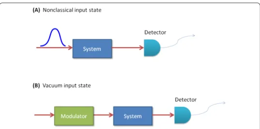
Figure 2 Continuous measurement of (A) the output of a system driven by nonclassical noise, and (B) and equivalent model from a modulated vacuum noise.
and noise model in a strong sense: that is we show that general quantum stochastic in-tegral processes on the system plus noise space have identical averages in the original model with nonclassical input and in the modulated model with vacuum input. This in particular establishes equivalence of the system dynamics (effectively the same Ehrenfest equations for system observables) as well as equivalence of the outputs. The latter point is of major importance with regards to quantum trajectories (quantum filtering theory) since whenever we perform continuous measurements (e.g., quadrature homodyning, or photon counting), [–] on the output we have that the measurement processes of the original model and the modulate model are statistically identical. See Figure .
As a conceptual tool, this opens up the prospect of extending known results on quantum trajectories for vacuum inputs to models with nonclassical inputs. One such feature which we will address in a future publication is the issue of filter convergence, that is, when does the estimated conditional density operator converge to the true conditional density oper-ator when one starts with the wrong initial stateψfor the system - this has been treated
for vacuum inputs [], but is largely unknown in the case of nonclassical inputs.
Competing interests
The authors declare that they have no competing interests.
Authors’ contributions
All authors contributed equally to the writing of this paper. All authors read and approved the final manuscript.
Author details
1Department of Physics, Aberystwyth University, Aberystwyth, Wales SY23 2BZ, UK.2Department of Applied
Mathematics, The Hong Kong Polytechnic University, Hong Kong, ACT, 0200, China.
Acknowledgements
The authors acknowledge support through the Royal Academy of Engineering UK and China scheme, and National Natural Science Foundation of China (NSFC) grant (Nos. 61374057) and a Hong Kong RGC grant (No. 531213).
Received: 14 January 2015 Accepted: 1 June 2015
References
1. Lvovsky AI, Hansen H, Aichele T, Benson O, Mlynek J, Schiller S. Phys Rev Lett. 2001;87:050402.
2. Pechal M, Huthmacher L, Eichler C, Zeytino ˘glu S, Abdumalikov AA Jr, Berger S, Wallraff A, Filipp S. Phys Rev X. 2014;4:041010.
4. Yuan Z, Kardynal BE, Stevenson RM, Shields AJ, Lobo CJ, Cooper K, Beattie NS, Ritchie DA, Pepper M. Science. 2002;295:102.
5. McKeever J, Boca A, Boozer AD, Miller R, Buck JR, Kuzmich A, Kimble HJ. Science. 2004;303:1992. 6. Eichler C, Bozyigit D, Lang C, Steffen L, Fink J, Wallraff A. Phys Rev Lett. 2011;106:220503.
7. Neergaard-Nielsen JS, Melholt Nielsen B, Hettich C, Mølmer K, Polzik ES. Phys Rev Lett. 2006;97:083604. 8. Ourjoumtsev A, Tualle-Brouri R, Laurat J, Grangier P. Science. 2006;312:83.
9. Ourjoumtsev A, Jeong H, Tualle-Brouri R, Grangier P. Nature. 2007;448:784.
10. Houck AA, Schuster I, Gambetta JM, Schreier JA, Johnson BR, Chow JM, Frunzio L, Majer J, Devoret MH, Girvin SM, Schoelkopf JM. Nature. 2006;449:328.
11. Ralph TC, Gilchrist A, Milburn GJ. Phys Rev A. 2003;68:042319. 12. Gisin N, Ribordy G, Tittel W, Zbinden H. Rev Mod Phys. 2002;74:145. 13. Anderson BDO, Moore JB. Optimal filtering. New York: Dover; 2005.
14. Carmichael HJ. An open systems approach to quantum optics. Lectures presented at the Universite Libre de Bruxelles, October 28 to November 4, 1991. Lecture notes in physics. vol. 18. 1994.
15. Gough JE, James MR, Nurdin HI, Combes J. Phys Rev A. 2012;86:043819. 16. Gough JE, James MR, Nurdin HI. New J Phys. 2014;16:075008.
17. Xue S, James MR, Shabani A, Ugrinovskii V, Petersen IR. Submitted to the 54th IEEE conference on decision and control. arXiv:1503.07999.
18. Cirac JI, Zoller P, Kimble HJ, Mabuchi H. Phys Rev Lett. 1997;78:3221. 19. Hudson RL, Parthasarathy KR. Commun Math Phys. 1984;93:301-23.
20. Evans MP, Hudson RL. In: Accardi L, von Waldenfels W, editors. Quantum Probability & Applications, Volume III. Lecture Notes in Mathematics. vol. 1303. Heidelberg: Springer; 1988. p. 69-88.
21. Gough JE, James MR. Commun Math Phys. 2009;287:1109-32. 22. Gough JE, James MR. IEEE Trans Autom Control. 2009;54:2530. 23. Magnus W. Commun Pure Appl Math. 1954;7:649-73. 24. Wei J. J Math Phys. 1963;4:1337-41.
25. Belavkin VP. Radiotec Electron. 1980;25:1445-53. 26. Belavkin VP. J Multivar Anal. 1992;42:171-201. 27. Wiseman HM, Milburn GJ. Phys Rev Lett. 1993;70(5):548. 28. Wiseman HM, Milburn GJ. Phys Rev A. 1993;47(1):642.