Improvement of the Deep Forest Classifier by a Set of Neural Networks
Lev V. Utkin and Kirill D. Zhuk
Peter the Great, St.Petersburg Polytechnic University (SPbPU), Russia E-mail: [email protected]
Keywords:classification, random forest, decision tree, deep learning, neural network, class probability distribution
Received:April 1, 2019
A Neural Random Forest (NeuRF) and a Neural Deep Forest (NeuDF) as classification algorithms, which combine an ensemble of decision trees and neural networks, are proposed in the paper. The main idea underlying NeuRF is to combine the class probability distributions produced by decision trees by means of a set of neural networks with shared parameters. The networks are trained in accordance with a loss function which measures the classification error. Every neural network can be viewed as a non-linear function of probabilities of a class. NeuDF is a modification of the Deep Forest or gcForest proposed by Zhou and Feng, using NeuRFs. The numerical experiments illustrate the outperformance of NeuDF and show that the NeuRF is comparable with the random forest.
Povzetek: V povzetku sta predstavljena dva izvirna algoritma: nevronski nakljuˇcni gozdovi in nevronski globoki gozdovi.
1
Introduction
In spite of the intensive development of a huge number of various modern classification models, including the deep learning models, the ensemble methodology remains one of the most efficient approaches for solving machine learn-ing problems. The ensemble learnlearn-ing models are based on constructing multiple classifiers for training data and on aggregating their corresponding predictions in accordance with a certain rule. The final ensemble classifier is repre-sented as a weighted average of outputs of the base or weak classifiers. The weight of each classifier can be viewed as its contribution to the final decision. Several approaches use some functions that combine the outputs from all base classifiers instead of weighted averages. From a statisti-cal point of view, one of the ideas underlying the improve-ment of the classifier performance by means of the ensem-ble combinations is based on reduction of variance of the classification error [11]. This occurs because the usual ef-fect of ensemble averaging is the reduction of the variance of a set of classifiers.
Three main techniques of combining the classifiers can be pointed out [44]: bagging, stacking and boosting. Bag-ging [4] aims to improve accuracy by combining multi-ple classifiers. One of the most powerful bagging meth-ods is the random forest (RF) method [5], which uses a large number of individual decision trees in order to com-bine their predictions. Another technique for achieving the highest generalization accuracy in the framework of ensemble-based methods is stacking [41]. This technique is used to combine various classifiers by means of a meta-learner that takes into account which classifiers are reliable and which are not. The best known ensemble-based tech-nique is boosting which improves the performance of weak
classifiers by means of their combining into a single strong classifier. Both boosting and bagging techniques use voting for combining the classifiers. However, the voting mecha-nism is differently implemented. In particular, examples in bagging are chosen with equal probabilities. Boosting supposes to choose the examples with probabilities that are proportional to their weights [32].
There are several review papers devoted to various ap-proaches based on the combination of classifiers. A de-tailed analysis of many ensemble-based methods can be found in a review proposed by Ferreira and Figueiredo [14]. The review compares a huge number of modifications of boosting algorithms. One of the first books thoroughly studying combination rules for improving classification performance was written by Kuncheva [23]. An interesting review of ensemble-based methods is proposed by Polikar [30]. A nice review is presented by Wozniak et al. [42] A comprehensive analysis of combination algorithms and their application to machine learning approaches such as classification, regression, clusterization can be also found in a review paper written by Rokach [32]. We have to point out also other recent reviews [13, 19, 31, 43]. A detailed description and an exhaustive analysis of most ensemble-based models are given in Zhou’s book [44].
[2, 9, 15, 27, 33].
An interesting new ensemble-based method which can be viewed as a combination of several ensemble-based methods, including the RF and the stacking, is proposed by Zhou and Feng [45] and called the Deep Forest (DF) or gcForest. Its structure consists of layers similar to a multi-layer neural network structure, but each multi-layer in gcForest contains many RFs instead of neurons. gsForest can be regarded as an multi-layer ensemble of decision tree en-sembles. As pointed out by Zhou and Feng [45], gcForest is much easier to train and can perfectly work when there are only small-scale training data in contrast to deep neu-ral networks which require great effort in hyperparameter tuning and large-scale training data. A lot of numerical ex-periments provided by Zhou and Feng [45] illustrated that gcForest outperforms many well-known methods or is at least comparable with them.
Advantages of gcForest motivate us to modify it in or-der to improve its classification capability. Some im-provements have been proposed by Utkin and Ryabinin [37, 38, 39]. In particular, modifications of the DF for solving the weakly supervised and fully supervised met-ric learning problems were proposed in [39] and [37], re-spectively. A transfer learning model using the DF was presented in [38]. The main idea underlying the proposed modifications is to assign weights to decision trees in ev-ery RF in order to minimize the corresponding loss func-tions which depend on the problem solved. The weights are used to replace the standard averaging of the class proba-bilities for every instance and every decision tree with the weighted average. The weights are regarded as training pa-rameters which can be computed by solving the constrained quadratic optimization problems.
By introducing the tree weights, we simultaneously try to overcome another shortcoming of gcForest. It cannot be fully considered as an alternative to deep neural networks due to its uncontrollability in the sense of defining a goal in tasks different from the standard classification. One of the advantages of neural networks is the flexibility of specify-ing the error or loss function dependspecify-ing on the data process-ing task or a specific application. The loss function in the standard classification problem is determined by the dif-ference between a true class label of a training set element and a label computed by means of the forward propagation. The Euclidean distance between the input and output of the network is used in autoencoders. Various types of dis-tances between the probability distributions of the source and target data are used in transfer learning problems. The variety of error functions allows solving a lot of machine learning problems by specifying the required loss function. Therefore, another aim of the modifications is to modify gcForest in order to use different loss functions. We have to point out that the idea of weighting in RFs is also not new. Most weighting RF methods use weights of classes to deal with imbalanced datasets, for example, [10]. At the same time, there are a lot of publications devoted to more complex weight assignments to every tree. In
partic-ular, Li et al. [25] propose to assign weights to decision trees according to their classification ability. A similar ap-proach for weighting decision trees is presented by Kim et al. [20]. An interesting study of weighted voting methods in RFs is also given in [34]. The main difference of these methods from the proposed approach is that all the methods use some measures of the classification quality in order to assign the weights. Moreover, these measures are obtained on the basis of testing data. To the best of our knowledge, there are no methods which consider the weights as train-ing parameters. The proposed approach allows us to select a weighting assignment scheme in a flexible way by using different loss functions for optimization.
The approach using weights of decision trees for com-puting a target probability class vector for every RF have illustrated the outperformance in comparison with gcFor-est. However, it has some shortcomings. First, the number of weights is strongly depends on the number of decision trees in every RF. On the one hand, we increase the number of trees in order to increase the classification accuracy, but the large number of decision trees leads to the same large number of weights. As a result, the number of training pa-rameters is increased and the model may lead to overfitting. On the other hand, a reduction of decision trees may lead to a reduction of the classification accuracy. Second, the weighted average used for computing the RF probability class vector is a linear function of the weights. This fact significantly restricts a set of possible solutions and may make worse the classifier.
In order to overcome the above difficulties, we propose to use a neural network of a special form for computing the probability class vectors. The neural network plays a role of a non-linear analog of the linear function of weights. Of course, we do not have the weights of decision trees in the explicit form now. But we get a function which combines the probabilities of every class at the leaf nodes in order to obtain the RF probability class vector. In other words, the neural network plays a role of a non-linear function of weights. It should be noted that the proposed neural net-work is not standard because we have to identically process probabilities of every class. This implies that if the num-ber of classes is C, then we construct C identical neural networks with shared parameters. In particular, if a train-ing data have two classes, then the obtained neural network is very similar to the Siamese neural network [6] which has been widely used in many applications (see, for exam-ple, [1, 8, 17]). Outputs of all identical networks for every training instance form the corresponding probability class vector. In fact, the neural networks can be viewed as a non-linear alternative to the weighted sum of probabilities. In particular, this approach coincides with the approach us-ing the weighted averages when activation functions of all units in the neural networks are linear. The proposed com-binations of the neural network with the RF and the DF are called NeuRF and NeuDF, respectively.
constructing a denoising RF was proposed by Hibino et al. [16]. Another combination of the RF with the neural network was presented by Kontschieder et al. [21] where an ensemble of random trees is restructured as a collec-tion of random neural networks, which exhibits better gen-eralization performance. The authors of [21] introduced a soft differentiable decision function at the split nodes and a global loss function defined on a tree. Following this approach, several similar models were proposed in [3, 18, 35, 36, 40, 46]. Maji et al. [28] used a deep neural network for unsupervised learning followed by supervised learning of the deep neural network response using a RF.
In contrast to the above combinations of neural networks and RFs, in the presented paper, we incorporate the neural networks into the DF in order to correct and to control the class vectors at outputs of RFs. Our experiments demon-strate that NeuRF and NeuDF are competitive on many publicly available datasets.
2
A short introduction to deep
forests
One of the important peculiarities of gcForest is its cascade structure proposed by Zhou and Feng [45]. Every cascade is represented as an ensemble of decision tree forests. The cascade structure is a part of a total gcForest structure. It implements the idea of representation learning by means of the layer-by-layer processing of raw features. Each level of cascade structure receives feature information processed by its preceding level, and outputs its processing result to the next level. The architecture of the cascade proposed by Zhou and Feng [45] is shown in Fig. 1. It can be seen from the figure that each level of the cascade consists of several RFs which generate 3-dimensional class vectors concate-nated each other and with the original input. It should be noted that this structure of forests can be modified in or-der to improve the gcForest for a certain application. After the last level, we have the feature representation of the in-put feature vector, which can be classified in order to get the final prediction. The gcForest representational learning ability is enhanced by applying the second part of gcForest called as the so-called grained scanning. The multi-grained scanning structure uses sliding windows to scan the raw features. Its output is a set of feature vectors produced by sliding windows of multiple sizes. We mainly pay atten-tion to the first part of gcForest because our modificaatten-tion relates to the RFs.
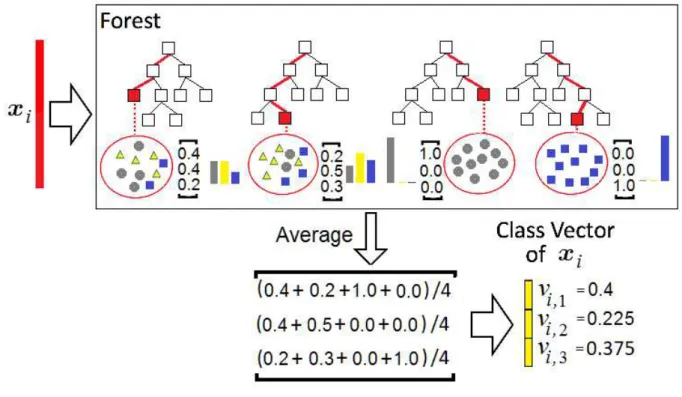
Given an instance, each forest produces an estimate of a class distribution by counting the percentage of different classes of examples at the leaf node where the concerned instance falls into, and then averaging across all trees in the same forest as it is schematically shown in Fig. 2. The class distribution forms a class vector, which is then con-catenated with the original vector to be input to the next level of cascade. The usage of the class vector as a re-sult of the RF classification is very similar to the idea
un-derlying the stacking algorithm [41] which trains the first-level learners using the original training dataset. Then the stacking algorithm generates a new dataset for training the second-level learner (meta-learner) such that the outputs of the first-level learners are regarded as input features for the second-level learner while the original labels are still re-garded as labels of the new training data. In contrast to the standard stacking algorithm, gcForest simultaneously uses the original vector and the class vectors (meta-learners) at the next level of cascade by means of their concatenation. This implies that the feature vector is enlarged after every cascade level. After the last level, we have the feature rep-resentation of the input feature vector, which can be clas-sified in order to get the final prediction. Zhou and Feng [45] propose to use different forests at every level in order to provide the diversity which is an important requirement for the RF construction.
It is interesting to note that the same architecture of the cascade forest was proposed by Miller et al. [29]. This architecture differs from gcForest in using only class vec-tors at the next cascade levels without concatenation with the original vector. Miller et al. [29] illustrated by numer-ical experiments that their approach is comparable to the approach [45]. We have to point out that the cascade struc-ture with neural networks without backpropagation instead of forests was proposed by Hettinger et al. [7].
3
Weighted averages in forests
One of the ways to improve gcForest is to assign weights to decision trees in every RF. The weights aim to correct the original averaging of class probability distributions over all decision trees in accordance with a predefined objective function. In the standard classification problem, the objec-tive function is the error function or the difference between class labels of training instances and values of the forest class probability distributions. In the metric learning prob-lem, the objective function is the distance between similar and dissimilar instances. Different machine learning prob-lems define the corresponding objective function and the corresponding weights of decision trees.
Our aim is to briefly consider the idea of the weighted average in order to propose the neural networks for pro-cessing the class probability distributions. Therefore, we will consider the standard classification problem for sim-plicity. The classification problem can be formally writ-ten as follows. Givenntraining data (examples, instances, patterns) S = {(x1, y1),(x2, y2), ...,(xn, yn)}, in which
xi ∈Rmrepresents a feature vector involvingmfeatures andyi ∈ {1, ..., C} represents the class of the associated
instances, the task of classification is to construct an ac-curate classifierc :Rm → {1, ..., C}that maximizes the
probability thatc(xi) =yifori= 1, ..., n.
A decision tree in every forest produces an estimate of the class probability distributionp= (p1, ..., pC)by
Figure 1: The architecture of the cascade forest [45].
at the leaf node where the concerned instance falls into. Then the class probabilities for every forest are computed by averaging all class probability distributionspacross all trees by taking into account the weights of the trees.
Suppose that all RF have the same numberTof decision trees, every cascade level containsM RFs, and the number of cascade levels isQ.
The objective function for computing optimal weights is defined as the Euclidean distance between the class vector and a vector such that its element with index yi is 1and
other elements are0. According to [45], the class distribu-tion forms a class vector which is then concatenated with the original vector to be input to the next level of the cas-cade. Suppose an origin vector isxi, and thep
(t,k,q)
i,c is the
probability of classcfor an instancexiproduced by thet
-th tree from -thek-th forest at the cascade levelq. Since we consider a single RF at some cascade level, then we omit indices kandq corresponding to the forest and the level, respectively. Let us also introduce the notation
pi,c=
p(i,ct), t= 1, ..., T,
w= (wt, t= 1, ..., T),
vi= (vi,c, c= 1, ..., C).
Herewtis the weight of thet-th tree in the considered
forest. Suppose that1is a vector havingT unit elements. Then thec-th elementvi,cof the class vector produced by
the considered forest for the instance xi is determined in
gcForest as
vi,c=T−1·pi,c·1T (1)
The weighted average of the class probability distribu-tions leads to the following class vectors
vi,c=pi,c·w.
It follows from the above that gcForest is a special case of the weighting scheme when all weights are1/T.
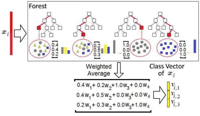
An illustration of the weighted averaging is shown in Fig. 3, where we partly modify a picture from [45] in order to show how elements of the class vector are derived as a simple weighted sum. One can see from Fig. 3 that the augmented featuresvi,c,c= 1, ..., C, corresponding to the
q-th forest are obtained as weighted sums, i.e., there hold
vi,1= 0.4w1+ 0.2w2+ 1.0w3+ 0.0w4, vi,2= 0.4w1+ 0.5w2+ 0.0w3+ 0.0w4, vi,3= 0.2w1+ 0.3w2+ 0.0w3+ 1.0w4.
The weights are restricted by the following obvious con-ditions:
w·1T= 1, wt≥0, t= 1, ..., T. (2)
Now we can write the objective function for computing optimal weights:
J(w) = min
w n
X
i=1
kvi−oik
2
2+λR(w).
HereR(w)is a regularization term,λis a hyper-parameter which controls the strength of the regularization, oi =
(0, ...,0,1c,0, ...,0).
Figure 2: An illustration of the class vector generation by using average of the tree probability class vectors.
4
Neural networks as a function of
class probabilities
Let us return to the weighted averaging. The valuevi,ccan
be represented as a function f of probabilities pi,c, i.e.,
vi,c =f(pi,c). It is important to point out that the function
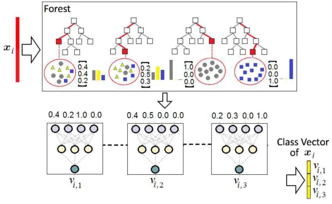
f does not depend on the classc. At the same time, it is identical for all classes. Suppose now that the functionf is not linear and is implemented by using the neural net-work. This implies that, for every class, we have to identi-cally transform the vectorpi,cin order to get the vectorvi
for every forest. It can be done by usingCidentical neu-ral networks with shared parameters. The input of thec-th network is the vectorpi,c of the lengthT. The output of
thec-th network is expected to be1if the class label of the i-th instance coincides with the number of the network, i.e., if the conditionyi=cis valid, otherwise the output is
ex-pected to be0. The networks are trained on the basis of sets of vectorspi,cobtained for every training example(xi, yi),
i = 1, ..., n. The condition for training is that parameters of all networks have to be identical, i.e., the networks are implemented with shared parameters. This implies that that all networks are trained simultaneously.
Fig. 4 illustrates the use of identical neural networks with shared parameters for computing the class vectors. It can be seen from the picture that the input vector for the first neural network consists of first class probabilities of class probability distributions produced by all trees, i.e., it is the vector (0.4,0.2,1.0,0.0). The input vector for the second neural network consists of probabilities of the
sec-ond class, i.e., it is the vector (0.4,0.5,0,0). The same can be written for the third network input vector. In other words, the k-th network uses all probabilities of thek-th class. In the case of two classes, we have the standard Siamese neural network [6].
It should be noted that one network, say the last one, is superfluous because theC-th element of the vectorvican
be obtained from its other elements under condition that the sum of all probabilities should be equal to1. However, we use it in order to compensate a possible bias of probabili-ties.
A total algorithm of training the DF is given as Algo-rithm 1.
Having the trained NeuDF, we can make decision about the class of a new examplex. By using the trained decision trees and the neural networks, the vectorxis augmented at each level. Finally, we get the vectorviof augmented
fea-tures after theQ-th level of the forest cascade correspond-ing to the original examplex. The examplexbelongs to the classc, if the sum of thec-th elements of all vectorsvi
obtained for all RFs and all cascades (the total number of vectors isPQ
q=1Mq) is maximal.
neu-Figure 3: An illustration of the class vector generation taking into account the weights.
Algorithm 1A total algorithm for training the NeuDF Require: Training setS ={(xi, yi), i = 1, ..., n},xi ∈
Rm,yi ∈ {1, ..., C}; number of levelsQ; number of
forests at theq-th levelMq
Ensure: wfor everyq= 1, ..., Qand everyk= 1, ..., Mq
1: forq= 1,q≤Q do 2: fork= 1,k≤Mq do
3: Train all trees from thek-th forest at theq-th level in accordance with the gcForest algorithm [45] 4: For everyxi, computeCvectors of probabilities
pi,c,c= 1, ..., C
5: TrainC neural networks from the k-th forest at theq-th level
6: For everyxi, compute vi by using the trained
neural networks for thek-th forest 7: Concatenationxi←(xi,vi)
8: end for
9: The concatenated vectorxiis used for the next level
10: end for
ral network with many parameters (weights), which may lead to overfitting by a small training dataset. In order to overcome this difficulty, we proposed to use small neural networks with input vector of the dimensionalitys. Here s is a tuning parameter. At that, all trees are united into groups such that there aresgroups. The class probability distribution for every group is determined by averaging all class probability distributions in the group.
5
Numerical experiments
In order to illustrate NeuRF and NeuDF, we compare them with the gcForest. NeuDF has the same cascade structure as the standard gcForest described in [45]. Each level of the cascade structure consists of 10 RFs. In NeuDF, we do not use the Multi-Grained Scanning part. Three-fold cross-validation is used for the class vector generation. The number of cascade levels is4.
NeuRF and NeuDF use a software in Python implementing the gcForest, which is available at https://github.com/leopiney/deep-forest to implement the procedure for computing optimal weights of trees and the corresponding class vectors. Accuracy measure A used in numerical experiments is the proportion of correctly classified cases on a sample of data. To evaluate the average accuracy, we perform a cross-validation with
100repetitions, where in each run, we randomly selectN training data andNtest= 3N/4test data.
Figure 4: An illustration of the class vector generation by usingCidentical neural networks with shared parameters.
of neurons on the first hidden layer increases by 10% of the input layer. For example, if the input vector consists of
100 features then the first hidden layer contains110 neu-rons. On the second layer, it decreases by10%relative to the input layer, that is, consists of90neurons. However, we also investigate how the accuracy measures depend on the number of hidden layers in the neural network. The activation function is the sigmoid. The neural network is trained by using50epochs. The value of tuning parame-tersis taken4. Some numerical experiments illustrate the dependence of the classification accuracy on the parameter s. The number of decision trees in every RF is taken1000. However, we also study how the number of trees impact the classification accuracy.
First, we compare NeuRF and NeuDF with the RF and gcForest, respectively, by using some public datasets from UCI Machine Learning Repository [26]. Table 1 is a brief introduction about these datasets, while more detailed in-formation can be found from, respectively, the data re-sources. Table 1 shows the number of featuresmfor the corresponding dataset, the number of examplesnand the number of classesC. Different values for the regulariza-tion hyper-parameter λ have been tested, choosing those leading to the best results.
We also investigate the proposed models by using the well-known datasets: MNIST and CIFAR-10. The MNIST dataset is a commonly used large database of
28 × 28 pixel handwritten digit images [24]. It has a training set of 60,000 examples, and a test set of 10,000 examples. The digits are size-normalized and
cen-tered in a fixed-size image. The dataset is available at http://yann.lecun.com/exdb/mnist/. The CIFAR-10 data set consists of32×32color images drawn from 10 categories. It consists of 50,000 training and 10,000 test images each. It was collected by Krizhevsky et al. [22]. The data set is available at https://www.cs.toronto.edu/~kriz/cifar.html.
Numerical results of comparison of the RF and NeuRF are shown in Table 2, where the first column contains ab-breviations of the tested data sets, the second column is the accuracy measure by using the RF, the third column con-tains the accuracy measures of NeuRF, and the fourth col-umn represents the difference between the accuracy mea-sures of NeuRF and the RF. It can be seen from Table 2 that the proposed NeuRF outperforms the RF for most considered data sets. However, we have to point out that this outperformance is not significant. In order to formally compare the proposed NeuRF with the RF, we apply the t-test which has been proposed and described by Demsar [12] for testing whether the average difference in the per-formance of two classifiers is significantly different from zero. Since we use the differences between accuracy mea-sures of NeuRF with the RF (see Table 2), then we compare them with0. Thetstatistics in this case is distributed ac-cording to the Student distribution with16−1degrees of freedom. The results of computing the tstatistics for the difference are the p-value denoted aspand the95% confi-dence interval for the mean0.198, which arep= 0.036and
Table 1: A brief introduction about data sets
Dataset Abbreviation m n C
Mammographic masses MM 5 961 2
Haberman’s Survival HS 3 306 2
Seeds Seeds 7 210 3
Ionosphere Ion 34 351 2
Ecoli Ecoli 8 336 8
Yeast Yeast 8 1484 8
Parkinson Park 23 351 2
Glass Identification Glass 10 214 7
Indian Liver Patient Dataset ILPD 10 583 2
Car Evaluation Car 6 1728 4
Waveform Database Generator Wave 40 5000 3
Soybean (Small) Soyb 35 47 4
Wholesale Customer Region WCR 8 440 3
Diabetic Retinopathy Diab 20 1151 2
Mice Protein Expression Mice 82 1080 8
Teaching Assistant Evaluation TAE 5 151 3
Table 2: Comparison of RFs with modified RFs
Dataset RF NeuRF Difference
MM 81.20 81.27 0.07
HS 73.02 73.24 0.22
Seeds 90.29 90.31 0.02
Ion 89.10 89.40 0.3
Ecoli 84.13 85.15 1.02
Yeast 58.11 58.45 0.34
Park 88.75 88.79 0.04
Glass 89.39 89.23 -0.16
ILPD 72.60 72.81 0.21
Car 88.97 89.17 0.2
Wave 84.89 84.32 -0.57
Soyb 85.10 85.46 0.36
WCR 74.83 74.96 0.13
Diab 71.19 71.20 0.01
Mice 94.20 94.86 0.66
TAE 53.17 53.49 0.32
the null hypothesis, which means that the accuracy mea-sures are not significantly different.
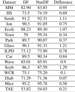
However, quite different results are obtained by compar-ing NeuDF and the DF. Numerical results of comparison of the DF and NeuDF are shown in Table 3. It can be seen from Table 3 that the proposed NeuDF outperforms the DF for all considered data sets. Moreover, the results of com-puting thet statistics for the differences between NeuDF and the DF (see Table 3) are the95%confidence interval
[0.495,0.912]for the mean0.704withp= 0.000003. The t-test demonstrates the clear outperforming of NeuDF in comparison with the DF.
Let us formally compare also the RF and NeuDF as a extreme cases among the considered models models. By computing the t statistics for the differences between
Table 3: Comparison of the NeuDF with DF
Dataset DF NueDF Difference
MM 82.90 83.85 0.95
HS 73.5 74.19 0.69
Seeds 91.2 92.31 1.11
Ion 90.3 91.05 0.75
Ecoli 88.23 89.30 1.07
Yeast 59 59.34 0.34
Park 89.7 90.07 0.37
Glass 90.1 91.31 1.21
ILPD 73.12 73.90 0.78
Car 89.5 90.34 0.84
Wave 85.01 85.91 0.9
Soyb 86.3 87.59 1.29
WCR 75.1 75.20 0.1
Diab 71.29 71.36 0.07
Mice 95.2 95.78 0.58
TAE 53.82 54.03 0.21
NeuDF and the RF, we get the 95% confidence interval
[1.047,2.277]for the mean1.662withp= 0.000038. We see that NeuDF significantly outperforms the RF.
The same can be said about the MNIST and CIFAR datasets. The corresponding numerical results are shown in Table 4. One can see from Table 4 that NeuRF and NeuDF clearly outperform the RF and the DF, respectively.
Another question is how the accuracy measures of
Table 4: Comparison of the RFs and DFs with their modi-fications for MNIST and CIFAR data sets
Dataset RF NeuRF DF NeuDF
MNIST 96.04 96.44 98.4 99.20
Figure 5: Accuracy measures as a function of the decision tree group numbers for the Ecoli dataset.
Figure 6: Accuracy measures as a function of the decision tree group numbers for the MNIST dataset.
Figure 8: Accuracy measures as a function of the hidden layer numbers for the MNIST dataset.
Figure 9: Accuracy measures as a function of the decision tree numbers in every RF for the Ecoli dataset.
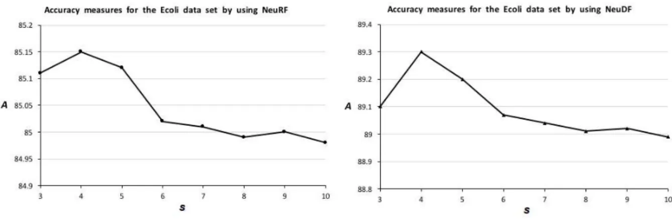
NeuRF and NeuDF depend on the decision tree group num-berss, i.e., on the tuning parameter s. Fig. 5 illustrates these dependences for the Ecoli dataset by using NeuRF (the left plot) and NeuDF (the right plot). It can be seen from the obtained results that there is an optimal values which provides the largest accuracy. This value is4, and it coincides for NeuRF as well as for NeuDF. The same re-sults are obtained for the MNIST dataset (see Fig. 6). It is interesting to note that the optimal values ofscoincide for the Ecoli and MNIST datasets. However, this is just a co-incidence. If we perform the same numerical experiments, for example, with the Yeast dataset, then we get optimal values= 6.
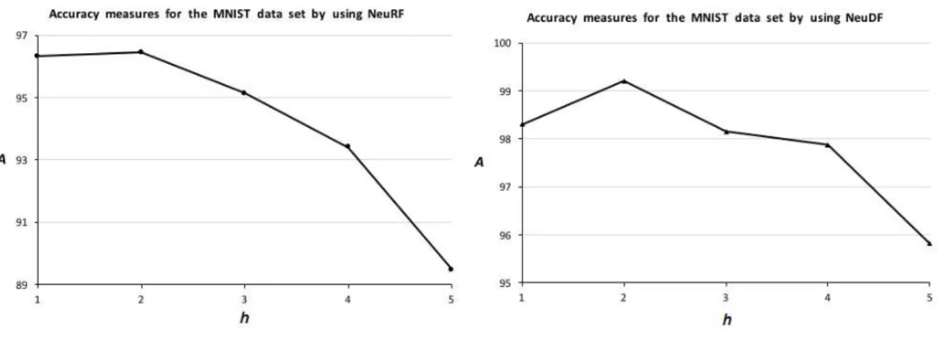
We also investigate how the number of hidden layersh in every neural network impacts on the the accuracy mea-sures. The corresponding curves are shown in Figs. 7-8. Here we again have an optimal value ofh, which provides the largest accuracy. It is interesting to note that the in-crease of the hidden layers does not improve the results. Moreover, this increase makes the results worse. It can be explained by the overfitting effect when a lot of training pa-rameters of the modified RF (weights of trees) are replaced by a lot of connection weights of the neural network. Fi-nally, we investigate how the accuracy measures depend on the numberT of decision trees in every RF. Figs. 9-10 clearly shows that the accuracy measures increase with T, but the computational complexity increases also in this case.
6
Conclusion
New classification models based on combination of the DF and the neural network have been presented in the paper. The main idea underlying these models is to improve RFs and the DF by combining the class probability distributions produced by decision trees for every training example by using a series of identical shallow neural networks with shared weights.
The proposed models have a number of advantages. First of all, we replace a simple rule for the class probability distribution combination (averaging) by a more complex function implemented by the neural network, which aims to minimize a classification loss function. Second, the neural network allows us to simply use various loss func-tions for computing the optimal RF class probability dis-tributions. This leads to opportunity to solve tasks differ-ent from the standard classification, for example, transfer learning. Moreover, by applying the proposed models, we can modify the stacking algorithm used in the DF extending a set of the augmented features by some new functions of the tree class probability vectors. The investigation of new augmented features is a very interesting problem which can be viewed as a direction for further research.
It should be noted that the proposed models have not demonstrated a significant improvement when they were applied to a separate RF. A small increase of the accuracy
measures for many datasets in this case is compensated by additional computations because of the neural network training. However, numerical experiments have illustrated that the proposed combinations may be very effective for the DF because it forms the appropriate augmented features in the stacking algorithm. That is why we have considered modifications of RFs as well as the DF in the paper.
The neural networks in the proposed models are trained by using a training part of datasets. At the same time, a di-rection for further research is to change the neural network learning strategy. For example, they may learn by using testing data or a combination of training and testing data. The above changes may lead to outperforming results.
Acknowledgement
This work is supported by the Russian Science Foundation under grant 18-11-00078.
References
[1] L. Bertinetto, J. Valmadre, J.F. Henriques, A. Vedaldi, and P.H.S. Torr. Fully-convolutional siamese net-works for object tracking. arXiv:1606.09549v2, 14 Sep 2016.
[2] G. Biau and E. Scornet. A random forest guided tour. arXiv:1511.05741v1, Nov 2015.
[3] G. Biau, E. Scornet, and J. Welbl. Neural random forests. arXiv:1604.07143v1, Apr 2016.
[4] L. Breiman. Bagging predictors. Machine Learn-ing, 24(2):123–140, 1996. https://doi.org/ 10.1023/A:1018054314350
[5] L. Breiman. Random forests. Machine learning,
45(1):5–32, 2001. https://doi.org/10.
1023/A:1010933404324
[6] J. Bromley, J.W. Bentz, L. Bottou, I. Guyon, Y. Le-Cun, C. Moore, E. Sackinger, and R. Shah. Signature verification using a siamese time delay neural network. International Jour-nal of Pattern Recognition and Artificial In-telligence, 7(4):737–744, 1993. https: //doi.org/10.1142/S0218001493000339
[7] T. Christensen C. Hettinger, B. Ehlert, J. Humpherys, T. Jarvis, and S. Wade. Forward thinking: Build-ing and trainBuild-ing neural networks one layer at a time. arXiv:1706.02480v1, Jun 2017.
539–546. IEEE, 2005. https://doi.org/10. 1109/CVPR.2005.202
[9] A. Criminisi, J. Shotton, and E. Konukoglu. Deci-sion forests: A unified framework for classification, regression, density estimation, manifold learning and semi-supervised learning.Foundations and Trends in Computer Graphics and Vision, 7(2-3):81–227, 2011.
https://doi.org/10.1561/0600000035
[10] M.E.H. Daho, N. Settouti, M.E.A. Lazouni, and M.E.A. Chikh. Weighted vote for trees aggregation in random forest. In2014 International Conference on Multimedia Computing and Systems (ICMCS), pages 438–443. IEEE, April 2014.https://doi.org/ 10.1109/ICMCS.2014.6911187
[11] R.A. Dara, M.S. Kamel, and N. Wanas. Data depen-dency in multiple classifier systems.Pattern Recog-nition, 42(7):1260 – 1273, 2009. https://doi. org/10.1016/j.patcog.2008.11.035
[12] J. Demsar. Statistical comparisons of classifiers over multiple data sets.Journal of Machine Learning Re-search, 7:1–30, 2006.
[13] K. Fawagreh, M.M. Gaber, and E. Elyan. Ran-dom forests: from early developments to recent ad-vancements. Systems Science & Control Engineer-ing, 2(1):602–609, 2014. https://doi.org/ 10.1080/21642583.2014.956265
[14] A.J. Ferreira and M.A.T. Figueiredo. Boosting algo-rithms: A review of methods, theory, and applica-tions. In C. Zhang and Y. Ma, editors,Ensemble Ma-chine Learning: Methods and Applications, pages 35–85. Springer, New York, 2012.https://doi. org/10.1007/978-1-4419-9326-7\_2
[15] R. Genuer, J.-M. Poggi, C. Tuleau-Malot, and N. Villa-Vialaneix. Random forests for big data.Big Data Research, 9:28–46, 2017. https://doi. org/10.1016/j.bdr.2017.07.003
[16] M. Hibinoa, A. Kimurab, T. Yamashitaa, Y. Ya-mauchia, and H. Fujiyoshi. Denoising random forests. arXiv:1710.11004v1, Oct 2017.
[17] J. Hu, J. Lu, and Y.-P. Tan. Discriminative deep metric learning for face verification in the wild. In The IEEE Conference on Computer Vision and Pattern Recognition (CVPR), pages 1875–1882. IEEE, 2014. https://doi.org/ 10.1109/CVPR.2014.242
[18] Y. Ioannou, D. Robertson, D. Zikic, P. Kontschieder, J. Shotton, M. Brown, and A. Criminisi. Decision forests, convolutional networks and the models in-between. arXiv:1603.01250v1, Mar 2016.
[19] A. Jurek, Y. Bi, S. Wu, and C. Nugent. A sur-vey of commonly used ensemble-based classifica-tion techniques. The Knowledge Engineering Re-view, 29(5):551–581, 2014. https://doi.org/ 10.1017/S0269888913000155
[20] H. Kim, H. Kim, H. Moon, and H. Ahn. A weight-adjusted voting algorithm for ensemble of classifiers. Journal of the Korean Statistical Soci-ety, 40(4):437–449, 2011. https://doi.org/ 10.1016/j.jkss.2011.03.002
[21] P. Kontschieder, M. Fiterau, A. Criminisi, and S.R. Bulo. Deep neural decision forests. In Proceedings of the IEEE International Conference on Computer Vision, pages 1467–1475, 2015. https://doi. org/10.1109/ICCV.2015.172
[22] A. Krizhevsky and G. Hinton. Learning multiple layers of features from tiny images. Technical Re-port 1, Computer Science Department, University of Toronto, 2009.
[23] L.I. Kuncheva.Combining Pattern Classifiers: Meth-ods and Algorithms. Wiley-Interscience, New Jersey, 2004.
[24] Y. LeCun, L. Bottou, Y. Bengio, and P. Haffner. Gradient-based learning applied to document recog-nition. Proceedings of the IEEE, 86(11):2278– 2324, 1998. https://doi.org/10.1109/5. 726791
[25] H. B. Li, W. Wang, H. W. Ding, and J. Dong. Trees weighting random forest method for classifying high-dimensional noisy data. In 2010 IEEE 7th Interna-tional Conference on E-Business Engineering, pages 160–163. IEEE, Nov 2010. https://doi.org/ 10.1109/ICEBE.2010.99
[26] M. Lichman. UCI machine learning repository, 2013.
[27] G. Louppe. Understanding random forests: From the-ory to practice. arXiv:1407.7502v3, June 2015.
[28] D. Maji, A. Santara, S. Ghosh, D. Sheet, and P. Mi-tra. Deep neural network and random forest hy-brid architecture for learning to detect retinal ves-sels in fundus images. In Engineering in Medicine and Biology Society (EMBC), 2015 37th Annual In-ternational Conference of the IEEE, pages 3029– 3032. IEEE, Aug 2015.https://doi.org/10. 1109/EMBC.2015.7319030
[29] K. Miller, C. Hettinger, J. Humpherys, T. Jarvis, and D. Kartchner. Forward thinking: Building deep ran-dom forests. arXiv:1705.07366, 20 May 2017.
New York, 2012.https://doi.org/10.1007/ 978-1-4419-9326-7\_1
[31] Y. Ren, L. Zhang, and P. N. Suganthan. En-semble classification and regression-recent develop-ments, applications and future directions [review article]. IEEE Computational Intelligence Maga-zine, 11(1):41–53, 2016.https://doi.org/10. 1109/MCI.2015.2471235
[32] L. Rokach. Ensemble-based classifiers.Artificial In-telligence Review, 33(1-2):1–39, 2010. https:// doi.org/10.1007/s10462-009-9124-7
[33] L. Rokach. Decision forest: Twenty years of re-search. Information Fusion, 27:111–125, 2016.
https://doi.org/10.1016/j.inffus. 2015.06.005
[34] C.A. Ronao and S.-B. Cho. Random forests with weighted voting for anomalous query access detec-tion in reladetec-tional databases. InArtificial Intelligence and Soft Computing. ICAISC 2015, volume 9120 of
Lecture Notes in Computer Science, pages 36–48, Cham, 2015. Springer. https://doi.org/10. 1007/978-3-319-19369-4\_4
[35] W. Shen, Y. Guo, Y. Wang, K. Zhao, B. Wang, and A. Yuille. Deep regression forests for age estimation. arXiv:1712.07195v1, Dec 2017.
[36] W. Shen, K. Zhao, Y. Guo, and A. Yuille. Label dis-tribution learning forests. arXiv:1702.06086v4, Oct 2017.
[37] L.V. Utkin and M.A. Ryabinin. Discriminative metric learning with deep forest. arXiv:1705.09620v1, May 2017.
[38] L.V. Utkin and M.A. Ryabinin. A deep forest for transductive transfer learning by using a consen-sus measure. In A. Filchenkov, L. Pivovarova, and J. Zizka, editors, Artificial Intelligence and Natu-ral Language. AINL 2017, volume 789 of Communi-cations in Computer and Information Science, pages 194–208. Springer, Cham, 2018. https://doi. org/10.1007/978-3-319-71746-3\_17
[39] L.V. Utkin and M.A. Ryabinin. A Siamese deep forest.Knowledge-Based Systems, 139:13–22, 2018.
https://doi.org/10.1016/j.knosys. 2017.10.006
[40] S. Wang, C. Aggarwal, and H. Liu. Using a ran-dom forest to inspire a neural network and improv-ing on it. In Proceedings of the 2017 SIAM In-ternational Conference on Data Mining, pages 1– 9. Society for Industrial and Applied Mathemat-ics, Jun 2017.https://doi.org/10.1137/1. 9781611974973.1
[41] D.H. Wolpert. Stacked generalization. Neural net-works, 5(2):241–259, 1992. https://doi.org/ 10.1016/S0893-6080(05)80023-1
[42] M. Wozniak, M. Grana, and E. Corchado. A survey of multiple classifier systems as hybrid systems. Infor-mation Fusion, pages 3–17, 2014.https://doi. org/10.1016/j.inffus.2013.04.006
[43] P. Yang, E.H. Yang, B.B. Zhou, and A.Y. Zomaya. A review of ensemble methods in bioinformatics. Cur-rent Bioinformatics, 5(4):296–308, 2010.https:// doi.org/10.2174/157489310794072508
[44] Z.-H. Zhou.Ensemble Methods: Foundations and Al-gorithms. CRC Press, Boca Raton, 2012.
[45] Z.-H. Zhou and J. Feng. Deep forest: To-wards an alternative to deep neural networks. arXiv:1702.08835v2, May 2017.
![Figure 1: The architecture of the cascade forest [45].](https://thumb-us.123doks.com/thumbv2/123dok_us/8036600.2128022/4.892.119.794.121.446/figure-architecture-cascade-forest.webp)