A Global k-means Approach for Autonomous Cluster Initialization of Probabilistic Neural Network

A Global

k

-means Approach for Autonomous Cluster Initialization of

Probabilistic Neural Network

Roy Kwang Yang Chang, Chu Kiong Loo and M.V.C. Rao

Multimedia University, Jalan Ayer Keroh Lama, 75450 Melaka, Malaysia E-mail: [email protected]

Keywords: probabilistic neural network, global k-means, condition monitoring

Received: May 14, 2007

This paper focuses on the statistical based Probabilistic Neural Network (PNN) for pattern classification problems with Expectation – Maximization (EM) chosen as the training algorithm. This brings about the problem of random initialization, which means, the user has to predefine the number of clusters through trial and error. Global k-means is used to solve this and to provide a deterministic number of clusters using a selection criterion. On top of that, Fast Global k-means was tested as a substitute for Global k-means, to reduce the computational time taken. Tests were done on both homescedastic and heteroscedastic PNNs using benchmark medical datasets and also vibration data obtained from a U.S. Navy CH-46E helicopter aft gearbox (Westland).

Povzetek: Opisana je metoda nevronskih mrež.

1

Introduction

The proposed model in this paper uses PNN as our choice of neural network for pattern classification problems. The Probabilistic Neural Network was first introduced in 1990 by Specht [1] and puts the statistical kernel estimator [2] into the framework of radial basis function networks. [3] We then used EM to train the PNN for the simple fact that it can help reduce the number of neurons that were committed in the network. The proposed model can be used in the field of condition monitoring which is garnering more attention due to its perks of time and cost savings. That is the reason why more focus should be spent on the creation of a more error tolerant and accurate yet fast diagnostic model.

The EM method used as the training algorithm for the network has its advantages and disadvantages. In general it is hard to initialize and the quality of the final solution depends heavily on the quality of the initial solution. [4] Initialization of the number of clusters needed has to be done randomly by the user in a series of trial and error values. This brings about an unwanted stochastic nature in the model. Therefore, in order to build an autonomous and deterministic neural network, we opted to use Global k-means to help automatically find the optimum number of clusters based on minimizing the clustering error.

In section 2, the PNN model is briefly discussed followed by section 3 where the E-step and the M-step of the EM method is showed together with the flaws of EM. Section 4 details cluster initialization with a brief discussion on two methods of cluster determination, which is Global k-means and its variant, Fast Global k -means. Experiments on Westland and benchmark medical datasets were done in section 5 to compare

results between Global k-means and random initialization together with Global k-means and Fast Global k-means. Section 6 will conclude the paper.

2

Probabilistic neural network

Probabilistic Neural Network was introduced by Donald Specht in a series of two papers, namely “Probabilistic Neural Networks for Classification, Mapping or Associative Memory” in 1988 [5] and “Probabilistic Neural Networks” in 1990 [1]. This statistical based neural network uses Bayes theory and Parzen Estimators to solve pattern classification problems. The basic idea behind Bayes theory is that it will make use of relative likelihood of events and also a priori information, which in our case would be inter-class mixing coefficients. As for Parzen Estimators, it is a classical probability density function estimator.

Let us assume the dataset, X, will be partitioned into

K number of subsets where

X

=

X

₁

∪

X

₂

∪

...

∪

X

_K and each subset having Nk number of sample size, it

would also mean

∑

K_k=1

N

_k

=

N

where N is the size of our sample. This four-layer, feed forward, supervised learning neural network reserves the lowest layer as input neurons and accepts d-dimensional input vectors. Each dimension of the input vector is passed to its corresponding input neuron.

)

2

(

exp

)

2

(

1

)

(

₂ , 2 , 2 2 , , k m k m d k m k m

X

X

σ

υ

σ

ρ

−

−

Π

=

(1)

and this specifies the GBF for m-th cluster in the k-th class where

σ

_m2_,k is the variance,

υ

_m,k is the cluster centroid and d represents the dimension of the input vector.

The third layer of the PNN is where the class conditional probability density function is estimated, given by the formula

∑

=

=

Mk

m mk mk

k

X

X

f

(

)

₁

β

_,

ρ

_,

(

)

(2)

where

M

_k is the number of clusters for class k and

k m,

β

is the intra-class mixing coefficient that can be defined as below.

∑

=

=

k

M

m1

β

m,k

1

(3)

The PNN model has a fourth layer which is used as a decision layer to choose the class with the highest probability. An inter-class mixing coefficient,

α

_k, will be used to increase the accuracy of the result.

α

_k is obtained by the inverse of its sample size, Nk . Therefore

the summation of all

α

_k shall be bound to 1.

ο

_k depicts the probability of the input vector being class k.

)

(

x

f

_k k

k

α

ο

=

(4)

)

max

arg(

1 k K k

decision

ο

≤ ≤

=

(5)

The advantage that PNN has is that it interprets the network’s structure in probability density functions due to its statistical nature. On the downside, the number of nodes that is committed in the PNN can be extremely huge if the training dataset is large. This is because one neuron is created for each training pattern. This makes the PNN simply infeasible for large datasets. Therefore another training method that does not commit every training pattern as a node in the neural network should be used. And for this purpose, we have selected the Expectation-Maximization (EM) method.

3

Learning algorithm

In the learning algorithm, two parameters of the model are adjusted to obtain better results in classification. In each E-step and M-step, the mean and the variance parameter is constantly tweaked until the log posterior likelihood function shows minimal difference.

To calculate the new mean and variance values, EM deploys a weight parameter which is also adjusted after each step.

3.1

Expectation-Maximization

Expectation-Maximization (EM) [6] by Dempster et. al. in 1977 is a powerful iterative procedure which converges to an ML estimate. Basically the EM method consists of two steps, namely the E-step and the M-step. Both steps will be iterated until the change in the log posterior likelihood function is minimal.

)

(

log

log

1

f

X

L

K

k k

f

=

∑

= (6)

In the E-step, the missing or hidden data is estimated given the observed data and the current parameter estimate. It will use the PDF estimated in the second layer of the PNN as defined in Equation 1 together with intra-class mixing coefficient to estimate the weight parameter.

∑

=

=

k

M

i ik ik

k m k m k m

X

X

W

1 , ,

, , ,

)

(

)

(

ρ

β

ρ

β

(7)

Next comes the M-step that uses the data estimated in the E-step, the weight parameter,

W

_m,k, to form a likelihood function and determine the ML estimate of the parameter. It calculates the new values of the cluster centroid,

υ

_m,k, the variance,

σ

_m2_,k, and the intra-class

mixing coefficients,

β

_m,k, using the weight calculated from the E-step. The equations for the parameter updates are given as below.

∑

∑

= =

=

k k N

n mk

N

n mk

k m

X

W

X

X

W

1 , 1 , ,

)

(

)

(

υ

(8)

)

(

)

(

1 , 1 2 , , 2 ,

X

W

d

X

X

W

k k N

n mk

N

n mk mk

k m

∑

∑

= =

−

=

υ

σ

(9)

∑

=

=

Nk

n mk

k k

m

W

X

N

1 ,

,

(

)

1

β

(10)

requires initialization in the form of, number of clusters to be expected of the neural network. The initialization quality severely affects the final outcome of the network. In order to aid in this matter, a method called Global k -means will be chosen as a precursor to find out how many clusters are needed for a certain dataset before being fed into the PNN with EM for training.

4

Cluster initialization

Part of the problems faced by the model is determining the number of clusters needed prior to learning. This is usually inputted by the user through a series of trial and error values. Also the usage of random initialization does not provide deterministic results. Global k-means and Fast Global k-means can overcome these problems.

4.1

Global

k

-means

Introduced by A. Likas, N. Vlasis and J.J. Verbeek in the paper entitled “The Global k-means clustering algorithm” in 2003, the concept of clustering with Global

k-means is partitioning the given dataset into M clusters so that a clustering criterion is optimized. The common clustering criterion is the sum of squared Euclidean distances between each data point and the cluster centroid.

∑

∑

= =

−

=

k Mk

m i m

N i

k

X

M

M

E

1

2 1

1

,...,

)

(

υ

(11)

Global k-means deploys the k-means algorithm to find locally optimal solutions by trying to keep the clustering error to a minimum. The k-means algorithm starts by placing the cluster center arbitrarily and at each step moves the cluster center with the aim to minimize the clustering error. The down side to this algorithm is that it is sensitive to the initial position of the cluster centers. To overcome this, k-means can be scheduled to run several times and each time with a different starting point. The gist of Global k-means is that instead of trying to find all cluster centers at once, it proceeds in an incremental fashion. Incremental in the sense that one cluster center is found at a time.

Assume a K-clustering problem is to be solved; the algorithm starts by solving for a 1-clustering problem and the placement of the cluster center in this instance would equal the centroid of the given dataset. The next step would be to add another cluster center at its optimal position, given, the first cluster center has already been found. To do this, N-executions of k-means algorithm will be executed with the initial positions of the cluster centers being the first cluster which was found when solving for a 1-clustering problem and the second cluster’s starting position will be at

x

_n where

.

1

≤

n

≤

N

The final answer for a 2-clustering problem will be the best solution from the N-executions of k -means algorithm. Let (c1(k),…,ck(k)) denote the final

solution for the k-clustering problem. We will solve it iteratively which means solving a 1-clustering problem,

then a 2-clustering problem, until a (k-1)-clustering problem and the solution of k-clustering problem can be solved by performing N-executions of k-means algorithm with starting positions of (c1(k-1),…,c(k-1)(k-1),Xn). A

simple pseudo code of it will be

Problem: to solve k-clustering problem for dataset, X

For i=1 to k

{

If i = 1 then

c

_i

=

centroid of dataset, X

Else

For j=1 to N

Run k-means with initial values of {

c

_i

,...,

c

_i−1

,

X

_j}

}

With the final solution, (c1(k),…,ck(k)), Global k

-means has actually found solutions of all k-cluster problem where k=1,…,K without needing any further computations. This assumption seems very natural: we expect that the solution of a k-clustering problem to be reachable (through local search) from the solution of a (k-1)-clustering problem, once the additional center is placed at an appropriate position within the data set. [10] Alas, the downside is that the computational time of Global k-means can be rather long.

4.2

Fast Global

k

-means

Using this method will help reduce the computational time taken by the Global k-means algorithm. The core difference is that, Fast Global k -means does not perform N-executions of k-means algorithm with starting positions of (c1(k-1),…,c(k-1)

(k-1),Xn). Instead, what the algorithm does is to calculate the

upper bound

E

_n

≤

E

−

b

_n on the resulting error, En, for

every instances of Xn. We define E as the error value of

(k-1)-clustering problem and bn as

∑

= −

−

−

=

N_j j _{n j}

k

n

d

x

x

b

₁

max(

₁ 2

,

0

)

(12)

with

d

_kj₋₁ as the squared Euclidean distance between xj and the cluster centroid which it belongs to.

After obtaining the value of bn, select the xi that

maximizes bn and make it the new cluster centroid that

will be added. This is because by maximizing the value of bn, we are at the same time minimizing the En value

which as stated is our error. The new cluster centroid, xn,

will allocate all data points which have a smaller squared Euclidean distance from xn rather than from their

previous cluster centroid

d

_kj₋₁. In view of that, the reduced clustering error for all those reassigned data points is j_{1 n j} 2

k x x

Since the k-means algorithm is guaranteed to decrease the clustering error at each step,

E

−

b

_nupper bounds the error measure that will be obtained if we run the algorithm until convergence after inserting the new center at xn (this is the error measure used in the Global

k-means algorithm). [10]

5

Experiments and results

5.1

General description

First, a test is conducted using EM-based PNN with two types of initialization, random and Global k-means. The benchmark medical datasets together with the Iris dataset was used for this purpose. Then, a test between EM-based PNN with initialization from Global k-means and Fast Global k-means was done to observe the computational time and also the difference in classification performance. The benchmark medical datasets were used. Next were tests done on Westland vibration dataset using EM-based PNN with Global k -means and also tests between Global k-means and Fast Global k-means to observe its accuracy and computational time.

5.2

Comparative tests between random

initialization and Global

k

-means

Tests on the benchmark medical datasets and the Iris dataset [11] were conducted to observe the effects of random initialization and using Global k-means to initialize the parameter values in EM. The medical datasets consist of data from Cancer, Dermatology, Hepato, Heart and Pima.

The Iris dataset consists of 150 samples and 4 input features. It was tested on PNN trained by EM with randomly initialized cluster centroids and EM with Global k-means initialization. Both the methods were executed in heteroscedastic PNN and in homoscedastic PNN. A ten-fold validation was used. The Iris dataset was set as a 10-clustering problem for Global k-means and the number of cluster centroids returned was based on minimizing the squared Euclidean distance between each data point in a cluster and its centroid. This was then used to set the cluster parameter for random initialization to help it get a better result and assume under similar conditions as the Global k-means.

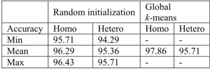
The mean accuracy of the homoscedastic with random initialization is 96.29% whilst the heteroscedastic version reports 95.36% accuracy. But in both cases, they were outdone by the accuracy of EM with Global k-means initialization, whose mean accuracy was 97.86% and 95.71% respectively, for homoscedastic and heteroscedastic PNN. Although random initialization was fed with the number of clusters needed by Global k -means, Global k-means still had the better classification rate.

Table 1: Correct classification rates for the Iris dataset.

Random initialization Global _k-means

Accuracy Homo Hetero Homo Hetero

Min 95.71 94.29 - -

Mean 96.29 95.36 97.86 95.71

Max 96.43 95.71 - -

The Cancer dataset contains 569 samples with a 30 dimension size, whilst the Dermatology dataset contains 358 samples with a 34 dimension size and the Hepato dataset contains 536 samples with a 9 dimension size. The Heart dataset contains 270 samples with a 13 dimension size and two output labels, which are “0” for absence of heart disease and “1” for presence of heart disease. Pima data set is available from machines learning database at UCI [12]. The Pima dataset contains 768 samples with an eight dimension size and has two classes which are diabetes positive and diabetes negative. A ten-fold validation was employed. When running using all the above datasets, Global k-means was set with a higher than required clustering problem to solve and in every case it returns a lower number of clusters which is optimum to the clustering criterion. This was also fed into EM for random initialization.

Table 2: Correct classification rates for the medical datasets by using homoscedastic PNN.

Random initialization Global _k-means Dataset

Min Mean Max Mean Cancer 90.00 90.63 90.96 91.92 Dermatology 60.76 64.28 65.50 69.31 Hepato 37.35 38.51 39.18 39.39 Heart 62.40 63.52 64.40 58.80 Pima 70.29 71.07 71.43 71.29

Table 3: Correct classification rates for the medical datasets by using heteroscedastic PNN.

Random initialization Global _k-means Dataset

Min Mean Max Mean Cancer 94.23 94.52 94.62 95.38 Dermatology 86.87 88.05 89.08 89.54 Hepato 51.22 52.47 53.27 58.57 Heart 75.60 78.00 78.80 82.80 Pima 66.86 68.17 68.86 69.00

the EM with random initialization is not higher than the mean of EM with initialization from Global k-means.

5.3

Comparative tests between Global

k

-means and Fast Global

k

-means

In order to minimize computational time without sacrificing the classification performance, we opted for the Fast Global k-means implementation. Below is a comparison between Global k-means and Fast Global k -means using both heteroscedastic and homoscedastic PNNs which were trained by the EM method. Tests were conducted on the medical datasets using a ten-fold validation and as usual, Global k-means was set to solve a higher clustering problem than required.

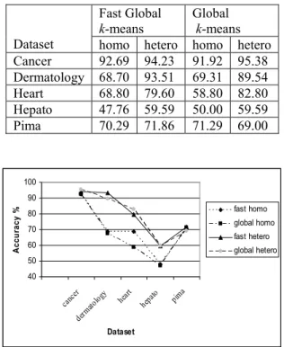
Table 4: Comparison of correct classification rates. Fast Global

k-means Global k-means Dataset homo hetero homo hetero Cancer 92.69 94.23 91.92 95.38 Dermatology 68.70 93.51 69.31 89.54 Heart 68.80 79.60 58.80 82.80 Hepato 47.76 59.59 50.00 59.59 Pima 70.29 71.86 71.29 69.00

40 50 60 70 80 90 100

cancer derma

tolog y

heart _hepato pima

Dataset

A

ccu

racy %

fast homo global homo fast hetero global hetero

Figure 1: Comparison of correct classification rates.

Table 5: Comparison of computational times in seconds. Fast Global

k-means Global k-means Dataset

homo hetero homo hetero Cancer 5.80 14.83 563.20 622.95 Dermatology 11.69 20.95 849.34 950.77 Heart 2.03 5.69 71.08 93.00 Hepato 3.97 4.05 153.88 148.14 Pima 29.55 43.47 3299.11 3427.41

As shown in the results of Table 4 and Figure 1, Fast Global k-means provides a comparable correct classification rate on the benchmark medical datasets. On top of that, it still manages to accomplish its purpose which was to cut down on computational time. And Table 5 clearly supports this matter.

5.4

Westland Vibration Dataset

A real world case study was done; to test the EM trained PNN with initialization parameters obtained from the execution of Global k-means, using the popular benchmark dataset Westland [13]. This dataset consists of vibration time-series data which is gathered from an aft main power transmission of a U.S. Navy CH-46E helicopter by placing eight accelerometers at the known fault sensitive locations of the helicopter gearbox. The data was recorded for various faults including a no-defect case.

Table 6: Westland helicopter gearbox data description. Fault

type Description

2 Plenetary Bearing Corrosion 3 Input Pinion Bearing Corrosion 4 Spiral Bevel Input Pinion Spalling 5 Helical Input Pinion Chipping 6 Helical Idler Gear Crack Propagation 7 Collector Gear Crack Propagation 8 Quill Shaft Crack Propagation 9 No Defect

This dataset consists of 9 torque levels but for our experiment purposes, only the 100% torque level on sensors 1 to 4 is used. As the number of features from this dataset is quite substantial, feature reduction was needed. Wavelet packet feature extraction [14] was used to reduce the dimension of the input vectors without sacrificing too much of the classification performance.

Wavelet packets, a generalization of wavelet bases, are alternative bases that are formed by taking linear combinations of the usual wavelet functions. [15][16] These bases inherit properties such as orthonormality and time-frequency localization from their corresponding wavelet functions. [14] Wavelet packet functions can be defined as

)

2

(

2

)

(

/2

,

t

W

t

k

W

n j n j

k

j

=

−

(13)

where n is the modulation or oscillation parameter, j is the index scale and k is the translation.

For a function, f, the wavelet packet coefficients can be calculated as below

∫

=

=

f

W

f

t

W

t

dt

w

n

k j n

k j k

n

j,,

,

,

(

)

,

(

)

(14)

In brief, the steps are; firstly, decompose the vibration signal using Wavelet Packet Transform (WPT) to extract out the time-frequency-dependant information. For each vibration signal segment, full decomposition is done up to the seventh level. This will produce a group of

2

2

r+1

₋

_{sets of coefficients where r is the resolution}

254 sets of coefficients where each set corresponds to a wavelet packet node. For the coefficients of every wavelet packet node, the wavelet packet node energy ,

n j

e

_, , is computed and this acts as the extracted feature.

∑

=

k k n j n

j

w

e

2

, ,

, (15)

After that, apply a statistical based feature selection criterion to help identify the features that provide the most discrimination amongst the classes of the dataset in focus, Westland. The Fisher’s criterion was used. [17] As a result, the number of features for Westland was reduced to eight and this modified dataset was fed into our model to test for classification rate by usage of Global k-means.

Table 7: Correct classification rates for Westland using homoscedastic and heteroscedastic PNNs.

Accuracy Sensor _{Hetero Homo} 1 96.06 86.06 2 94.51 88.45 3 95.92 87.89 4 95.21 91.41

The performance obtained by the proposed system on the 8-feature, 776-sample Westland dataset strengthens the positive performance that was marked in testing done on benchmark medical datasets.

We then performed further testing on the Westland dataset using Global k-means and its variant, Fast Global

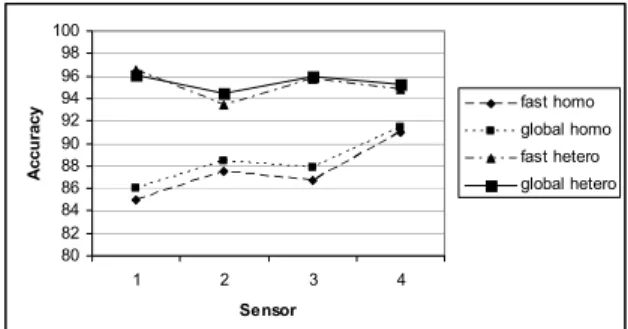
k-means. It was tested on both homoscedastic and heteroscedastic PNNs and again ten-fold validation was applied. As can be seen in Figure 2, the performance in terms of accuracy is comparable between the two methods. Not much accuracy degradation is shown by Fast Global k-means on the Westland sensor 1 to 4 data. Though comparable in terms of accuracy, the time taken by both methods is very different. Global k-means is a far slower method in comparison to the computational time of Fast Global k-means. This justifies our proposal of using Fast Global k-means with our model because though admittedly classification performance degrades, but it is by an acceptable margin and the time reduction is significant.

Table 8: Comparison of correct classification rates for Westland dataset.

Fast Global

k-means

Global

k-means Sensor

homo hetero homo hetero 1 84.93 96.48 86.06 96.06 2 87.46 93.38 88.45 94.51 3 86.76 95.77 87.89 95.92 4 90.99 94.79 91.41 95.21

80 82 84 86 88 90 92 94 96 98 100

1 2 3 4

Sensor

Ac

cu

ra

cy fast homo_{global homo}

fast hetero global hetero

Figure 2: Comparison of correct classification rates.

Table 9: Comparison of computational times in seconds. Fast Global

k-means

Global

k-means Sensor

homo hetero homo hetero 1 6.38 7.99 237.30 234.41 2 5.84 6.63 228.89 226.28 3 5.97 8.42 230.64 234.51 4 6.27 7.55 236.02 229.42

6

Conclusion

References

[1] Specht, D.F.: Probabilistic Neural Network. Neural Networks 3 (1990) 109-118.

[2] E. Parzen.: On the estimation of a probability density function. Annals of Mathematical Statistics 3 (1962) 1065-1076.

[3] Berthold, M.R., Diamond, J.: Constructive Training of Probabilistic Neural Networks. Neurocomputing 19 (1998) 167-183.

[4] Ordonez, C., Omiecinski, E.: FREM: Fast and Robust EM Clustering for Large Data Sets. CIKM (2002).

[5] Specht, D.F.: Probabilistic neural network for classification, mapping, or associative memory. Proceedings of the IEEE International Conference on Neural Networks 1 (1998) 525-532.

[6] Dempster, A.P., Laird, N.M., Rubin, D.B.: Maximum likelihood for incomplete data via the EM algorithm. Journal of the Royal Statistical Society (B) 39 (1977) 1-38.

[7] Wu, C.: On the Convergence Properties of the EM Algorithm. Annals Statistics 11 (1983) 95-103. [8] Xu, L., Jordan, M.I.: On Convergence Properties of

the EM Algorithm for Gaussian Mixtures. Neural Computation 8 (1996) 129-151.

[9] Yang, Z.R., Chen, S.: Robust Maximum Likelihood Training of Heteroscedastic Probabilistic Neural Networks. Neural Networks 11 (1998) 739-747. [10] Likas, A., Vlassis, N., Verbeek, J.J.: The Global k

-means Clustering Algorithm. Pattern Recognition 36 (2003) 451-461.

[11] C. L. Blake, C. J. Merz: UCI Repository of Machine Learning Databases, University of California, Irvine, Department of Information and Computer Sciences (1998).

[12] F. Zarndt: A Comprehensive Case Study: An Examination of Machine Learning and Connectionist Algorithms, MSc Thesis. Dept. of Computer Science, Brigham Young University (1995).

[13] B. G. Cameron: Final Report on CH-46 Aft Transmission Seeded Fault Testing, Westland Helicopters, Ltd., U.K., Res. Paper RP907,1993. [14] Yen, G.G., Lin, K.C.: Wavelet packet feature

extraction for vibration monitoring. IEEE Transactions on Industrial Electronics 47 No. 3 (2000).

[15] Coifman, R.R., Wickerhauser, M.V.: Entropy based algorithms for best basis selection. IEEE Transactions on Information Theory 38 (1992) 713-718.

[16] Wickerhauser, M.V.: Adapted wavelet analysis from theory to software. Natick, MA: Wellesley (1994).