A general accounting framework for ecological systems: a functional taxonomy for connectivist ecology

(1)

THEORETICAL POPULATION tllOLOG\ 40. 78-104 ( 1991 I

A General Accounting Framework for

Ecological Systems: A Functional

Taxonomy for Connectivist Ecology

BRUCE HANNON

Deparrmenr qf Geograph) und Illrnors Narurul H~stoq, Suroey, Unicersir.v of Illinors. l:rhana, Illmois 61801

AND

ROBERT COSTANZA AND ROBERT ULANOWICZ

Chesapeake Biological Laborator?; Center .for Enwonmenral and Esruarine Studies, Universq qf Maryland,

Solomons. Maryland 20688-0038

Received February 1. 1990

Accountmg of material and energy flows has long been an Important tool m ecosystem ecology. But each material is usually handled separately and independently. The connections between materials, energy, plants, animals, etc. have not been incorporated into the accounting framework, and “service” or mforrnation flows (such as flower pollination by bees) are usually ignored. We develop a general accountmg framework that addresses thus deficrency. In our framework, each connection (both physical and informattonal) can be unambiguously asstgned, quantitied, and qualified, and an input-output balance IS easily checked and maintained for each product. Costly independent data collections can be integrated into this common framework to amplify their original usefulness and provide the investigator or ecosystem manager wrth enhanced understanding of the enttre ecosystem from whtch they were taken. The integrated data also allow various ecosystem models to be constructed efficiently, without unnecessary and costly duplication of effort. We present detatled guidehnes for construction of such a framework, followed by examples and applicattons. ‘C 1991 Academic PWSS. IK

Contents

1. Inrroductton. A. What is an accounting system? B. Why use an accounting system?

II. Deoelopment of issues for accounting sysrems m ecology.

III. A general accountrng framework. A. Desiderata. B. The art of choosing stocks and flows. C. Quanttfying the flows. D. Examples. E. Data quality control. IV. Lfses of the general uccounrmg system A. Network analysts and energy

intenstties. B. Simulation modeling. C. Optimization, V Summary and Conclusrons.

0040-5809/91 $3.00

C opynghf ,is 1991 by Academic Press. Ins All rights of reproductmn I” any lorm reserved

(2)

ACCOUNTING FOR ECOLOGICAL SYSTEMS 79

I. INTRODUCTION

A. What Is an Accounting System?

In biology, species are identified and classified according to a general system first devised by Linnaeus. The assignment of any particular species to a place in the hierarchic system is based on genetic and morphological similarities between organisms. Classifications are often debated and reassignments are occasionally made, but progress in biology without such a system would not be possible.

In ecology, although functional connections between the many species and their environment have been observed for decades, there is no accepted general accounting system for noting and comparing these connections. We propose a functional taxonomy for quantitative ecology-a general ecological accounting system. It is a framework in which the quantified connections between organisms (individual species, collections of species) and their abiotic environment can be placed and balanced, without ambiguity, omission, or double counting exchanges, at any scale which an investigator chooses. By connections we mean any kind of exchange of product (e.g., nectar from a plant, pollination time from an insect) between ecological processes (e.g., insect and plant). A connectivist ecology is one in which the choice of process definition is largely discretionary, but once the choice is made, the interconnection flows are determined and are of primary importance in the ensuring system description. This is in contrast to the Linnaean taxonomy, in which the place of an organism in the system is determined by its structure and evolutionary history, and flows between it and the rest of the system are of secondary importance at best.

This general ecological accounting system is the product of years of debate among ecological modelers, and it also benefits from years of debate and experience gained in national economic accounting.

B. Why Use an Accounting System?

The principal advantage of a universal accounting system in ecology is that it allows the material, energy, and service flows between all the parts of an ecosystem to be systematically placed in a common framework. Ecologists have long been involved in material and energy flow accounting (Hannon, 1973; Finn, 1976), but in the past each type of material (e.g., nitrogen) or energy was accounted for independently of all the rest. To qualify as ecosystem accounting, the interconnections between all the material and energy (and service) flows must also be included. This is the purpose of the framework proposed below.

(3)

80 HANNON, COSTANZA. AND L’LANOWICZ

extant data bases (gathered for unrelated purposes) in that they can be incorporated and commensurately scaled into the same framework as current data. Together, old and new data can reside in a framework that provides the format for evaluation of whole ecosystem function (e.g.. Hannon and Joiris, 1989).

In more detail, the use of an ecological accountmg system could therefore assure ecosystem analysts and managers that a research effort on a particular ecosystem was done: 1. with full awareness of the system boundary (in space and time); 2. such that balance of materials, energy, and service flows for each compartment of the ecosystem under study was achieved; 3. with quantified connection to the rest of that ecosystem of any particular species of special interest; 4. in a way that allowed the compila- tion of data from various researchers of differing interests into a framework of growing utility.

The first known accounting framework for physical systems was developed in the 18th century by Turgot and Quesnay. The first large system accounting framework in which quantified interconnecting flows were measured was in the field of economics. Kuznets (1946) defined the concept of net output of an economy (Gross National Product) as a way of quantitatively comparing the activity levels of the economies of various countries. Leontieff (1941) defined a matrix structure for collecting the flows between various producing sectors so that he could determine the total output required to produce a unit of net output of each sector of the whole economy. This procedure is of crucial importance in planned economies and was of great use to the U.S. government just prior to and during World War II. Many countries (especially Japan) use the Leontieff system to look for production “bottlenecks” and to plan the development of their economies in specified areas. Stone (1963) refined the Leontieff approach to allow unambiguous accounting of multiple inputs and outputs.

With Stone’s contribution, the economic accounting procedure concept was

essentially complete. The use of such accounting systems for public policy (Koopmans, 195 1) and their theoretical implications for ecology (Amir. 1979) have been reported.

We have been guided in our development of an ecological accounting

(4)

II. DEVELOPMENTOF ISSUES INVOLVING ACCOUNTING SYSTEMS IN ECOLOGY

Quantifying a population’s food sources and losses in terms of biomass and numbers can lead to useful insights. However, when the interaction of living organisms with their non-living surroundings are measured, it is only natural to seek a physical yardstick. The fact that a significant portion of an organisms’ surroundings consists of other living populations leads us to seek consistency by applying the same physical yardstick to interbiotic transfers.

Lindeman (1942) first constructed a budget of the flows connecting the biotic and non-living components of a senescent Michigan lake ecosystem. Lindeman’s work is considered by many to be the prototype of modern ecosystems accounting schemes. It emphasized the relational or connectivist view of ecology. Not only is a population related to its physical

surroundings, but it is connected in the same terms to other populations.

Through Lindeman, ecology experienced a hierarchical leap from the study

of populations to a consideration of the wider scope and scale of ecosystems.

Also important were the units in which Lindeman’s accounting ultimately were reported-those of energy. Energy is a physical charac- teristic and can be used to express the physical nature of a biological

system in a way that is non-reducfionistic. Furthermore, energy is a con-

struct that derives from the phenomenological science of thermodynamics. By accounting for all energy entering and leaving each population, one is

recapitulating the first law of thermodynamics-that energy is neither

created nor destroyed. But the first law begs the invocation of the second, which says (in one of its myriad of equivalent forms) that useful output from any process cannot occur without the degradation of some of the process input into less useful forms. The inviolability of the second law impresses a pyramidal form upon any discernible trophic chain of energetic transfers. The amounts of energy available to be passed on to higher trophic links must become progressively smaller.

(5)

82 HANNON. C‘OSTANZA. AND ULANOWICZ

The shift towards whole system budgets afforded other connectivist insights. Connecting elements together in an overall budget made rt possible to trace indirect causes in quantitative terms. However, the number and complexity of such indirect linkages easily overwhelms one’s perceptual capacities. So to make any progress in evaluating indirect effects one must resort to systematic analytical techniques. Of course, the question of indirect effects is hardly limited to ecology. It is a significant issue in economics as well. It was an economist (Leontieff, 1941) who first success- fully applied the techniques of matrix algebra to the task of accounting for indirect effects. Some economists (Daly, 1968) have suggested that ecological flows be included in the Leontieff approach.

Hannon (1973) demonstrated how Leontieffs methods could be applied to ecological budgets. There followed copious efforts to apply “input-output” analysis to various ecosystems and to modify the analytical techniques to address better various issues of ecological concern. Patten et al. (1976) combined input-output analysis with general systems theory to extend the notion of an ecological niche to include indirect impacts and effects. Barber (1978) emphasized the probabilistic nature of ecological transfers and spotlighted the Markovian assumptions underlying the Leontieff approach. Finn (1976) studied the indirect effects that many system components exert upon themselves and showed how to estimate the fraction of the total system activity that is devoted to recycle.

Amir (1979) laid out the economist’s views on equilibrium in ecological systems, including the interpretations of value, cost, and price. Ulanowicz and Kemp (1979) remarked how the algebraic powers of the matrix of nor- malized transfers (the technical coefftcients of economics) provide information on how much medium traverses trophic pathways of various lengths. They used the successive matrix powers to transform arbitrary webs of trophic interactions into Lindeman-like chains or pyramids of flows.

Matis and Patten (1981) attempted to incorporate the contents, or stocks, associated with the system components into the analysis of indirect effects and sketched out what they called “environ analysis.” Unlike the standard input-output analysis of systems that must balance around each component, environ analysis treats systems that are unbalanced and change via an assumed set of linear dynamics. Hannon (1986) examined the stability of such linear systems and evaluated several control strategies (either endogenous or externally applied) that could guide the system towards particular configurations.

(6)

pollination). Implicit in single medium analyses are the assumptions that all inputs to a compartment have equal effect upon the recipient population, and that only one product issues from each compartment (usually its biomass as food to predators.) The latter assumption is not valid because organisms produce by-products such as feces, urine, detritus, and other exudates. How does one treat these multiple products that issue from a population or process? But perhaps even more problematic is the likelihood that the various foods consumed by each predator differ in their utilities to the consumer. How do we weight the various inputs to a compartment to reflect their relative utilities? Fortunately, one solution to both these difficulties is suggested by recent work in input-output theory.

In economics, one view of the origin of prices is that they account for the cumulative value added to a particular item at every step in the economic process from raw materials to finished product.’ In ecology it is sometimes possible to make analogous calculations (Costanza and Neill, 1984). If a system has only one external input of a type not produced in the system, it is then possible to trace back through the network to identify the amounts of that input medium that were necessary to create any given connection. That is, one can estimate the portion of the input that has been “embodied” into each connection. It has been shown (Costanza, 1980; Costanza and Herendeen, 1984) how all the energies contributing to various economic products are correlated to their market prices. In the special case of a network with but a single medium (e.g., all energy flows), a particular transfer between higher trophic levels may yield value when directly measured (a certain number of calories). However, the de facto value of the flow in a systems context would reflect more the amount of the external input (e.g., sunlight) that went into creating the given flow. The ratio of the latter quantity to the former is called an “intensity” and can be used to weight the various inputs to a population so as to allow a legitimate comparison among these inputs.

Similarly, intensities can be calculated for an ecosystem description which has multiple outputs as well as multiple inputs. That procedure is more complex (Costanza and Hannon, 1989) and requires the accounting system described below.

Amir (1987) has discussed the use of an ecological accounting system, both static and dynamic, to elaborate on the formal connections between ecology, thermodynamics, and economics. He points out that the “intensities” of which we speak are measured in terms of an external input and that we therefore must choose which external input should form the basis of the intensities. In the development of the general accounting system,

(7)

84 HANNON, COSTANZA. AND ULANOWICZ

however. we are not proposing the use of intensities or any other kind of

model. We view the accounting system as a necessary underpinning for any kind of ecosystem model which claims to be consistent with any other kind. The accounting system which we propose forms the basis for consistent comparison of model results. Amir points out that these intensities are reminiscent of economic prices which arise from ecological resource allocation problems, just as they do in economics.

III. A GENERAL ACCOUNTING FRAMEWORK

A. Desiderata

We can now set forth, in general terms, the minimum desired criteria for an accounting framework capable of handling both ecological and economic systems. These can be summarized as (1) generality; (2) comprehensiveness; (3) uniqueness; and (4) quality control. These are described in more detail below.

Generalit)?

The accounting framework should exhibit a high degree of universality or generality, in the sense that its usefulness should not be limited to any particular system or temporal or spatial scale. It should be applicable to both ecological and economic systems, on spatial and temporal scales ranging from microcosms to the planet as a whole. We desire this charac- teristic so as to begin to make valid comparisons between divergent systems and to start to bridge the wide chasm that currently exists between ecology and economics. We wish to be able to combine data from different geographic regions of the same ecosystem into the same framework, for a given time period.

Comprehensiveness

(8)

Uniqueness

The accounting framework should provide a unique and unambiguous place for each measurable type of connection. The physical or thermo- dynamic quality of the connection must be recognized and treated con- sistently and the system boundaries should be physically definable in a discoverable way.

Quality control

The accounting framework should exhibit an ability to deal with information of varying quality in a simple and consistent way. The precision of the data for each connection should carry its own mark of reliability and the change in that mark should be specified as the data are mingled arithmetically with other data.

B. The Art of Choosing Stocks and Flows

When asked to list the important components of the system, it is extremely rare that two investigators will spontaneously enumerate the same elements. Of course, the subjective biases that determine what is actually measured will color the ensuing analysis. Critics of systems ecology are always quick to cite the relative nature of the results from network analyses. It is our opinion that in the end the ambiguities associated with which components to include in the accounting scheme (the lexical deci- sions) pale in comparison to the insights into system structure and function one obtains by performing the budgetary exercise. To be more specific, we

hypothesize that the qualitative conclusions drawn when the accounting techniques are applied to ecosystems will differ very little (if at all) whenever the same ecosystem is parsed in different ways by various investigators. More important is the application of a consistent, systematic, and comprehensive framework of accounting for exchanges and storages, much as the one described below. We can also put this question to the test by reparsing and reanalyzing the ecological system if the accounting framework allows this kind of manipulation to be done conveniently. Of course, the different scales used by independent investigators must be considered when the data is transposed into a common framework.

Such apology having been made, it is nonetheless useful to elaborate the

art of choosing the elements to include in the accounting. As in general

systems theory, we feel the delimitation of the system is strictly at the discretion of the observer; i.e., the system boundaries and list of internal elements may be chosen at will. That is not to say that all choices are equally good.

(9)

86 HANNON. COSTANZA, AND ULANOWICZ

diversity of exchanges across them. Then the exogenous transfers can be more easily monitored. Interfaces that inhibit certain classes of transfers, such as air-water or water-land, are often convenient for this purpose. Topographic features, such as watershed or airshed boundaries, often work nearly as well. The duration and frequency of sampling for data also place hierarchical boundaries on the system description every bit as important and restrictive as the demarcation of spatial domain. The definition of temporal limits devolves into monitoring strategy, and space does not permit a full discussion of these issues (see, for example, Schubel et al., in press 1. Suffice it to say that the duration of data acquisition should be long enough to characterize statistically the slower biotic processes and the most frequent sampling will be required by those populations exhibiting rapid changes.

The temporal limits are thus inexorably connected with the choice of compartments. What are the important processes and products of the ecosystem? The answer, of course, will be colored by the inclinations of the investigator or the source of funding for the accounting endeavor. Certainly, the experienced investigator will rarely omit the visibly most abundant species in the system. Activity level is another criterion for selec- tion of budget items. Microbial populations usually have small standing stocks, but engender a disproportionate fraction of system activity. Often a species of marginal ecological importance will be included into the accounting by virtue of its economic, aesthetic, recreational, or political usefulness, or, in the case of endangered species, its rarity per se. As will be discussed below, value is not always synonymous with magnitude.

Then there is the delicate issue of control. It may happen that a seemingly insignificant species is exerting a powerful control upon ecosystem processes. Control is a dynamical attribute, and as such is beyond the scope of this paper. But we would be foolish to exclude an item that is known to exert strong control on significant processes. Conversely, an ecologist is always at risk of excluding a species that, unknown to the observer, is exhibiting control upon the system. Such negligence may not be as tragic as it seems. For practical reasons not every agency can be included in the accounting process, and the investigator is forced to assume that the influences of these unknown dynamics are implicit in the chosen processes.

(10)

good resolution is a couple of man-years of expert effort and persistence (cf. Costanza et al., 1983; Baird and Ulanowicz, 1989).

Finally, there is no reason to regard the lexical choices an investigator makes at the outset of an accounting project as cast in stone. Accounting projects allow for iterative reevaluation as more data accrue. Often the investigator may begin with order-of-magnitude guesses as to the intensity of various processes and use these estimates to gauge the values to be attached to each flow. As a result, certain processes might be dropped from further consideration or aggregated with more important elements.

C. Quantlfiing the Flows

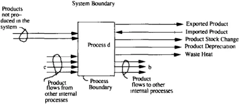
Once the system boundary in space and time has been identified, and the processes with their input and output products have been chosen, one can begin the accounting procedure. There are six distinct types of connections, in addition to the stocks, that must be identified in analyzing any ecosystem: 1. the non-produced inputs; 2. the net outputs; 3. the product use record; 4. the product production record; 5. the total output; and 6. the waste heat flows. These product flows are shown in Fig. 1.

1. The Non-produced Inputs

We distinguish here between imported/exported products made within the defined ecosystem, and imports of special products which are not made within this system. One thinks of the import of the non-produced products as a constraint on the system’s activity level. These are the products which are sometimes deemed as scarce or growth-limiting in some sense. Sunlight is a non-produced import but not the only possible one. For example,

(11)

sunlight contains blue, red. and infrared radiation, all of which may be used by the ecosystem. While we sometimes think of infrared radiation as extraneous, it is possible to define this radiation as a product within the ecosystem. If the ecologist chooses not to define it in this way, then infrared radiation should be included as a non-produced input to the system.

Ambient heating is also an input to any system. In what sense is the flow of heat through the ecosystem an important theoretical consideration? Ambient heating, from an economic point of view, is very important. The departure from some ideal standard results in a drop in the value of agricultural output and an increase in fossil fuel use. From the ecologic point of view, the heat flow is also very important, since temperature is a primary controlling factor in many life processes. However, heat flows are largely cyclical and within a given range, they are predictable. To this extent, heat flows are not of primary importance in ecosystem studies. They are of course important in detailed studies of the variations in organism development in the ecosystem. We recommend that heat flows be included as a measured net inputs to the system.

2. The Net Outputs

The net output flows are connections from the defined ecosystem across the system boundary to itself at a future time and/or to other ecosystems. There are three kinds of net output flows which must be accommodated in our accounting system.

First, we have the import and export of products made and/or used by the processes in the defined system. For example, in an aquatic ecosystem, one of the processes is likely to be algae, and one of its output products would be “algal biomass”. Some of this biomass could be washed from the system (export) or into the system (import) during a flood.

The second kind of net output flow is the change in the storage level of a particular product which occurs during the designated time period. Since we have assumed a static picture of the ecosystem, we must include the changes in stocks explicitly as flows. These flows might be thought of as flows across the time boundary of the chosen period. For example, an increase in storage will be used in the next or later time periods.

(12)

Thus, when one observes a quantity of living substance perceived to be of constant stock over the chosen time period, one is really seeing the

balanced result of the decay and replacement processes. During the study

time period, a certain amount of the living product actually decayed into its component parts and some of that lost stock was replaced. This decay-replacement process is known to occur because the products of decomposition and the net absorption of energy are both evident. If the stock size of the organism does not change during the chosen time period, what is lost or gained by the organism? It is known from thermodynamics

that the order of the structure of the organism was lost for that stock of

product which decayed during the time period. Yet, for the case where the total product stock size did not change, that lost order was exactly made up by what we call the replacement process. One must record the contribution of this replacement process in some manner. It is a product contribution across the time boundary of the system in the same manner as is the net change of a product stock.

Decay rates can be measured directly by isolating a sample of the product in question and observing the loss of order with time. Frequently this isolation is not possible or practical, however, and an estimate of the magnitude of the decay rate for living products (e.g., biomass) must be substituted. The basal metabolism of living products can be used as an estimate of decay rates, since it represents the replacement flow required

just to compensate for decay processes when the organism is at rest.

In a similar way, abiotic products in the ecosystem (e.g., solution ammonia) might also degrade during the time period, and in the process, give off heat. We need to know what the normal degradation rate would have been for this substance at the system temperature. Such data for most substances can be found in standard chemical reference handbooks. We

accept these standard data as the replacement rate of the non-living sub-

stances in question. If one wishes to account for the waste heat associated with the decomposition of these abiotic compounds, one could add another process to the accounting system which describes the input and output of the compound and its degradation (therefore its replacement rate) and record the associated waste heat. Of course, some of the non-living substances might already be at their lowest energy state, at equilibrium with the system environment (e.g., carbon dioxide), and no decay need be considered.

(13)

90 HANNON, (‘OSTANZA. AND ULANOWIC‘Z

balance of the total flow of that substance in the system. The assignment process does not double count any of the flows.

3. The Product Use Record

We have chosen the “Use” and “Make” matrices approach (Stone, 1963) and modified it to meet the special problems involved with ecological flows. The “Use” matrix is the record of which process uses what product. The “Make” matrix is the product production record and is discussed in the next section.

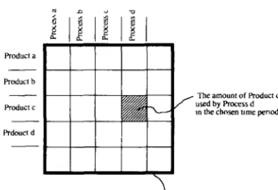
The first accounting step is to record where each product is used and by which process. A “Use” or U matrix is constructed as follows: Each process is placed at the head of a column in the U matrix; each product is placed at the beginning of a row in this matrix. The use of a product (e.g., product “c”) by a particular process (e.g., process “d”) for the chosen time period (i.e., the flow of “c” into “d”), is the number placed on the cell which lies at the intersection of row “c” and column “d”. The quantities of the substances consumed by predators for example, appear in the U matrix. The picture of the U matrix appears in Fig. 2.

The units of measure of product c must be the same wherever product c is used, but these need not be the same as the measure for any of the other products. For example, product c may be measured in grams-carbon per square meter and product d may be measured in kcal per square meter. So long as the units are consistent along the row of U, the products may be measured in any units.

It is clear to ecologists that the inputs to a particular species may vary in type and quantity with time, with age of the individuals in that species, and with the availability of resources. It is theoretically possible to include

Product a Product b

Rdoucl d

f used by F’mcers d The amount of Fmduct c ,n the chosen t,me pmcd

(14)

such variation in a single descriptive Use matrix by devising a column for each time, age, and resource condition. This matrix is then controlled by a time-varying vector of factors, each between zero and one, which select the proper portions of each of the columns involved with that species. The Make matrix (discussed below) may require a similar modification.

Besides allowing greater convenience in data gathering, the tolerance of the U matrix for any kind of unit of measure lets the experimentalists incorporate units of “service” into the matrix. For example, the pollination of flowers by bees may be measured in “pollination bee-seconds” per square meter for the chosen time period. We know that if some pollutant reduced the bee population by half, flower productivity would decrease. But there is hardly any physical transfer from bees to flowers, except that measurable by the service units of pollination. The “bee-seconds” measure is the collective visitation time spent by bees in flowers. In the U matrix,

the process plant would have “used” so many bee-seconds of pollination

service. So the term “product” as we use it here may mean an actual physi-

cal product or a service. Negative services, such as the effect of allelopathic

chemicals, can also be included.

4. Product Production Record

In the general accounting system, a second matrix is needed to show where the products are made. Such a matrix is called a “Make” or V matrix and it has the same configuration as the U matrix: the column heads are the processes and the product names are shown at the beginning of each row. The quantified list of substances produced by prey for example, are listed in the production matrix. The elements of the V matrix

are for example, the amount of product b

process d; see Fig. 3.

which is produced or made by

Product a Praduct b

Prdouct d

f made by Process d I” thechosen tune period

The “Make” or ” matrix/

(15)

92 HANNON. (‘OSTANZA. AND ULANOWICZ

The units of a product must be consistent across the row of the V and U matrix but can vary from product to product.

The products of a species or an organism in the ecosystem can vary with the available portions of the net input. For example, at various times of the year, energy, water, and nitrogen may be in short supply. Since the organism requires these inputs in fixed proportion for growth. the rate of biomass and the type and amount of excretion products will vary. A variety of vectors can be assigned to a particular organism or species and a time- varying control vector, whose zero to one factors depend on the mix of net inputs, can be used to the appropriate mix of outputs through time.

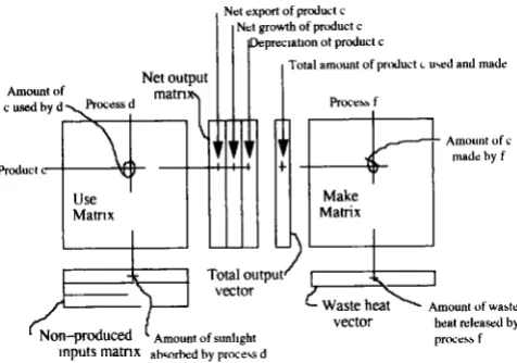
5. The Total Output Flop

The sum of the entries in a row of U plus the corresponding row of the net outputs is the total output flow for that product. This sum is also equal to the sum of the corresponding row of the V or “Make” matrix. The balance here provides a check on the various product entries.

6. The Waste Heat Flon

The respiratory or total waste heat is composed of the basal metabolic heat from the process and the organism’s muscle and bone friction, prey- seeking or predator-avoidance effort, and reproductive effort. To complete the accounting procedure, we collect all of the heat given off by each process into a vector. We consider this heat as lost to the system due to its lack of utility to any of the other organisms in the system. If some of this heat were used by certain components in the ecosystem, then that quantity of heat would be classed as a product produced and used by the appropriate components in the U and V matrices. If some of this “waste” heat could be used as a measure of reproductive service for example, then that quantity of heat would appear in the U and V matrices as used and made by the same component. All of the “waste” heat could be assigned in this manner. Note that the waste heat flow defined in this section is not associated with the basal metabolic processes: those substances representing basal metabolism have been assigned to represent the decay processes and appear in the net output.

(16)

Total amount of product L wed and made

Amount “f c mad< hy f

Amount of wastr

heat drascd by

prOCeS5 f

FIG. 4. The general accounting system describing the assignment of all product flows to where they are made and used.

tabulated at the bottom edge of the V (Make) matrix as a notational reminder that they have been accounted for. The complete ecological accounting system therefore looks as shown in Fig. 4.

As a matter of accounting convenience, the U and V matrices are overlaid in tabular form and kept in the same table, with the Make or V matrix entries shown immediately below the Use or U matrix entries. Also note that the U and V matrices will most likely be rectangular and not square, because the number of products used will not necessarily equal the number of products made.

The general accounting procedure is shown in the following examples.

D. Examples

The following simplified examples will serve to illustrate the accounting system. We have chosen to use simplified examples rather than data from actual systems. The application of a simplified form of the accounting system to the Southern North Sea ecosystem has been published (Hannon and Joiris, 1989; Costanza and Hannon, 1989). Our goal in this paper is to demonstrate the full accounting system in the simplest possible form so that each of the principles can be clearly explained. We know of no ecosystem for which a sufftcient amount of data has been collected and codified for application of the full accounting procedure.

(17)

TABLE 1 Hypothetical Ecosystem Network Illustrating the General Accounting Framework

Products (units)

Internal Processes External Processes Net Outputs Abiotic Biotic processes Chemical Change in Exports/ Depre- Processes Producers Consumers stock imports ciatlon Nutrients use (g/t)

make stock

Plant

biomass

use

(g/t)

make stock

Ammal

biomass

use

(g/t)

make stock

Waste heat use (Cal/r) make Sunlight use (Cal/O make Internally produced 20 IO 0 0 5 2 20 5 5 - 7 500 0 0 - 1 5 6 1 0 1 0 I4 0 0 0 loo 0 - I I 5 0 I 0 0 8 - 0 0 0 IO - - 100 5 50 45 Externally produced 0 loo 0 - 100 Totals

(18)

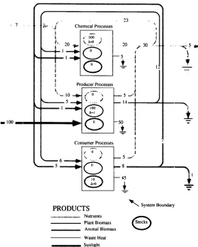
puts, and “stock” of each of these products by (or in) each of the internal processes are shown in table I and Fig. 5. The table and figure are equivalent representations of the system. Figure 6 shows the nutrient product flows isolated from the system. Most network analysis in ecosystems has in the past concentrated on just such a one-product abstraction of the system. Our general accounting framework is intended to take more of the full complexity of ecological networks into account as shown in Fig. 5 and table I.

f

23 ,. ,& .J” _Chemxal _Processes 1.

I

I Consumer I- Processes I

PRODUCTS \ System Boundary

NUtMIltS

Plant Biomass

0

Stocks Ammal Biomass

Waste Heat P Sunltght

(19)

Consumer Processes 0

r-l

5 -.

PRODUCTS Nutrients

\ System Boundary

0

Stocks

FIG. 6. Hypothetical ecosystem flows and stocks of the single product “nutrients”.

Table I represents a particularly compact, yet easily readable representa- tion of the complex flows shown in Fig. 5. For example, one can read from Fig. 5 that abiotic chemical processes use 20 g per unit time of nutrients, primary producers use 10, and consumers use 0. Nutrients are “made” by all three processes, since plants and animals release nutrients when they die and decompose. In contrast, plant and animal biomass are “made” only by producers and consumers, respectively.

(20)

system and is not made anywhere in the system. Any product that is not produced anywhere in the system under study but is necessary for the system’s survival is called an externally produced product.

There are also three “external processes” shown, change in stock, exports/imports, and depreciation replacement, along with their use and make of the system’s products. As already mentioned, a change in stock is equivalent to an export to another time period, and depreciation is equivalent to export from the system. So, taken together, these three external processes represent net outputs from the system of one kind or another.

Note that for this system (and for any system) mass and energy balance are maintained for each product. For example the total use of nutrients in the system of 37 g/t (use by internal processes plus use by external processes in the form of change in stock, exports and depreciation) is equal to the total production of nutrients by internal processes plus imports (also 37 g/r). Product use must balance product make for each product in the system.

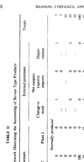
“Products” in our accounting system can also be services or information. To illustrate this we present an example system in which bee pollination services are an important product (table II). In this example the products are bee biomass, honey, plant biomass, and been pollination effort, in addition to the ubiquitous waste heat and sunlight. The internal processes are bees, and two species of plants that the bees pollinate. Bees in this system produce four different products; (1) bee biomass (7 g/r); (2) honey (35 g/t); (3) pollination effort (10 bee s/t); and waste heat (5 Cal/t). Note that both bee biomass and honey are used and made exclusively by bees. Bee pollination effort is used more by plant 1 (6 bee s/t) than by plant 2 (3 bee s/t). Plant 1 also has twice the biomass stock of plant 2 (200 vs. 100) and uses more sunlight (40 vs. 30 Cal/r).

E. Data Quality Control

(21)

TABLE II Hypothetical Ecosystem Network Illustrating the Accounting of Service Type Products

Products (units)

Bees Internal processes Plant I Plant 2 External processes Totals Net outputs Change in exports/ Depre- stock Imports ciation Bee biomass

(g/O Honey k/Q Plant

biomass

(g/t) Bee

pollination

Effort (bee

s/r) use 5 0 make 7 0 stock 35 0 use 30 0 make 35 0 stock 0 100 use 5 25 make 0 33 stock 0 200 use 0 6 make 10 0 stock IO 0 Internally produced

0 0 0 0 0 0 ₃₅ ₄₀

100 3 0 0

I

0 0

0

0 0

0

3

0

-

0 0 0

1

7 7 g

j

3.5 ci

5

35 35

- 2 0 100 =r 5 73 0 73 5 - 300 % I

10 10

2

10

* r;r

Waste

heat

(CW Sunlight (Wr) use make use make

(22)

ACCOUNTING FOR ECOLOGICALSYSTEMS 99

system, once a number is obtained and exported to the general scientific community it is labelled either “good” or “bad,” and the record of its degree of quality is all but forgotten except by the experts familiar with the details of the measurement methods. What is needed is a formal, systematic way of communicating to the non-expert the “degree of goodness” or “quality” associated with each number. This can be imagined as composed of its degrees of precision and accuracy; that is, how little “spread” or scatter there is in its underlying data, and how reliable it is as an estimate of what it is measuring. Thus, we can think of all quantitative measurements as having associated truth-value modifiers, which we will call the “grades” of numbers. We chose this term since everyone is familiar with the grading process through their academic experience, and the process of grading quantitative measurements is conceptually similar to grading students or grading almost anything else. Also, stating a grade with each number connotes the evaluative and qualitative nature of the measure of uncertainty we propose, which is in keeping with its correct interpretation,

Such systems for grading and manipulating data of sub-statistical quality are currently under development (e.g., ‘Funtowitz and Ravitz, 1989). We lack the space to adequately treat them here, except to say that they are a necessary adjunct to the proposed accounting system to allow information the qualify of numerical estimates to be carried through the accounting and subsequent manipulations of complex systems built up from measurements of highly varying quality. They will ultimately allow a more honest and rational use of our numerical resources.

IV. USES OF THE GENERAL ACCOUNTING SYSTEM

The accounting framework described above allows the collection of ecosystem data in a form that is useful for a number of analytical purposes. Some of these uses and their importance are described in detail in a number of recent works (e.g.) Hannon and Joiris, 1989, Costanza and Hannon, 1989, Fasham, 1984; Hannon, 1986; MacDonald, 1983; Ulanowicz, 1986; and Wulff et al., 1989). Below we briefly describe some examples that demonstrate existing and potential uses, but the presence of a consistent accounting framework should allow an explosion of new uses not mentioned or conceived of here.

(23)

100 HANNON. COSTANZA. AND ULANOWICZ

A. Network Ana!,~sis and Energy Itltensities

The “mixed units” problem is a crltical one in both ecology and economics. We have elaborated an accounting system which allows multiple products, but most analytical work requires (or at least is much more convenient) when only a single product is tracked. One area of research therefore is the conversion of the full multi-product network into an equivalent single-product network. Work in this area has so far centered on various ways to calculate intensity factors (analogous to prices in economic systems) that allow all the system’s products to be converted into a common currency (Hannon, Costanza, and Herendeen, 1986; Hannon and Costanza, 1985, Costanza, and Hannon, 1989). If the system under study has only one non-produced input (usually sunlight for ecological systems) and there are an equal number of products and processes it becomes possible to calculate the input intensities that represent the amount of the non-produced input “embodied” in each of the system’s products (Costanza and Hannon, 1989). These energy intensities can then be used to convert the system into a single product network (i.e., in “embodied sunlight”) that is amenable to further network analysis. The range of possible network analysis that can be performed on single product ecologi-

cal networks is given in a recent compendium (Wulff et al., 1989).

The general accounting framework will also allow analysis of different but connected geographical ecosystems. The matrix of use and make for the first ecosystem would be arranged in the manner stated above. The use matrix of the second, adjoining ecosystem would be appended to the use matrix of the first one, centered on the extended diagonal of the lirst. Any exchanges between the two ecosystems would be placed in the appropriate cell in the matrix to the right of or below the first matrix. The vectors of net and total output and of net input of the first matrix would be extended in length to accommodate those same vectors from the second system. The combined result could then be analyzed as though it were a single system matrix. For example, the above mentioned energy intensities would then reflect the combination of the two systems with possibly differing intensities for the same product from each system.

B. Simulation Modeling

(24)

Ecosystem simulation has been by far the most popular form of analysis of whole ecosystems. Thousands of ecosystem simulation models have been constructed over the years and we could not begin to summarize them here. Most of these modeling studies involved using either an explicit or an implicit, ad hoc accounting framework as a preliminary step. Our point is that the proposed framework will provide a consistent base from which to start, a minimum ideological baggage, and a minimum of unnecessary duplication of data collection. This step would facilitate ecosystem modeling of all kinds.

C. Optimization

Network analysis, simulation, and the related techniques help to portray the effects of the entire system upon individual processes and product flows.

But the data required by energy budgets also can be used to gauge how the

system as a whole is acting. In order to quantify such system tendencies some investigators have attempted to formulate objective functions that might portray some overall preferred state or goal. For example, H. T. Odum (1971) placed great stress on the maximization of useful output as a criterion for a population’s survival (an idea which has much earlier been articulated by Lotka (1922)). Odum suggested that the Lotka maximum power principle also might be applicable to the ecosystem in aggregate. Hannon (1979) and Hannon et al. (1986) have posited that the scalar product of the energy intensities with the net outputs of each system is an appropriate objective function.

Ulanowicz (1980, 1986) defined the network “ascendency” as an appropriate objective function. It is calculated entirely from the exchanges transpiring among the system elements and with their environment. Ascendency is purported to rise monotonically as the system grows and develops.

Fontaine (1981), Loehle (1988), and Herendeen (1991) have attempted to compare the efficacies of the various objective functions as descriptors of

system development, but to date, there is no agreement as to the best

quantitative description of system development. The problem in comparing the various whole-system hypotheses has been a paucity of data on exchanges and storages in actual ecosystems. The potentially enormous advantages resulting from the discovery of a principle for ecosystem development should highlight the urgent need for more data collected under the accounting schema described above.

(25)

102 HANNON. COSTANZA. AND ULANOWICZ

V. SUMMARY AND CONCLUSIONS

We have elaborated the need for and style of a general accounting system as an ecological research tool. When field ecologists investigate one portion of a large ecosystem, they usually design their own research strategy. In so doing, they may miss the opportunity to significantly aug- ment the future work of other scientists by slight changes in their research strategy. They may also leave off some stock or flow measurement which was unimportant to their own needs. By reviewing their research proposal and checking it against the requirements of a general accounting system, these scientists are assuring themselves that their work will be in a form usable to others. In this way, their research is contributing to a network of understanding of the larger ecosystem. As the research progresses on the pieces of the larger system, the time approaches when they and other scientists will be able to synthesize the collective information into a model of the larger system function.

ACKNOWLEDGMENTS

The authors thank Craig Loehle and G. A Swanson for thetr useful comments.

REFERENCES

AMIR, S. 1979. Economic interpretattons of equthbrmm concepts in ecological systems, J. Sot.

Biol. Struct. 2, 293-314.

AMIR, S. 1987. Energy pricing, btomass accumulation, and project appraisal, in “Environmen- tal Economics: The Analysis of a Major Interface” (G. Pillet and T. Murota, Eds.), pp. 53-103, Leimbreger, Geneva.

BAIRD, D., AND ULANOWICZ, R E. 1989. The seasonal dynamtcs of the Chesapeake Bay ecosystem, Ecol. Monographs 59(4), 329-364.

BARBER, M. 1978. A retrospecttve Markovtan model for ecosystem resource flow, Ecol. Model

5, 125-35.

BULLARD, C.. SEBALD, A. 1977 Effects of parametric uncertamty and technologmal change on input-output models, Reo. Econ. Stat. 59(l), 75-81.

COSTANZA, R. 1980. Embodied energy and economic valuatton, Scrence 210, 1219-1224. COSTANZA, R., AND HERENDEEN, R. A. 1984. Embodied energy and economic value in the

United States economy: 1963, 1967, and 1972, Resow. Energy 6, 129-164.

COSTANZA. R., AND NEILL, C. 1984. The energy embodied in the products of ecological systems: a lmear programming approach, J. Theor. Biol. 106, 41-57.

(26)

COSTANZA, R., AND HANNON, B. 1989. Dealing with the “mIxed” units problem in ecosystem analysis, in “Flow Analysis of Marine Ecosystems” (F. Wulff, J. G. Field, and K. H. Mann, Eds.), Chap. 5, Ecological Studies Series, Springer-Verlag, Berlin/New York. DALY. H. 1968. Economics as life science, J. Polit. Econ. 76, 392401.

FASHAM, M. J. R. 1984. “Flows of Energy and Materials in Marme Ecosystems,” Plenum, New York.

FINN, J. 1976. Measure of ecosystem structure and function derived from the analysis of flows,

J. Theor. Biol. 56, 363-380.

FONTAINE, T. D. 1981. A self-designing model for testmg hypotheses of ecosystem development, in “Progress in Ecological Engineering and Management by Mathematical Modelling” (S. E. Jorgensen, Ed.), pp. 281-291, Elsevier, Amsterdam.

FUNTOWITZ, S., AND RAVITZ, J. 1989. “Uncertainty and Quality m Science for Pohcy,” Kluwer, Amsterdam.

HANNON, B. 1973. The structure of ecosystems, J. Theor. Biol. 41, 535-546.

HANNON, B. 1979. Total energy costs in ecosystems, J. Theor. Biol. 80, 271-93.

HANNON, B. 1986. Ecosystem control theory, J. Theor. Biol. 121, 417437.

HANNON, B. M., AND COSTANZA, R. 1985. Ecosystems with multiple products. ISEM Journal 7, 2749.

HANNON, B., COSTANZA, R , AND HERENDEEN, R. 1986. Measures of energy cost and value in ecosystems, J. Enoiron. Econ. Management 13, 391401.

HANNON, B., AND JOIRIS, C. 1989. A seasonal analysis of the Southern North sea ecosystem,

Ecology 70(6), 19161934.

HERENDEEN, R. 1991. Do economics-like principles predict ecosystem behavior under changing resource constraints? in “Theoretical Studies Ecosystems: The Network Perspective” (T. Bums and M. Higashi, Eds), pp. 261-287, Cambridge Univ. Press.

KOOPMANS, f. C. (Ed.) 1951. “Activity Analysis of Productron and Allocation,” Wiley, New York.

KUZNETS, S. 1946. Problems of interpretation of national accounts, in “National Income: A Summary of Findings,” pp. I1 1-129, National Bureau of Economic Research, New York. LEONTIEFF. W. 1941. “The Structure of the American Economy, 1919-1939,” Oxford Univ.

Press, New York.

LINDEMAN. R. L. 1942. The trophicdynamic aspect of ecology, Ecology 23, 399418. LOEHLE, C. 1988. Evolution: The missing ingredient in systems ecology, Amer. Naf. 132,

884-899.

LOTKA, A. J. 1922. Contribution to the energetics of evolution, Proc. Narl. Acad. Ser. U.S.A.

8, 147-155.

MACDONALD, N. 1983. “Trees and Networks in Biological Models,” Wiley, Chichester. MATIS, J. H., AND PATTEN, B. C. 1981. Environ analysis of linear compartmental systems: The

static, time Invariant case, Bull. Int. Stat. Inst. 48, 527-565.

ODUM, E. P. 1953. “Fundamentals of Ecology,” Saunders, Philadelphia. ODUM, H. T. 1971. “Environment, Power, and Society,” Wiley, New York.

ODUN, E. P., AND ODUM, H. T. 1959.” Fundamentals of Ecology,” 2nd ed., Saunders, Philadelphia.

ODUM, H. T., AND PINKERTON, R. C. 1955. Time’s speed regulator: The optimum efficiency for maximum power output in physical and biological systems, Amer. Sci. 43, 331-343.

PATTERN, B., BOSSERMAN, R., FINN, J. AND CALE, W. 1976. Propagation of cause m ecosystems, in “Systems Analysis and Simulation in Ecology,” Vol. 4, pp. 457479, Academic Press, New York.

ROUGHGARDEN, J., 1989, The U.S. needs an ecological survey, Bioscience 39( 1), 5.

(27)

STONE. R 1963. Input-output relattonships 1954-1966. ~1 “A Programme for Growth.” Vol. 3, pp. 11-22, MIT Press. Cambridge, MA

ULANOWICZ. R. E. 1980. An hypothesrs on the development of natural communities. J. Thm Bid. 85, 223-245.

ULANOWICZ. R. E. 1986. “Growth and Development, Ecosystems Phenomenology,” Springer- Verlag. New York.

ULANOWICZ, R.. AND KEhlP, W. 1979 Toward canomcal trophtc aggregatton, Amer. A’at. 114. 871-883.