Deep Exploration via Randomized Value Functions
Ian Osband [email protected]
DeepMind
Benjamin Van Roy [email protected]
Stanford University
Daniel J. Russo [email protected]
Columbia University
Zheng Wen [email protected]
Adobe Research
Editor:Peter Auer
Abstract
We study the use of randomized value functions to guide deep exploration in reinforcement learning. This offers an elegant means for synthesizing statistically and computationally efficient exploration with common practical approaches to value function learning. We present several reinforcement learning algorithms that leverage randomized value functions and demonstrate their efficacy through computational studies. We also prove a regret bound that establishes statistical efficiency with a tabular representation.
Keywords: Reinforcement learning, exploration, value function, neural network
1. Introduction
Reinforcement learning might provide the basis for an artificial intelligence that can manage a wide range of systems and better serve the needs of society. To date, its potential has primarily been assessed through learning in simulated systems, where data generation is relatively unconstrained and algorithms are routinely trained over millions to trillions of episodes. Real systems, where data collection is costly or constrained by the physical context, call for a focus on statistical efficiency. A key driver of statistical efficiency is how the agent explores its environment.
The design of reinforcement learning algorithms that efficiently explore intractably large state spaces remains an important challenge. Though a substantial body of work addresses efficient exploration, most of this focusses on tabular representations in which the number of parameters learned and the quantity of data required scale with the number of states. Despite valuable insights that have been generated through design and analysis of tabular reinforcement learning algorithms, they are of limited practical import because, due to the curse of dimensionality, state spaces in most contexts of practical interest are enormous. There is a need for algorithms that generalize across states while exploring intelligently to learn to make effective decisions within a reasonable time frame.
In this paper, we develop a new approach to exploration that serves this need. We build on value function learning, which underlies the most popular and successful approaches to reinforcement learning. In common value function learning approaches, the agent maintains
a point estimate of a function mapping state-action pairs to expected cumulative future reward. This estimate typically takes a parameterized form, such as a linear combination of features or a neural network, with parameters fit to past observations. The estimate approximates the agent’s prevailing expectation of the true value function, and can be used to guide action selection. As actions are applied and new observations gathered, parameters are adapted to fit the growing data set. The hope is that this process quickly converges on a mode in which the agent selects near optimal actions and new observations reinforce prevailing value estimates.
In using the value function estimate to guide actions, the agent could operate according to a greedy policy, which at any given state, applies the action that maximizes estimated value. However, such a policy does not investigate poorly-understood actions that are assigned unattractive point estimates. This can forgo enormous potential value; it is worth-while to experiment with such an action since the action could be optimal, and learning that can provide cumulating future benefit over subsequent visits to the state. Thoughtful exploration can be critical to effective learning.
The simplest and most widely used approaches to exploration perturb greedy actions with random dithering. An example is -greedy exploration, which selects the greedy ac-tion with probability 1− and otherwise selects uniformly at random from all currently available actions. Dithering induces the experimentation required to learn about actions with unattractive point estimates. However, such approaches waste much exploratory ef-fort because they do not “write-off” actions that are known to be inferior. This is because exploratory actions are selected without regard to the level of uncertainty associated with value estimates. Clearly, it is only worth experimenting with an action that is expected to be undesirable if there is sufficient uncertainty surrounding that assessment. As we will discuss further in Section 4, this inefficiency can result in learning times that grow exponentially with the number of states.
A more sophisticated approach might only experiment with an action when applying the action will reveal useful information. We refer to such approaches asmyopic, since they do not account for subsequent learning opportunities made possible by taking an action. Though myopic approaches do “write off” actions where dithering approaches fail to, as we will discuss in Section 4, myopic exploration can also require learning times that grow exponentially with the number of states or even entirely fail to learn.
Reliably efficient reinforcement learning calls for deep exploration. By this we mean that the exploration method does not only consider immediate information gain but also the consequences of an action on future learning. A deep exploration method could, for example, choose to incur losses over a sequence of actions while only expecting informative observations after multiple time periods. Dithering and myopic approaches do not exhibit such strategic pursuit of information.
There is much more to be said about the design of algorithms that leverage randomized value functions, and we cover some of this ground in Section 5. It is worth mentioning here, though, that this concept is abstract and broadly applicable, transcending specific algorithms. Randomized value functions can be synthesized with the multitude of useful algorithmic ideas in the reinforcement learning literature to produce custom approaches for specific contexts.
To provide insight into the efficacy of randomized value functions, in Section 6, we establish a strong bound on the Bayesian regret of a tabular algorithm. This is not the first result to establish strong efficiency guarantees for tabular reinforcement learning. However, previous algorithms that have been shown to satisfy similar regret bounds do not extend to contexts involving generalization via parameterized value functions. In this regard, the approach we present is the first to satisfy a strong regret bound with tabular representations while also working effectively with the wide variety of practical value function learning methods that generalize over states and actions.
Section 7 presents computational results guided by randomized value functions that synthesize efficient exploration with generalization. Experiments with a family of simple toy examples demonstrate dramatic efficiency gains relative to dithering approaches for exploration and that our randomized approaches are compatible with linearly parameterized generalizing value functions. We also consider a cart-pole balancing problem that requires both deep exploration and generalization. We address this problem through a combination of randomization and deep learning, with value functions represented by neural networks.
2. Literature review
The Bayes-optimal policy serves as a gold standard for statistically efficient exploration in reinforcement learning (RL). Given a prior distribution over Markov decision processes, one can formulate a problem to maximize expected cumulative reward by taking an action at each future time contingent on the prevailing posterior distribution. A policy that attains this maximum is Bayes-optimal, and to do this it must explore judiciously. Unfortunately, for problems of practical interest, computing a Bayes-optimal policy is intractable; the com-putational requirements grow exponentially in the problem parameters (Szepesv´ari, 2010). We introduce an approach based on randomized value functions that offers a computa-tionally tractable approach to statistically efficient reinforcement learning. Exploration via randomized value functions is not generally Bayes-optimal but, as we will argue, offers a practical approach to deep exploration, which common exploration schemes fail to address, sometimes at enormous cost to statistical efficiency.
bound the level of sub-optimality by some polynomial function of states and/or planning horizon. By contrast, popular schemes such as -greedy and Boltzmann exploration can require learning times that grow exponentially in the number of states and/or the planning horizon (see, e.g., Kakade (2003); Strehl (2007)). We discuss this phenomenon further in Section 4.
The design and analysis of tabular algorithms has generated valuable insights, but the resultant algorithms are of little practical importance since, for practical problems the state space is typically enormous (due to the curse of dimensionality). To learn effectively, prac-tical RL algorithms must generalize across states to make effective decisions with limited data. The literature offers a rich collection of such algorithms (e.g. Bertsekas and Tsit-siklis (1996); Sutton and Barto (2018); Szepesv´ari (2010); Powell and Ryzhov (2011) and references therein). Though algorithms of this genre have achieved impressive outcomes, notably in games such as backgammon (Tesauro, 1995), Atari arcade games (Mnih et al., 2015), and go (Silver et al., 2016, 2017), they use naive exploration schemes that can be highly inefficient. Possibly for this reason, these applications required enormous quantities of data. In the case of Silver et al. (2016), for example, neural networks were trained over hundreds of billions to trillions of simulated games.
The design of reinforcement learning algorithms that efficiently explore intractably large state spaces remains an important challenge. Model learning algorithms exploit gener-alization in an underlying model of the environment (Kearns and Koller, 1999; Abbasi-Yadkori and Szepesv´ari, 2011; Ibrahimi et al., 2012; Ortner and Ryabko, 2012; Osband and Van Roy, 2014a,b; Gopalan and Mannor, 2015). However, these are typically restricted to simple model classes and become statistically or computationally intractable for problems of practical scale. Policy learning algorithms, and the closely-related ‘evolutionary’ algo-rithms identify high-performers among a set of policies (Kakade, 2003; Wierstra et al., 2008; Deisenroth et al., 2013; Plappert, 2017). These algorithms can perform well, particularly when the space of possible optimal policies is parameterized to be small. However, in a typ-ical problem the space of policies is exponentially large; existing works either entail overly restrictive assumptions or do not make strong efficiency guarantees.
Value function learning has the potential to overcome computational challenges and offer practical means for synthesizing efficient exploration and effective generalization. A relevant line of work establishes that efficient reinforcement learning with value function generalization reduces to efficient “knows what it knows” (KWIK) online regression (Li and Littman, 2010; Li et al., 2008). However, it is not known whether the KWIK online regres-sion problem can be solved efficiently. In terms of concrete algorithms, there is optimistic constraint propagation (OCP) (Wen and Van Roy, 2013), a provably efficient reinforce-ment learning algorithm for exploration and value function generalization in deterministic systems, and C-PACE (Pazis and Parr, 2013), a provably efficient reinforcement learning algorithm that generalizes using interpolative representations. These contributions repre-sent important developments, but OCP is not suitable for stochastic systems and is highly sensitive to model misspecification, and generalizing effectively in high-dimensional state spaces calls for methods that extrapolate.
Wen (2014). Prior reinforcement learning algorithms that generalize via parameterized value functions require, in the worst case, learning times exponential in the number of model pa-rameters and/or the planning horizon. RLSVI aims to overcome these inefficiencies. While RLSVI operates in a manner similar to well-known approaches such as least-squares value iteration (LSVI) and SARSA (see, e.g. Sutton and Barto (2018)), what fundamentally distinguishes RLSVI is exploration through randomly sampling statistically plausible value functions. Alternatives such as LSVI and SARSA are typically applied in conjunction with action-dithering schemes such as Boltzmann or -greedy exploration, which lead to highly inefficient learning.
This paper aims to establish the use of randomized value functions as a promising approach to tackling a critical challenge in reinforcement learning: synthesizing efficient ex-ploration and effective generalization. The only preceding work that advocates exex-ploration through random samples of the value function comes from Dearden et al. (1998). This paper proposes a tabular algorithm that resamples every timestep and so does not perform deep exploration. A preliminary version of part of this work appeared in a short conference paper (Osband et al., 2016b). While that paper proposed a specific algorithm that is compatible with linear function approximation, this paper develops the concept of deep exploration via randomized value functions in much greater depth and generality. We provide a gen-eral template for building algorithms that perform randomized value function learning and propose several specific instantiations of this idea. These algorithms are evaluated in en-tirely new simulations experiments, including an example in which neural networks are used for function approximation. While a proof sketch for a regret bound was given in (Osband et al., 2016b), this paper gives a full and careful proof and develops new recursive stochastic dominance arguments that simplify the analysis. Following (Osband et al., 2016b), several papers have proposed adaptations to neural network function approximation via bootstrap sampling (Osband et al., 2016a), linear final layer approximation (Azizzadenesheli et al., 2018) or variational inference (Lipton et al., 2018; Fortunato et al., 2018).
The mathematical analysis we present in Section 6 establishes a bound on expected regret for a tabular version of RLSVI applied to an episodic finite-horizon problem, where the expectation is taken with respect to a particular uninformative distribution. We view this result as a sanity check that, although it is designed for exploration with generalization, RLSVI recovers state-of-the-art efficiency guarantees in the simple tabular setting. Our bound is ˜O(H
√
SAHL), where S and A denote the cardinalities of the state and action spaces,Ldenotes the number of episodes elapsed, andHdenotes the episode duration. The lower bound of Jaksch et al. (2010) can be adapted to the episodic finite-horizon context to produce a Ω(H
√
SAL) lower bound that applies to any algorithm. This differs from our upper bound by a factor of
√
H, though this is not an apples-to-apples comparison, since the lower bound applies to a maximum over Markov decision processes and may not hold for the expectation over Markov decision processes, taken with respect to a prior distribution we posit. Follow up work by Russo (2019) shows that RLSVI also satisfies worst-case regret bounds in tabular environments.
is aligned with the task objective. Crucially, this generalization is not learned from the task and, unlike the optimal value function, “counts” are generated by the agent’s choices so there is no single target function to learn. Further, these approaches add uncertainty bonus that is uncoupled across states, which can lead to a substantial negative impact on statistical efficiency, as discussed in (Osband and Van Roy, 2017; O’Donoghue et al., 2017). Exploration via randomized value functions is inspired by Thompson sampling (Thomp-son, 1933; Russo et al., 2018). In particular, when generating a randomized value function, the aim is to approximately sample from the posterior distribution of the optimal value function. There are problems where Thompson sampling is in some sense near-optimal (Agrawal and Goyal, 2012, 2013a,b; Russo and Van Roy, 2013, 2014a; Gopalan and Man-nor, 2015). Further, the theory suggests that “well-designed” upper-confidence-bound-based approaches, which appropriately couple uncertainties across state-action pairs, but are of-ten computationally intractable, are similarly near-optimal (statistically) and competitive with Thompson sampling in such contexts (Russo and Van Roy, 2013, 2014a). On the other hand, for some problems with more complex information structures, it is possible to explore much more efficiently than do Thompson sampling or upper-confidence-bound methods (Russo and Van Roy, 2014b). As such, for some RL problems and value function representations, the randomized value function approaches we put forth will leave substan-tial room for improvement.
At a high level, randomized value functions replaces a point estimate of the value func-tion by a distribufunc-tion of plausible value funcfunc-tions. Recently, another approach called “dis-tributional RL” also suggests replacing a scalar value estimate by a distribution (Bellemare et al., 2017). Although both might reasonably claim to offer a distributional perspective on reinforcement learning, the meaning and utility of the two distributions are quite distinct. Randomized value functions aim to sample from a distribution that captures the Bayesian uncertainty in the unknown optimal value function; this concentrates around the true value function as more data is gathered. By contrast, “distributional RL” fits a distribution to the realized value under stochastic outcomes. For efficient exploration of unknown rather than stochastic outcomes, it is important to use the correct notion of “distributional RL”.
3. Reinforcement learning problem
We consider a reinforcement learning problem in which an agent interacts with an unknown environment over a sequence of episodes. We model the environment as a Markov decision process, identified by a tuple M = (S,A,R,P, ρ). Here, S is a finite state space, A is a finite action space,Ris a reward model,P is a transition model, andρ∈ S is an initial state distribution. For each s, ρ(s) is the probability that an episode begins in state s. For any s, s′∈ S anda∈ A,Rs,a,s′ is a distribution over real numbers andPs,a is a sub-distribution over states. In particular, Ps,a(s′) is the conditional probability that the state transitions tos′ from statesand actiona. Similarly,Rs,a,s′(dr) is the conditional probability that the
reward is in the set dr. By sub-distribution, we mean that the sum can be less than one. The difference 1− ∑s′∈SPs,a(s′)represents the probability that the process terminates upon
transition.
state s`0 ∼ ρ and selects an action a`0 ∈ A. Given this state-action pair, a reward and transition are generated according to r1` ∼ Rs`
0,a
`
0,s
`
1 and s
`
1 ∼ Ps`
0,a
`
0. The agent proceeds
until termination, in each tth time period observing a state s`t, selecting an action a`t, and then observing a reward rt`+1 and transition to s`t+1. Let τ` denote the random time at
which the process terminates, so that the sequence of observations made during episode ` isO`= (s`0, a`0, r`1, s`1, a`1, . . . , s`τ
`−1, a
` τ`−1, r
` τ`).
We define a policy to be a mapping from S to a probability distribution over A, and denote the set of all policies by Π. We will denote byπ(a∣s)the probability thatπ assigns to action a at state s. Without loss of generality, we will consider states and actions to be integer indices, so that S = {1, . . . ,∣S ∣} and A = {1, . . . ,∣A∣}. As such, we can define a substochastic matrix whose(s, s′)th element is∑a∈Aπ(a∣s)Ps,a(s′). We make the following assumption to ensure finite episode duration:
Assumption 1 For all policies π ∈Π, if each action at is sampled from π(⋅∣st), then the
MDP M almost surely terminates in finite time. In other words, limt→∞Pπt=0, where Pπ
is the matrix whose (s, s′)th element is ∑a∈Aπ(a∣s)Ps,a(s′).
For any MDP Mand policyπ∈Π, we define a value function VMπ ∶ S ↦R by
VMπ(s) =EM,π[
τ
∑
t=1
rt ∣s0=s],
where rt, st, at, and τ denote rewards, states, actions, and termination time of a generic
episode, and the subscripts of the expectation indicate that actions are sampled according to at ∼ π(⋅∣st) and transitions and rewards are generated by the MDP M. Further, we define an optimal value function:
VM∗ (s) =max
π∈Π V
π
M(s).
The agent’s behavior is governed by a reinforcement learning algorithm alg. Immediately prior to the beginning of episode L, the algorithm produces a policy πL=alg(S,A,HL−1) based on the state and action spaces and the history HL−1 = (O`∶`=1, . . . , L−1) of ob-servations made over previous episodes. Note that alg may be a randomized algorithm, so that multiple applications of alg may yield different policies.
In episode`, the agent enjoys a cumulative reward of ∑τt=`1rt`. We define theregretover episode`to be the difference between optimal expected value and the expected value under algorithm alg. This can be written as EM,alg[V∗(s`0) −Vπ
`
(s`0))], where the subscripts of the expectation indicate that each policy π` is produced by algorithm alg and state transitions and rewards are generate by MDP M. Note that this expectation integrates over all initial states, actions, state transitions, rewards, and any randomness generated within alg, while the MDPMis fixed. We denotecumulative regret overL episodes by
Regret(M,alg, L) =
L
∑
`=1
EM,alg[V∗(s`0) −Vπ
`
When used as a measure for comparing algorithms, one issue with regret is its depen-dence onM. One way of addressing this is to assume thatMis constrained to a pre-defined set and to design algorithms with an aim of minimizing worst-case regret over this set. This tends to yield algorithms that behave in an overly conservative manner when faced with representative MDPs. An alternative is to aim at minimizing an average over representative MDPs. The distribution over MDPs can be thought of as a prior, which captures beliefs of the algorithm designer. In this spirit, we defineBayesian regret:
BayesRegret(alg, L) =E[Regret(M,alg, L)].
Here, the expectation integrates with respect to a prior distribution over MDPs.
It is easy to see that minimizing regret or Bayesian regret is equivalent to maximiz-ing expected cumulative reward. These measures are useful alternatives to expected cu-mulative reward, however, because for reasonable algorithms, Regret(M,alg, L)/L and BayesRegret(alg, L)/L should converge to zero. When it is not feasible to apply an op-timal algorithm, comparing how quickly these values diminish and how that depends on problem parameters can yield insight.
To denote our prior distribution over MDPs, as well as distributions over any other randomness that is realized, we will use a probability space (Ω,F,P). With this notation, the probability that M takes values in a set M is written as P(M ∈ M). In fact, the probability of any measurable eventE is written asP(E ).
4. Deep exploration
Reinforcement learning calls for a sophisticated form of exploration that we refer to as
deep exploration. This form of exploration accounts not only for information gained upon taking an action but also for how the action may position the agent to more effectively acquire information over subsequent time periods. We will use the following simple example to illustrate the critical role of deep exploration as well as how common approaches to exploration fall short on this front.
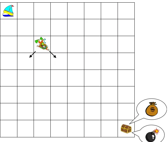
Example 1 (Deep-sea exploration)
Consider an MDPM = (S,A,R,P, ρ) with∣S ∣ =N2 states, each of which can be thought of
as a square cell in anN×N grid, as illustrated in Figure 1. The action space isA = {1,2}.
At each state, one of the actions represents “left” and the other represents “right,” with the indexing possibly differing across states. In other words, for a pair of distinct statess, s′∈ S,
action 1 could represent “left” at state s and “right” at state s′. Any transition from any state in the lowest row leads to termination of the episode. At any other state, the “left” action transitions to the cell immediately to the left, if possible, and below. Analogously, the “right” action transitions to the cell immediately to the right, if possible, and below. The agent begins every episode in the upper-left-most state (where her boat sits). Note that, given the dynamics we have described, each episode lasts exactly N time periods.
From any cell along the diagonal, there is a cost of0.01/N incurred each time the “right”
Figure 1: Deep-sea exploration: a simple example where deep exploration is critical.
“right” action is selected at that cell. Conditioned on the M, this reward is deterministic,
so once the agent discovers whether there is treasure or a bomb, she knows in subsequent episodes whether she wants to reach or avoid that cell. In particular, given knowledge ofM,
the optimal policy is to select the “right” action in every time period if there is treasure and, otherwise, to choose the “left” action in every time period. Doing so accumulates a reward of0.99if there is treasure and0 if there is a bomb. It is interesting to note that a policy that randomly explores by selecting each action with equal probability is highly unlikely to reach the chest. In particular, the probability such a policy reaches that cell in any given episode is (1/2)N. Hence, the expected number of episodes before observing the chest’s content is 2N. Even for a moderate value of N =50, this is over a quintillion episodes.
Let us now discuss the agent’s beliefs, or state of knowledge, about the MDP M, prior
to the first episode. The agent knows everything about Mexcept:
• Action associations. At each state, the agent does not know which action index is associated with “right” or ”left”, and assigns equal probability to either association. These associations are independent across states.
• Reward. The agent does not know whether the chest contains treasure or a bomb and assigns equal probability to each of these possibilities.
Before learning action associations and rewards, the distribution over optimal value at the initial state is given by P(VM∗(s0) = 0.99) = P(VM∗ (s0) =0) = 1/2. Because the MDP is
Note that the reinforcement learning problem presented in this example is easy to ad-dress. In particular, it is straightforward to show that the minimal expected time to learn an optimal policy is achieved by an agent who chooses the “right” action whenever she knows which action that is, and otherwise, applies a random action, until she discovers the content of the chest, at which point she knows an optimal policy. This algorithm identifies an optimal policy within N episodes, since in each episode, the agent learns how to move right from at least one additional cell along the diagonal. Further, the expected learning time is (N +1)/2 episodes, since whenever at a state that has not previously been visited, the agent takes the wrong action with probability 1/2. Unfortunately, this algorithm is specialized to Example 1 and does not extend to other reinforcement learning problems. For our purposes, this example will serve as a sanity check and context for illustrating flaws and features of algorithms designed for the general reinforcement learning problem.
To facilitate our discussion, it is useful to define a couple of concepts. The first is that of an optimal state-action value function, defined by Q∗M(s, a) = EM[r+VM∗(s′)], where r and s′ represent the reward and transition following application of action a in state s. Second, for any Q∶ S × A ↦R, the greedy policy with respect to Q selects an action that maximizes Q, sampling randomly among alternatives if there are multiple:
(4.1) a∼unif(argmax
α∈A
Q(s, α)).
Note that the greedy policy with respect to Q∗M is optimal for the MDP M. This policy depends on the random MDPM, and therefore can not be applied in the process of learning. The first reinforcement learning algorithm we consider is pure-exploitationand aims to maximize expected reward in the current episode, ignoring benefits of active exploration. This algorithm estimates a “best guess” MDP ˆMLbased upon the data it has gathered up until episode L. To offer a representative approach, we will take ˆML to be the MDP with rewards and transition probabilities given by their expectations conditioned on the data. The pure-exploitation algorithm then follows the policy that would be greedy with respect to ˆQL =Q∗ˆ
ML during episode L. While this algorithm is applicable to any reinforcement
learning problem, its behavior in Example 1 reveals severe inefficiencies. Note that the algorithm is indifferent about finding the chest, since the expected reward associated with that is 0. Further, since moving toward the chest incurs cost, the algorithm avoids that, and therefore never visits the chest. As such, the algorithm is unlikely to ever learn an optimal policy.
Ditheringapproaches explore by selecting actions that randomly perturb what a pure-exploitation algorithm would do. As an example, one form of dithering, known asBoltzmann exploration selects actions according to
(4.2) at∼multinomial ⎛
⎝
exp(Qˆ(st,⋅)/η)
∑a∈Aexp(Qˆ(st, a)/η) ⎞
⎠ .
associated cost. Only the random perturbations can lead the agent to the chest. As such, the expected learning time is Θ(2N).1
It is well known that dithering can be highly inefficient, even for bandit learning. A key shortcoming is that dithering algorithms do not write-off bad actions. In particular, even when observations make clear that a particular action is not worthwhile, dithering approaches can sample that action. Despite this understanding, dithering is the most widely used exploration method in reinforcement learning. The primary reason for this has been lack of computationally efficient approaches that adequately address the complex problems that arise in practical contexts. This paper aims to fill that need.
Bandit learning can be thought of as a special case of reinforcement learning for which actions bear no delayed consequences. The bandit learning literature offers sophisticated methods that overcome shortcomings of dithering. Such methods write-off bad actions, only selecting an action when it is expected to generate desirable reward or yield useful information or both. A naive way of applying such an algorithm to a reinforcement learning problem involves selecting an actionat only if the expected value ˆQL(st, at) is large or the observed reward and/or transition are expected to provide useful information. We call this approach myopic exploration, since it incentivizes exploration over a single timestep. However, applying this approach to Example 1 would once again avoid moving toward the chest as soon as it had learned the action associations in the initial state. This is because there is a cost to moving right, but once the action associations are learned, there is no immediate benefit to applying the “right” action. As such, myopic exploration is unlikely to ever learn an optimal policy.
Myopic exploration does not adequately address reinforcement learning because, in re-inforcement learning, there is an additional motivation that should not be overlooked: an action can be desirable even if expected to yield no value or immediate information if the action may place the agent in a state that leads to subsequent learning opportunities. This is the essence ofdeep exploration; the agent needs to consider how actions influence down-stream learning opportunities. Viewed in another way, when considering how to explore, the agent should probedeep in his decision tree.
Optimismserves as another guiding principle in much of the bandit learning literature and can provide a basis for deep exploration as well. In Example 1, if the agent takes most optimistic plausible view, it would assume that the chest offers treasure rather than a bomb, so long as this hypothesis has not been invalidated. In eachLth episode, the agent follows a greedy policy with respect to a value functionQL that assigns to each state-action pair the
maximal expected value under this assumption. When at a cell along the diagonal of the grid, this policy selects the “right” action whenever the agent knows which that is. Hence, this optimistic algorithm learns the optimal policy within N episodes.
The optimistic algorithm attains its strong performance in Example 1 through carrying out deep exploration. In particular, by assuming treasure rather than a bomb, the agent is incentivized to move right whenever it can, since that is the only way to obtain the posited treasure. This exploration strategy is deep since the agent does not seek only immediate information but also a learning opportunity that will only arise after consecutively moving right over multiple time periods.
There are reasonably effective optimistic algorithms that apply to reinforcement learning problems with small (tractably enumerated) state and action spaces. However, the design of such algorithms that adequately address reinforcement learning problems of practical scale in a computationally tractable manner remains a challenge.
An alternative approach studied in the bandit learning literature involves randomly sampled instead of optimistic estimates. A focus of this paper is to extend this approach – known as Thompson sampling – to accommodate deep exploration in complex reinforce-ment learning problems. Applied to Example 1, this randomizedapproach would sample before each episode a random estimate ˜QLfrom the agent’s posterior distribution overQ∗M,
conditioned on observations made over previous episodes, or an approximation of this pos-terior distribution. Before the agent’s first visit to the chest, she assigns equal probability to treasure and a bomb, and therefore, the sample ˜QLhas an equal chance of being optimistic
or pessimistic. The agent selects actions according to the greedy policy with respect to ˜
QL and therefore on average explores over half of the episodes in a manner similar to an
optimistic algorithm. As such, the randomized algorithm can expect to learn the optimal policy within 2N episodes.
As applied to Example 1, there is no benefit to using a randomized rather than opti-mistic approach. However, in the face of in complex reinforcement learning problems, the randomized approach can lead to computationally tractable algorithms that carry out deep exploration where the optimistic approach does not.
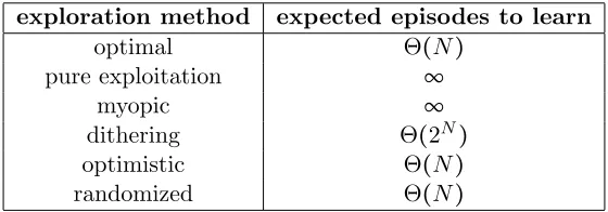
Table 1 summarizes our discussion of learning times of various exploration methods applied to Example 1. The minimal time required to learn an optimal policy, which is achieved by an agent who moves right whenever she knows how to, is Θ(N) episodes. The pure-exploitation algorithm avoidsanyactive exploration and requires Θ(2N)episodes to learn. Dithering does not help for our problem. Though more sophisticated, myopic approaches do not carry out deep exploration, and as such, still require Θ(2N) episodes. Optimistic and randomized approaches require only Θ(N) episodes.
exploration method expected episodes to learn
optimal Θ(N)
pure exploitation ∞
myopic ∞
dithering Θ(2N)
optimistic Θ(N)
randomized Θ(N)
Table 1: Expected number of episodes required to learn an optimal policy for Example 1.
5. Algorithms
the intention that this additional ingredient will broadly enable computationally efficient deep exploration.
Much of the literature and most notable applications build on value function learning. This involves fitting a parameterized value function to observed data in order to estimate the optimal value function. The algorithms we present will be of this genre. As a starting point, in Section 5.2, we will describe least-squares value iteration (LSVI), which is perhaps the simplest of value function learning algorithms. In Section 5.3, we consider modifying LSVI by injecting randomness in a manner that incentivizes deep exploration. This gives rise to a new class of algorithms, which we will refer to as randomized least-squares value iteration (RLSVI), and which offer computationally tractable means to deep exploration.
LSVI plays a foundational role in the sense that most popular value function learning algorithms can be interpreted as variations designed to improve computational efficiency or robustness to mis-specification of the parameterized value function. The reinforcement learning literature presents many ideas that address such practical considerations. In Sec-tion 5.4, we will discuss how such ideas can be brought to bear in tandem with RLSVI.
5.1. Value function learning
Before diving into specific reinforcement learning algorithms, let us discuss general concepts that apply to all of them. Value function learning algorithms make use of a family Q of state-action value functions indexed byθ∈Rd. EachQθ∶ S × A ↦Ridentifies a state-action value function.2 As a simple example of such a family, consider representing value functions as linear combinations of fixed features. In particular, if φ(s, a) ∈Rd is a vector of features designed to capture salient characteristics of the state-action pair (s, a), it is natural to consider the family of functions taking the formQθ(s, a) =θ⊺φ(s, a), withθ∈Rd.
Algorithm 1 (live) provides a template for reinforcement learning algorithms we will consider. It operates over an endless sequence of episodes, accumulating observations, learning value functions, and applying actions. We use a Pythonic pseudocode, with an object-oriented division into agentand environment. We use
transition=NamedTuple(old state,action,reward,new state,timestep),
to describe the evolution of the system. Where convenient, we will alternatively write
transition= (st, at, rt, s′t, t). We highlight three key methods theagent must implement:
• act– select actions given its internal value estimates, (e.g. greedy action selection). • update buffer– incorporate observations to its memory buffer, (e.g. append to list). • learn from buffer– update value estimate given the data in the buffer, (e.g. LSVI). The agents that we discuss will be distinguished through their implementation of these methods, which we will now outline.
The simplest form of act is given by the greedy strategy act greedy. An agent that uses this approach will select actions that maximize its estimated state-action value. If multiple actions attain the maximum, one is sampled uniformly from among them.3
2. We adopt notation that for allQ, parameterθ0=nullindicatesQθ0≡0.
Algorithm 1 live
Input: agent methodsact,update buffer,learn from buffer environment methodsreset,step
1: for`in (1,2, . . .)do
2: agent.learn from buffer()
3: transition ←environment.reset()
4: while transition.new state is notnull do
5: action←agent.act(transition.new state)
6: transition←environment.step(action)
7: agent.update buffer(transition)
Similarly, the simplest form of update buffer is to simply accumulate all observed data
update buffer queue. Our next two sections will investigate agents that store all observed data and take greedy actions; we investigate the effects of learn from bufferand explain why training least-squares value iteration on randomly perturbed versions of the data can offer a computationally tractable means to deep exploration.
5.2. Least-squares value iteration
Given an MDP M, one can apply the value iteration algorithm (Algorithm 2) to compute an arbitrarily close approximation toQ∗. The algorithm takesMand a planning horizonH as input and computesQ∗H, the optimal value over the next H time periods of the episode as a function of the current state and action. The computation is recursive: given Q∗h, the algorithm computes Q∗h+1 by taking the expected sum of immediate reward and Q∗h, evaluated at the next state, maximized over actions. Under Assumption 1, the mapping from Q∗h to Q∗h+1 is a weighted-maximum-norm contraction mapping (Bertsekas and Tsitsiklis, 1996), and as such, Q∗h converges to Q∗ at a geometric rate. Hence, for any M satisfying Assumption 1 and sufficiently largeH, the greedy policy with respect toQ∗H is optimal.
Algorithm 2 vi
Input: M = (S,A,R,P, ρ) MDP
H∈N planning horizon
Output: Q∗H optimal value function for H-period problem
1: Q∗0 ←0
2: forh in(0, . . . , H−1) do
3: Q∗h+1(s, a) ← ∑s′∈SPs,a(s′) (∫ rRs,a,s′(dr) +maxa′∈AQ∗
h(s′, a′)) ∀s, a∈ S × A
4: return Q∗H
(TD) loss:
(5.1) L(θ;θ−,D) ∶= ∑
t∈D
(rt+max
a′∈A
Qθ−(s′t, a′) − Qθ(st, at)) 2
.
Note that, ifQ spans the true value function Q∗ and the data Dmatches the distribution of M then the minimizer of L matches the solution of Algorithm 2; for more information see Sutton and Barto (2018).
Algorithm 3 (learn lsvi) describes the learn from buffer method for LSVI, whcih approximates the operations carried out by value iteration. The algorithm successively minimizes the empirical temporal difference loss (5.1) plus a regularization term:
(5.2) R(θ;θp) ∶= v
λ∥θ
p
−θ∥22.
Here θp can be interpreted as a prior for θ and vλ determines the strength of the regular-ization coefficient. In a linear system these correspond to a prior beliefθ∼N(θp, λI) with observationsyt=xtθ+ztforzt∼N(0, v). Similarly tovi,learn lsvicomputes a sequence of value functions(Qθh∶h=0, . . . , H), reflecting optimal expected rewards over an expand-ing horizon. However, while value iteration computes optimal values usexpand-ing full knowledge of the MDP, LSVI produces estimates based only on observed data. In each iteration, for each observed transition (s, a, r, s′), learn lsvi regresses the sum of immediate reward r and the value estimate maxa′∈AQθ˜
h(s
′, a′) at the next state onto the value estimateQ˜
θh+1(s, a)
for the current state-action pair.
Algorithm 3 learn lsvi
Agent: L(θ= ⋅;θ−= ⋅,D= ⋅ ) TD error loss function R(θ= ⋅;θp= ⋅ ) regularization function
buffer memory buffer of observations
prior prior distribution of θ
H∈N planning horizon
Updates: θ˜ agent value function estimate
1: θ˜0 ←null
2: Data ˜D ←buffer.data()
3: Prior parameter ˜θp ←prior.mean()
4: forh in(0, . . . , H−1) do
5: θ˜h+1←argmin
θ∈RD
(L(θ; ˜θh,D) + R(˜ θ; ˜θp))
6: update value function estimate ˜θ←θ˜H
In the event that the parameterized value function is flexible enough to represent every function mappingS × Ato R, it is easy to see that, for any θ and any positiveλand v, as the observed history grows to include an increasing number of transitions from each state-action pair, value functionsQθ˜
H produced by LSVI converge to Q
∗
H. However, in practical
contexts, the data set is finite and the parameterization is chosen to be less flexible in order to enable generalization. As such, Q˜
θH and Q
∗
In addition to inducing generalization, a less flexible parameterization is critical for computational tractability. In particular, the compute time and memory requirements of value iteration scale linearly with the number of states, which, due to the curse of dimen-sionality, grows intractably large in most practical contexts. LSVI sidesteps this scaling, instead requiring compute time and memory that scale polynomially with the dimension of the parameter vector ˜θ, the number of historical observations, and the time required to maximize over actions at any given state.
An LSVIagentmay also be paired with some dithering strategy for exploration, such as -greedy or Boltzmann exploration (4.2) in place ofact greedy. As discussed in Section 4, randomly perturbing greedy actions – or dithering – does not achieve deep exploration and so can lead to exponentially poor performance. Our next subsection introduces randomized value function estimates as an alternative.
5.3. Randomized least-squares value iteration
At a high level, the idea is to randomly sample an imagined optimal parameter ˜θaccording to the probability that it is optimal. This approach is inspired by Thompson sampling, an algorithm widely used in bandit learning (Thompson, 1933). In the context of a multi-armed bandit problem, Thompson sampling maintains a belief distribution over models that assign mean rewards to arms. As observations accumulate, this belief distribution evolves according to Bayes rule. When selecting an arm, the algorithm samples a model from this belief distribution and then selects the arm to which this model assigns largest mean reward. To address a reinforcement learning problem, one could in principle apply Thompson sampling to value function learning. This would involve maintaining a belief distribution over candidates for the optimal value function. Before each episode, we would sample a function from this distribution and then apply the associated greedy policy over the course of the episode. This approach could be effective if it were practically viable, but distributions over value functions are complex to represent and exact Bayesian inference would likely prove computationally intractable.
Randomized least-squares value iteration (RLSVI) is modeled after this Thompson sam-pling approach and serves as a computationally tractable method for samsam-pling value func-tions. RLSVI was first introduced in Wen (2014), and subsequent work has examined variations of RLSVI and their performance with both linear and nonlinear function approx-imation (Osband et al., 2016b,a; Osband, 2016). RLSVI does not explicitly maintain and update belief distributions and does not optimally synthesize information, as a coherent Bayesian method would. Regardless, as we will later establish through computational and mathematical analyses, RLSVI can offer an effective approach to deep exploration.
5.3.1. Randomization via Gaussian noise
We first consider a version of RLSVI that induces exploration through injecting Gaussian noise into calculations of the form carried out by LSVI. To understand the role of this noise, let us first consider a conventional linear regression problem. Suppose we wish to estimate a parameter vectorθ∈RD, with N(θ, λI) prior and dataD = ((xn, yn) ∶n=1, . . . , N), where each “feature vector” xn is a row vector with K components and each “target value” yn
according to yn =xnθ+wn, where wn is independently drawn from N(0, v). Conditioned on D,θis Gaussian with
(5.3) E[θ∣D] =argmin
θ∈RD
(1 v
N
∑
n=1
(yn−xnθ)2+1 λ∥θ−θ∥
2 ) = (1
vX ⊺X+1
λI) −1
(1 vX
⊺y+ 1 λθ)
and
Cov[θ∣D] = (1 vX
⊺X+1 λI)
−1 ,
whereX∈RN×D is a matrix whosenth row isxnandy∈Rnis a vector whosenth component isyn.
One way of generating a random sample ˜θ with the same conditional distribution as θ is simply to sample from ˜θ∼N(E[θ∣D],Cov[θ∣D]). An alternative construction is given by
(5.4) θ˜←argmin
θ∈RD
(1 v
N
∑
n=1
(yn+zn−xnθ)2+1 λ∥
ˆ
θ−θ∥2) = (1 vX
⊺X+1 λI)
−1 (1
vX
⊺(y+z) +1 λ ˆ θ),
where ˆθ∼N(θ, λI) and zn ∼N(0, v) are sampled independently. To see why this ˜θ takes on the same distribution, first note that ˜θis Gaussian, since it is affine inθand z. Further, ˜
θ exhibits the appropriate mean and covariance matrix, since
E[θ˜∣D] = ( 1 vX
⊺X+ 1 λI)
−1 (
1 vX
⊺(y+E[z∣D]) + 1 λE[
ˆ
θ∣D]) =E[θ∣D],
and
Cov[θ˜∣D] = (1 vX
⊺X+1 λI)
−1 (1
v2X ⊺
E[zz⊺∣D]X+ 1 λ2E[θˆθˆ
⊺∣D]) (1 vX
⊺X+1 λI)
−1
= (1 vX
⊺X+1 λI)
−1 (1
vX ⊺X+1
λI) ( 1 vX
⊺X+1 λI)
−1
= Cov[θ∣D].
Algorithm 4 learn rlsvi
Agent: L(θ= ⋅;θ−= ⋅,D= ⋅ ) TD error loss function R(θ= ⋅;θp= ⋅ ) regularization function
buffer memory buffer of observations
prior prior distribution of parameters
H∈N planning horizon
Updates: θ˜ agent value function estimate
1: θ˜0 ←null
2: Data ˜D ←buffer.sample perturbed data()
3: Prior parameter ˜θp ←prior.sample()
4: forh in(0, . . . , H−1) do
5: θ˜h+1←argmin
θ∈RD
(L(θ; ˜θh,D) + R(˜ θ; ˜θp))
6: update value function estimate ˜θ←θ˜H
Note thatlearn rlsviis identical tolearn lsviexcept that the optimization happens over randomized versions of the underlying data and prior. For correspondence with the Gaussian derivation above we would implement:
(5.5) buffer.sample perturbed data() ∶= [(st,at,rt+zt,s′t,t) ∀t∈buffer, zt∼N(0,v)].
We call this version of RLSVI with additive Gaussian noiselearn grlsvi, indicating the specific choice of data randomization and prior θ ∼N(0, λI). In Section 6 we prove that this method recovers a polynomial regret bound when used with linear value functions and tabular representation. This is significant, because LSVI with any dithering action selection scheme can not recover such a bound (Section 4). Before we jump to analysis, we provide some intuition for how this simple modification can lead to deep exploration.
5.3.2. How does RLSVI drive deep exploration?
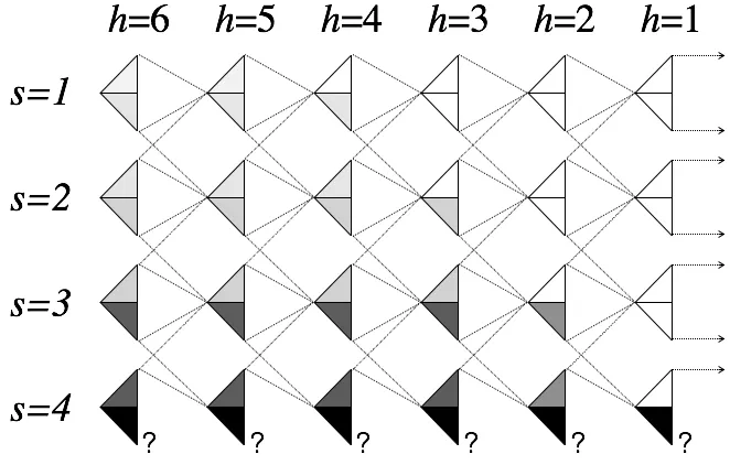
To understand the role of injected noise and how this gives rise to deep exploration, let us discuss a simple example, involving an MDP M with four states S = {1,2,3,4} and two actions A = {up,down}. Let H be a list of all transitions we have observed, and partition this into sublists Hs,a = ((s,˜ ˜a, r, s′) ∈ H ∶ (s,˜ ˜a) = (s, a)), each containing transitions from a distinct state-action pair. Suppose that ∣H(4,down)∣ = 1, while for each state-action pair (s, a) ≠ (4,down), ∣Hs,a∣ is virtually infinite. Hence, we are highly uncertain about the expected immediate rewards and transition probabilities at (4,down) but can infer these quantities with extreme precision for every other state-action pair.
Given our uncertainty about M,Q∗H for each planning horizonH is a random variable. Figure 2 illustrates our uncertainty in these values. Each larger triangle represents a pair
each smaller triangle represents our degree of uncertainty in the value of Q∗h(s, a). To be more concrete, take our measure of uncertainty to be the variance ofQ∗h(s, a).
Figure 2: Illustration of how learn grlsviachieves deep exploration.
For the case of h = 1, only immediate rewards influence Q∗1, and as such we are only uncertain aboutQ∗1(4,down). Stepping back toh=2, in addition to being highly uncertain about Q∗2(4,down), we are somewhat uncertain about Q∗2(4,up) and Q∗2(3,down), since these pairs can transition to (4,down) and be exposed to the uncertainty associated with that state-action pair. We are not as uncertain aboutQ∗2(4,up) andQ∗2(3,down) as we are about Q∗2(4,down) because from (4,up) and (3,down), there is reasonable chance that we will never see(4,down). Continuing to work our way leftward in the diagram, it is easy to visualize how uncertainty propagates as h increases.
Let us now turn our attention to the variance of samples Qθ˜
H(s, a) generated by learn grlsvi, which, for reasons we will explain, tend to grow and shrink with the vari-ance of Q∗H(s, a). To keep things simple, assume λ = ∞ and that we use an exhaustive – or “tabular” – representation of value functions. In particular, each component of the parameter vector θ∈R∣S∣×∣A∣ encodes the value Qθ(s, a) of a single state-action pair. This parameterized value function can represent any mapping fromS × A toR.
Under our simplifying assumptions, it is easy to show that
Q˜
θh+1(s, a) =
1
∣H˜s,a∣
∑ (˜s,˜a,r,s′,z)∈H˜
s,a
(r+max
a′∈A
Q˜
θh(s
′, a′) +z).
The right-hand-side is an average of target values. Recall that, for any (s, a) ≠ (4,down), ∣H˜s,a∣is so large that any sample average is extremely accurate, and therefore,Q˜
θh+1(s, a)is
essentially equal toEM[rt+1+maxα∈AQθ˜
h(st+1, α)∣st=s, at=a]. For the distinguished case
of (4,down), ∣H˜4,down∣ =1, and the average target value may therefore differ substantially from its expectation E[r+maxa′∈AQ˜
θh(s
average out as it does for other state-action pairs and should contribute variancev to the sample Qθ˜
h+1(4,down).
Based on this observation, for the case of h = 1, for (s, a) ≠ (4,down), Qθ1˜ (s, a) is virtually equal to Q∗1, while for Qθ1˜ (4,down) exhibits variance of at least v. For h = 2, Q˜
θ2(4,down) again exhibits variance of at leastv, but unlike the case ofh =1, Qθ2˜ (4,up)
and Qθ2˜ (3,down) also exhibit non-negligible variance since these pairs can transition to (4,down)and therefore depend on the noise-corrupted realization ofQθ1˜ (4,down). Working leftward through Figure 2, we can see that noise propagates and influences value estimates in a manner captured by the shading in the figure. Hence, samples Q˜
θh(s, a) exhibit high
variance where the variance ofQ∗h(s, a) is large.
This relationship drives deep exploration. In particular, a high variance sampleQ˜
θH(s, a)
will be overly optimistic in some episodes. Over such episodes, the agent will be incentivized to try the associated action. This is appropriate because the agent is uncertain about the optimal valueQ∗H(s, a)over the planning horizon. Note that this incentive is not only driven by uncertainty concerning the immediate reward and transition. As illustrated in Figure 2, uncertainty propagates to offer incentives for the agent to pursue information even if it will require multiple time periods to arrive at an informative observation. This is the essence of deep exploration.
It is worth commenting on a couple subtle properties of learn grlsvi. First, given θh and H, θh+1 is sampled from a Gaussian distribution. However, given the inputs to
learn grslvi, the output ˜θ is not Gaussian. This is because at each step θh+1 depends nonlinearly on θh due to the maximization over actions in the TD loss (5.1). Second, it
is important that learn grlsvi uses the same noise samples z in across iterations of the for loop in line 5. To see why, suppose learn grlsvi used independent noise samples in each iteration. Then, when applied to the example of Figure 2, in some iterations, we would be optimistic about the reward at (4,down), while in other iterations, we would be pessimistic about that. Now consider a sample Qθ˜
H(1,up) for large H. This sample
would be perturbed by a combination of optimistic and pessimistic noise terms influencing assessments at(4,down)to the right. The resulting averaging effect could erode the chances thatQθ˜
H(1,up) is optimistic.
5.3.3. Randomization via statistical bootstrap
With learn grlsvi, the Gaussian distribution of noise serves as a coarse model of errors between targets r+maxa′∈AQ˜
θh(s
′, a′) and expectations E[r+max
a′∈AQ˜
θh(s
′, a′)∣θ˜h,M].
The statistical bootstrap4 offers an alternative approach to randomization which may often more accurately capture characteristics of the generating process. In its classic form, the bootstrap takes a dataset D of size N and generates a sampled dataset ˜D also of size N drawn uniformly with replacement from D (Efron and Tibshirani, 1994). The bootstrap serves as a form of data-based simulation and, in certain cases, recovers strong convergence guarantees (Bickel and Freedman, 1981; Fushiki, 2005).
learn brlsviis a version of RLSVI that makes use of the bootstrap in place of additive Gaussian noise. This algorithm followslearn rlsvi (Algorithm 4) and implements
(5.6) buffer.sample perturbed data() ∶=bootstrap sample(buffer.data()).
Bootstrap sampling for value function randomization may present several benefits over additive Gaussian noise. First, most bootstrap resampling schemes do not require a ‘noise variance’ as input, which simplifies the algorithm from a user perspective. Related to this point, the bootstrap can effectively induce a state-dependent and heteroskedastic random-ization which may be more appropriate in complex environments. More generally, we can consider bootstrapped RLSVI as a non-parameteric randomization for the value function estimate and this opens a wide range of potential bootstrap variants and prior mechanisms that could be employed with RLSVI (Osband and Van Roy, 2015).
Eckles and Kaptein (2019) were the first to propose using bootstrap samples as an approximation to the posterior samples used in the Thompson sampling algorithm. Unfor-tunately, bootstrapping does not provide meaningful uncertainty estimates in early periods. If applied without modification, the algorithms in Eckles and Kaptein (2019) incur regret that scales linearly in the time horizon. Value function estimates in learn brlsvi are in-stead randomized not just through bootstrap sampling, but through regularizing toward a random prior sample. The effect of the random prior sample vanishes as diverse data is collected, but it is critical to driving exploration in early periods.
5.4. Practical variants of RLSVI
In this section, we will present variants of RLSVI designed to address the important prac-tical considerations of computational efficiency and robustness to mis-specification of the parameterized value function. There are many ideas in the reinforcement learning literature that can be brought to bear for these purposes, and we will by no means cover an exhaustive list. Rather, we will present a mix of ideas that lead to a particular algorithm that effec-tively addresses a broad range of complex problems. This algorithm also serves to illustrate the many degrees of freedom in mixing and matching ingredients from the reinforcement learning literature when randomized value functions are part of the recipe.
5.4.1. Finite buffer experience replay
The use of a buffer of past observations to fit a value function is sometimes referred to as experience replay. The algorithms we have presented so far use an infinite buffer and thus require memory and compute time that grow linearly in the number of observations. For complex problems that require substantial learning times, such a requirement becomes onerous. To overcome this, we can restrict the buffer to some finite size, treating it as a FIFO queue.
here. Recent work has also demonstrated benefit from more sophisticated prioritization of data for storage in a finite buffer (Schaul et al., 2015).
5.4.2. Discounted TD and incremental learning
Both LSVI and RLSVI take a planning horizonH∈Nas an argument. These approaches can be wasteful in that they compute separate estimates ˜θh for each h=1, .., H. Further, these algorithms are “batch,” in the sense that they require computation over all observed data at the start of each episode; this leads to computational costs that grow with time. In this subsection we introduce a discounted formulation that admits an incremental computational approach.
Let γ ∈ (0,1) be a discount factor that induces a time preference over future rewards. A discountγ approximates an effective planning horizon H≃ 1
1−γ, but affords a solution to
the discounted Bellman equation Q∗γ(s, a) = EM[R(s, a) +γmaxa′Q∗γ(s′, a′)] (Blackwell,
1965). Inspired by this relationship we define the γ-discounted empirical TD loss:
(5.7) Lγ(θ;θ−,D) ∶= ∑
t∈D
(rt+γmax
a′∈A
Qθ−(s′t, a′) − Qθ(st, at))
2 .
Algorithm 5 (learn online lsvi) presents an incremental variant of LSVI. Rather than recompute ˜θ from scratch each episode, learn online lsviupdates its previous estimate by gradient descent over a subset of the data. This algorithm is a form of temporal differ-ence learning (Sutton, 1988) and, at a high level, this approach broadly describes famous approaches such as TD-gammon (Tesauro, 1995) and DQN (Mnih et al., 2015). For more background and discussion of this family of algorithms we refer to Sutton and Barto (2018).
Algorithm 5 learn online lsvi
Agent: θ˜ parameter estimate
˜
θp prior mean of parameter estimate
Lγ(θ= ⋅;θ−= ⋅,D= ⋅ ) TD error loss function R(θ= ⋅;θp= ⋅ ) regularization function
buffer memory buffer of observations
α learning rate
Updates: θ˜ agent value function estimate
1: Data ˜D ←buffer.sample minibatch()
2: δ←buffer.minibatch size/buffer.size
3: θ˜←θ˜−α∇
θ∣θ=θ˜(Lγ(θ; ˜θ,D) +˜ δR(θ; ˜θ p))
5.4.3. Randomization via ensemble sampling
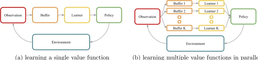
Ensemble sampling approximates the distribution induced by RLSVI through an en-semble of K ∈N estimates trained in parallel (θ1, ..,˜ θ˜K) (Osband and Van Roy, 2015; Lu and Van Roy, 2017). At the start of any episodel, we can approximate the distribution of ˜
θunder RLSVI via a sample of ˜θkfork∼Unif(1, .., K). Figure 3 presents an illustration of such a system.
(a) learning a single value function (b) learning multiple value functions in parallel
Figure 3: RLSVI via ensemble sampling, each member produced by LSVI on perturbed data.
One method to maintain K estimates in parallel is to implement an ensemble mem-ory buffer ensemble buffer. An ensemble buffer should function similarly to buffer, but maintain K distinct perturbations of the observed data ˜Dk, each associated with their ap-propriate ensemble value estimate ˜θk. We use a Pythonic notation thatensemble buffer[k] is abufferfor eachk=1, ..,K; although in a practical implementation it will be sensible to share appropriate parts of the memory requirements. For an online variant oflearn grlsvi
(additive Gaussian noise) we can store K distinct samples of additive noise, as described in Algorithm 6. Similarly, for an online approximation to bootstrap sampling we might use “double-or-nothing” sampling per Algorithm 7 (Owen and Eckles, 2012).
Algorithm 8 (learn ensemble rlsvi) presents the ensemble RLSVI algorithm. An agent that employslearn ensemble rlsvimaintains ensemble parameter estimates ˜θ1, ..,θ˜K
with random prior samples ˜θ1p, ..,θ˜Kp . The regulatization effects of R(θ; ˜θpk) can play an im-portant role in exploration. Although we have suggested a particular form in (5.2), we would consider alternative approaches based on prior observations as studied in off-policy learning (Precup et al., 2001) andtransfer learning (Taylor and Stone, 2009).
We note that, when used off-policy, minimizing the TD loss may lead to unstable learning and even cause the value function estimate to diverge (Tsitsiklis and Van Roy, 1997). This instability can be exacerbated by algorithms such as learn ensemble rlsvi, which may lead to value estimates computed from data more off-policy than a single value estimate. In this context, it may be beneficial to replace the naive TD loss with an alternative designed for off-policy learning (Sutton et al., 2009; Munos et al., 2016).
Algorithm 6 ensemble buffer.update gaussian noise(⋅) Input: transition (st, at, rt, s′t, t)
Agent: v noise variance
Updates: ensemble buffer replay buffer ofK-parallel perturbed data
1: fork in(1, . . . , K) do
Algorithm 7 ensemble buffer.update bootstrap(⋅) Input: transition (st, at, rt, s′t, t)
Updates: ensemble buffer replay buffer ofK-parallel perturbed data
1: fork in(1, . . . , K) do
2: if mkt ∼Unif({0,1}) =1 then
3: ensemble buffer[k].enqueue((st, at, rt, s′t, t))
Algorithm 8 learn ensemble rlsvi
Agent: θ˜1, ..,θ˜K ensemble parameter estimates
˜
θ1p, ..,θ˜pK prior samples of parameter estimates Lγ(θ= ⋅;θ−= ⋅,D= ⋅ ) TD error loss function
R(θ= ⋅;θp= ⋅ ) regularization function
ensemble buffer replay buffer of K-parallel perturbed data
α Learning rate
Updates: θ˜ agent value function estimate
1: fork in(1, . . . , K) do
2: Data ˜Dk←ensemble buffer[k].sample minibatch()
3: δ←buffer.minibatch size/buffer.size
4: θ˜k←θ˜k−α∇θ∣θ=θ˜
k(Lγ(θ; ˜θk,
˜
Dk) + R(θ; ˜θpk))
5: update ˜θ←θ˜j forj∼Unif(1, .., K)
6. Regret bound
This section provides a regret analysis of RLSVI in a particularly simple type of decision problem (Section 3). We consider an RLSVIagent with an infinite buffer, greedy actions and learn grlsvi (Algorithm 4 with additive Gaussian noise (5.5)) and a tabular repre-sentation.5 The bound we establish applies to a tabular time-inhomogeneous MDP with transition kernel drawn from a Dirichlet prior. This stylized setting provides rigorous confir-mation that RLSVI is capable of performing provably efficient deep exploration in tabular environments. In addition, we hope this analysis provides a framework for establishing more general guarantees – for example those applying to RLSVI with linearly parameter-ized value functions. Several intermediate lemmas used in the analysis hold under much less restrictive assumptions, and could be useful beyond the setting studied here.
6.1. Formulation of a time-inhomogenous MDP
We consider a class offinite-horizon time-inhomogeneous MDPs. This can be formulated as a special case the paper’s general formulation as follows. Assume the state space factorizes as S = S0∪ S1∪ S2∪ ⋯ ∪ SH−1 where the state always advances from some state st ∈ St to st+1 ∈ St+1 and the process terminates with probability 1 in period H. For notational convenience, we assume each set S0, ...,SH−1 contains an equal number of elements. This
is stated formally in the next assumption, which is maintained for all statements in this section.
Assumption 2 (Finite-horizon time-inhomogeneous MDP)
The state space factorizes as S = S0∪ S1∪ S2∪ ⋯ ∪ SH−1 where ∣S0∣ = ⋯ = ∣SH−1∣ < ∞. For
any MDP M = (S,A,R,P, ρ),
∑
s′∈S t+1
Ps,a(s′) =1 ∀t∈ {0, ..., H−2}, s∈ St, a∈ A,
and
∑
s′∈S
Ps,a(s′) =0 ∀s∈ SH−1, a∈ A.
Each state s∈ St can be written as a pairs= (t, x) wheret∈ {0, ..., H−1} and x∈ X =
{1, ...,∣S0∣}. Similarly, a policy π ∶ S → A can be viewed as a sequence π = (π0, ..., πH−1) where πt∶x↦π((t, x)). Our notation can be specialized to this time-inhomogenous prob-lem, writing transition probabilities asPt,x,a(x′) ≡ P(t,x),a((t+1, x′))and reward probabil-ities as Rt,x,a,x′(r) ≡ R(t,x),a,(t+1,x′)(r). For consistency, we also use different notation for
the optimal value function, writing
VMπ,t(x) ≡VMπ((t, x))
and defineVM∗,t(x) ∶=maxπVMπ,t(x). Similarly, we can define the state-action value function under the MDP at timestept∈ {0, ..., H−1}by
Q∗M,t(x, a) =E[rt+1+VM∗,t+1(xt+1) ∣ M, xt=x, at=a] ∀x∈ X, a∈ A.
This is the expected reward accrued by taking actionain statexand proceeding optimally thereafter.
Upon choosing an action, the algorithm observes a pair o= (x′, r) consisting of a state transition and a reward. We will refer to this pairoas anoutcome of the decision. Assump-tions about the distribution of rewards and state-transiAssump-tions can be more compactly written as an assumption about outcome distributions. We study the regret of RLSVI under the following Bayesian model for the MDPM. This assumption is not required for some of the results in this section, and we will specify when it is needed.
Assumption 3 (Independent Dirichlet prior for outcomes)
Rewards take values in{0,1}and so the cardinality of the outcome space is∣X ×{0,1}∣ =2∣X ∣.
For each,(t, x, a) ∈ {0, ..., H−2} × X × A, the outcome distribution is drawn from a Dirichlet
prior
Pt,x,aO (⋅) ∼Dirichlet(α0,t,x,a)