Sharp Oracle Inequalities for Square Root Regularization
Benjamin Stucky [email protected]
Seminar for Statistics ETH Z¨urich
R¨amistrasse 101
8092 Zurich, Switzerland
Sara van de Geer [email protected]
Seminar for Statistics ETH Z¨urich
R¨amistrasse 101
8092 Zurich, Switzerland
Editor:Nicolas Vayatis
Abstract
We study a set of regularization methods for high-dimensional linear regression models. These penalized estimators have the square root of the residual sum of squared errors as loss function, and any weakly decomposable norm as penalty function. This fit measure is chosen because of its property that the estimator does not depend on the unknown standard deviation of the noise. On the other hand, a generalized weakly decomposable norm penalty is very useful in being able to deal with different underlying sparsity structures. We can choose a different sparsity inducing norm depending on how we want to interpret the unknown parameter vector β. Structured sparsity norms, as defined in Micchelli et al. (2010), are special cases of weakly decomposable norms, therefore we also include the square root LASSO (Belloni et al., 2011), the group square root LASSO (Bunea et al., 2014) and a new method called the square root SLOPE (in a similar fashion to the SLOPE from Bogdan et al. 2015). For this collection of estimators our results provide sharp oracle inequalities with the Karush-Kuhn-Tucker conditions. We discuss some examples of estimators. Based on a simulation we illustrate some advantages of the square root SLOPE.
Keywords: Square root LASSO, structured sparsity, Karush-Kuhn-Tucker, sharp oracale inequality, weak decomposability
1. Introduction and Model
The recent development of new technologies makes data gathering not a big problem any more. In some sense there is more data than we can handle, or than we need. The problem has shifted towards finding useful and meaningful information in the big sea of data. An example where such problems arise is the high-dimensional linear regression model
Y =Xβ0+. (1.1)
HereY is then−dimensional response variable,Xis then×pdesign matrix andis the iden-tical and independent distributed noise vector. The noise has E(i) = 0,Var(i) =σ2, ∀i∈
{1, ..., n}. Assume thatσ isunknown, and thatβ0 is the ”true” underlyingp−dimensional
c
parameter vector of the linear regression model with active setS0 := supp(β0).
While trying to explainY through different other variables, in the high-dimensional linear regression model, we need to set less important explanatory variables to zero. Otherwise we would have overfitting. This is the process of finding a trade-off between a good fit and a sparse solution. In other words we are trying to find a solution that explains our data well, but at the same time only uses more important variables to do so.
The most famous and widely used estimator for the high-dimensional regression model is the`1−regularized version of least squares, called LASSO (Tibshirani, 1996)
ˆ
βL(σ) := arg min β∈Rp
kY −Xβk2n+ 2λ1σkβk1 .
Hereλ1 is a constant called the regularization level, which regulates how sparse our solution should be. Also note that the construction of the LASSO estimator depends on the unknown noise level σ. We moreover let kak1 := Ppi=1|ai|for any a∈ Rp denote the `1−norm and for anya∈Rn we write kak2
n=
Pn
j=1a2j/n, the `2−norm squared and divided by n. The LASSO uses the`1−norm as a measure of sparsity. This measure as regulizer sets a number of parameters to zero.
Let us rewrite the LASSO into the following form
ˆ
βL= arg min β∈Rp
kY −Xβkn+λ
0
(β)kβk1
· 2λ1σ
λ0(β)
,
where λ0(β) := 2λ1σ
kY−Xβkn.Instead of minimizing with λ
0
(β), a function ofβ, let us assume
that we keep λ0(β) a fixed constant. Then we get the Square Root LASSO method
ˆ
βsrL:= arg min β∈Rp
{kY −Xβkn+λkβk1}.
So in some sense theλfor the Square Root LASSO is a scaled version, scaled by an adaptive estimator ofσ, of λ1 from the LASSO. By the optimality conditions it is true that
ˆ
βL(kY −XβˆsrLkn) = ˆβsrL.
The idea of the square root LASSO was further developed in Bunea et al. (2014) to the group square root LASSO, in order to get a selection of groups of predictors. The group LASSO norm is another way to describe an underlying sparsity, namely if groups of parameters should be set to zero, instead of individual parameters. Another extension for the the square root LASSO in the case of matrix completion was given by Klopp (2014).
Now in this paper we go further and generalize the idea of the square root LASSO to any sparsity inducing norm. From now on we will look at the family of norm penalty regularization methods, which are of the following square root type
ˆ
β:= arg min
β∈Rp
{kY −Xβkn+λΩ(β)},
where Ω is any norm on Rp. This set of regularization methods will be called square root regularization methods. Furthermore, we introduce the following notations
ˆ
:=Y −Xβˆ the residuals, Ω∗(x) := max
z,Ω(z)≤1z
Tx, x∈
Rp the dual norm of the norm Ω, and
βS ={βj :j∈S} ∀S⊂ {1, ..., p} and all vectorsβ ∈Rp.
Later we will see that describing the underlying sparsity with an appropriate sparsity norm can make a difference in how good the errors will be. Therefore in this paper we extend the idea of the square root LASSO with the`1−penalty to more general weakly decomposable norm penalties. The theoretical λ of such an estimator will not depend on σ either. We introduce the Karush-Kuhn-Tucker conditions for these estimators and give sharp oracle inequalities. In the last two sections we will give some examples of different norms and simulations comparing the square root LASSO with the square root SLOPE.
2. Karush-Kuhn-Tucker Conditions
As we already have seen before, these estimators need to calculate a minimum overβ. The Karush-Kuhn-Tucker conditions characterize this minimum. In order to formulate these optimality conditions we need some concepts of convex optimization. For the reader who is not familiar with this topic, we will introduce the subdifferential, which generalizes the differential, and give a short overview of some properties, as can be found for example in Bach et al. (2012). For any convex functiong :Rp → R and any vector w ∈Rp we define its subdifferential as
∂g(w) :={z∈Rp; g(w0)≥g(w) +zT(w0−w) ∀w0 ∈Rp}.
The elements of∂g(w) are called the subgradients ofg atw.
Let us remark that all convex functions have non empty subdifferentials at every point. Moreover by the definition of the subdifferential any subgradient defines a tangent space
w0 7→g(w)+zT·(w0−w), that goes throughg(w) and is at any point lower than the function
next lemma, which dates back to Pierre Fermat (see Bauschke and Combettes 2011), shows how to find a global minimum for a convex functiong.
Lemma 1 (Fermat’s Rule) For all convex functions g:Rp →R it holds that
v∈Rp is a global minimum of g ⇔0∈∂g(v).
For any norm Ω onRp withω ∈Rp it holds true that its subdifferential can be written as (see Bach et al. 2012 Proposition 1.2)
∂Ω(ω) =
(
{z∈Rp; Ω∗(z)≤1} ifω= 0 {z∈Rp; Ω∗(z) = 1VzTw= Ω(ω)} ifω6= 0.
(2.1)
We are able to apply these properties to our estimator ˆβ. Lemma 1 implies that
ˆ
β is optimal ⇔ −1
λ∇kY −X
ˆ
βkn∈∂Ω( ˆβ).
This means that, in the case kˆkn > 0, for the square root regularization estimator ˆβ it
holds true that
ˆ
β is optimal ⇔ X
T(Y −Xβˆ)
nλkY −Xβˆkn ∈∂Ω( ˆβ). (2.2) By combining equation (2.1) with (2.2) we can write the KKT conditions as
ˆ
β is optimal ⇔
Ω∗nˆkTˆXk
n
≤λ if ˆβ = 0
Ω∗
ˆ
TX nkˆkn
=λ if ˆβ 6= 0.
VˆTXβˆ
nkˆkn =λΩ( ˆβ)
(2.3)
What we might first remark about equation (2.3) is that in the case of ˆβ 6= 0 the second part can be written as
ˆ
TXβ/nˆ = Ω( ˆβ)·Ω∗
ˆ
TX n
.
This means that we in fact have equality in the generalized Cauchy-Schwartz Inequality for these two p−dimensional vectors. Furthermore let us remark that the equality
ˆ
TXβ/nˆ = Ω( ˆβ)λkˆkn
trivially holds true for the case where ˆβ = 0. It is important to remark here that, in contrast to the KKT conditions for the LASSO, we have an additionalkˆkn term in the expression
Ω∗nˆkTˆXk
n
. This nice scaling leads to the property that the theoreticalλis independent of
σ.
With the KKT conditions we are able to formulate a generalized type of KKT conditions. This next lemma is needed for the proofs in the next chapter.
Lemma 2 For the square root type estimator βˆwe have for anyβ ∈Rp and when kˆk n6= 0
1 kˆknˆ
Proof First we need to look at the inequality from the KKT’s, which holds in any case
Ω∗
ˆ
TX nkˆkn
≤λ. (2.4)
And by the definition of the dual norm and the maximum, we have with (2.4)
1 kˆknˆ
TXβ/n≤Ω(β)· max β∈Rp,Ω(β)≤1
ˆ
T
kˆknXβ/n
= Ω(β)·Ω∗
ˆ
TX
nkˆkn
≤Ω(β)λ. (2.5)
The second equation from the KKT’s, which again holds in any case, is
1 kˆknˆ
TXβ/nˆ =λΩ( ˆβ). (2.6)
Now putting (2.5) and (2.6) together we get the result.
3. Sharp Oracle Inequalities for the square root regularization estimators
We provide sharp oracle inequalities for the estimator ˆβ with a norm Ω that satisfies a so called weak decomposability condition. An oracle inequality is a bound on the estimation and prediction errors. This shows how good these estimators are in estimating the parame-ter vectorβ0. This is an extension of the sharp oracle results given in van de Geer (2014) for LASSO type of estimators, which in turn was an generalization of the sharp oracle inequal-ities for the LASSO and nuclear norm penalization in Koltchinskii (2011) and Koltchinskii et al. (2011).
3.1 Concepts and Assumptions
Let us first introduce all the necessary definitions and concepts. Some normed versions of values need to be introduced:
f = λΩ(β 0) kkn
λSc = Ω
Sc∗
((TX)Sc)
nkkn
λS = Ω
∗((TX) S)
nkkn
λm = max(λS, λSc)
λ0 = Ω
∗(TX)
nkkn
For example the quantity f gives the measure of the true underlying normalized sparsity. ΩSc denotes a norm onRp−|S|which will shortly be defined in Assumption II. Furthermore
λm will take the role of the theoretical (unknown) λ. If we compare this to the case of the LASSO we see that instead of the `∞−norm we generalized it to the dual norm of
Ω. Also remark that in λm a term k1k
n appears. This scaling is due to the square root
regularization, which will be the reason thatλcan be chosen independently of the unknown standard deviation σ. Now we will give the two main assumptions that need to hold in order to prove the oracle inequalities. Assumption I deals with avoiding overfitting, and the main concern of Assumption II is that the norm has the desired property of promoting a structured sparse solution ˆβ. We will later see, that the structured sparsity norms in Micchelli et al. (2010) and Micchelli et al. (2013) are all of this form. Thus, Assumption II is quite general.
3.1.1 Assumption I (overfitting)
If kˆkn = 0, then ˆβ does the same thing as the Ordinary Least Squares (OLS) estimator
βOLS, namely it overfits. That is why we need a lower bound onkˆkn. In order to achieve
this lower bound we make the following assumptions:
P Y ∈ {Ye : min
β,s.t.Xβ=Ye
Ω(β)≤ kkn} !
= 0.
λ0
λ 1 + 2f
<1.
The λλ0 term makes sure that we introduce enough sparsity (no overfitting).
3.1.2 Assumption II (weak decomposability)
Assumption II is fulfilled for a setS ⊂ {1, ..., p}and a norm Ω on Rp if this norm is weakly decomposable, andS is an allowed set for this norm. This was used by van de Geer (2014) and goes back to Bach et al. (2012). It is an assumption on the structure of the sparsity inducing norm. By the triangle inequality we have:
Ω(βSc)≥Ω(β)−Ω(βS).
But we will also need to lower bound this by another norm evaluated at βSc. This is
motivated by relaxing the following decomposability property of the`1-norm: kβk1=kβSk1+kβSck1,∀ setsS⊂1, ..., p and allβ ∈Rp.
This decomposability property is used to get oracle inequalities for the LASSO. But we can relax this property, and introduce weakly decomposable norms.
Definition 3 (Weak decomposability) A norm Ω in Rp is called weakly decomposable
for an index set S⊂ {1, ..., p}, if there exists a norm ΩSc on
R|S
c|
such that
∀β ∈Rp Ω(β)≥Ω(βS) + ΩS c
Furthermore we call a setS allowed if Ω is a weakly decomposable norm for this set.
Remark 4 In order to get a good oracle bound, we will choose the norm ΩSc as large as possible. We will also choose the allowed sets S in such a way to reflect the active set S0.
Otherwise we would of course be able to choose as a trivial example the empty set S=∅.
Now that we have introduced the two main assumptions, we can introduce other definitions and concepts also used in van de Geer (2014).
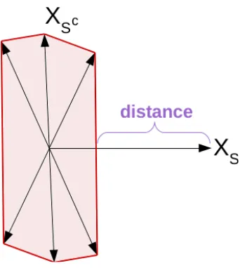
Definition 5 ForSan allowed set of a weakly decomposable normΩ, andL >0a constant, the Ω−eigenvalue is defined as
δΩ(L, S) := min
kXβS−XβSckn: Ω(βS) = 1,ΩS c
(βSc)≤L .
Then the Ω−effective sparsity is defined as
Γ2Ω(L, S) := 1
δ2Ω(L, S).
The Ω−eigenvalue is the distance between the two sets (van de Geer and Lederer, 2013) {XβS : Ω(βS) = 1} and {XβSc : ΩS
c
(βSc) ≤ L}, see Figure 2. The additional discussion
about these definitions will follow after the main theorem. The Ω−eigenvalue generalizes the compatibility constant (van de Geer, 2007).
For the proof of the main theorem we need some small lemmas. For any vector β ∈ Rp the (L, S)−cone condition for a norm Ω is satisfied if ΩSc(βSc) ≤ LΩ(βS), with L > 0 a
constant and S an allowed set.
The proof of Lemma 6 can be found in van de Geer (2014). It shows the connection between the (L, S)−cone condition and the Ω−eigenvalue. We bound Ω(βS) by a multiple ofkXβkn.
Lemma 6 Let S be an allowed set of a weakly decomposable normΩandL >0a constant. Then we have that the Ω−eigenvalue is of the following form:
δΩ(L, S) = min
kXβkn
Ω(βS)
, β satisfies the cone condition and βS 6= 0
.
We haveΩ(βS)≤ΓΩ(L, S)kXβkn.
We will also need a lower and an upper bound forkˆkn, as already mentioned in Assumption
I. The next Lemma 7 gives such bounds.
Lemma 7 Suppose that Assumption I holds true. Then
1 +f ≥ kˆkn kkn
≥ 1−
λ0
λ(1 + 2f)
f+ 2 >0.
Proof The upper bound is obtained by the definition of the estimator
Therefore we get
kˆkn≤ kkn+λΩ(β0).
Dividing bykknand by the definition off we get the desired upper bound. The main idea
for the lower bound is to use the triangle inequality
kˆkn=k−X( ˆβ−β0)kn≥ kkn− kX( ˆβ−β0)kn,
and then upper boundkX( ˆβ−β0)k
n. With Lemma 2 we get an upper bound for kX( ˆβ−
β0)kn,
kX( ˆβ−β0)k2n≤TX( ˆβ−β0)/n+λkˆkn(Ω(β0)−Ω( ˆβ))
≤λ0kknΩ( ˆβ−β0) +λkˆkn(Ω(β0)−Ω( ˆβ)) ≤λ0kkn(Ω( ˆβ) + Ω(β0)) +λkˆkn(Ω(β0)−Ω( ˆβ))
≤λ0kknΩ( ˆβ) + Ω(β0)(λ0kkn+λkˆkn).
In the second line we used the definition of the dual norm, and the Cauchy-Schwartz in-equality. Again by the definition of the estimator we have
Ω( ˆβ)≤ kkn
λ + Ω(β
0). And we are left with
kX( ˆβ−β0)kn≤ kkn s
λ0
λ
1 + 2λΩ(β 0) kkn
+ λ
λ0 · kˆkn kkn
·λΩ(β 0) kkn
.
By the definition off we get
kX( ˆβ−β0)kn≤ kkn s
λ0
λ
1 + 2f+ λ
λ0 kˆkn kkn
f
.
=kkn
s
λ0
λ + 2 λ0
λf+
kˆkn
kknf .
Now we get
kˆkn≥ kkn− kX( ˆβ−β0)kn
≥ kkn− kkn
s
λ0
λ + 2 λ0
λf +
kˆkn
kkn
f (3.1)
Let us rearrange equation (3.1) further in the case kˆkn
kkn <1
λ0 λ + 2
λ0 λf+
kˆkn
kkn
f ≥
1−kˆkn kkn
2
kˆkn
kknf ≥1−2 kˆkn
kkn + kˆk2
n
kk2
n
−λ 0
kˆkn
kkn
f + 2kˆkn kkn
≥1−λ 0
λ(1 + 2f)
kˆkn kkn ≥
1−λ0
λ(1 + 2f)
f+ 2
Assumption I
> 0.
On the other hand if kˆkn
kkn >1, we already get a lower bound which is bigger than
1−λ0 λ(1+2f)
f+2 .
3.2 Sharp Oracle Inequality
Finally we are able to present the main theorem. This theorem gives sharp oracle inequalities on the prediction error expressed in the`2-norm, and the estimation error expressed in the Ω and ΩSc norms.
Remark 8 Let us first briefly remark that in the Theorem 9 we need to assure that λ∗−
λm>0. The assumption λλm <1/a, with achosen as in Theorem 9, together with the fact thatλ0 ≤λm leads to the desired inequality
λ∗
λ =
1−λλ0(1 + 2f)
f + 2 ≥
1−λλm(1 + 2f)
f + 2 >
λm λ .
Theorem 9 Assume that0≤δ <1, and also thataλm < λ, with the constanta= 3(1+f). We invoke also Assumption I (overfitting) and Assumption II (weak decomposability) forS
and Ω. Here the allowed setS is chosen such that the active set Sβ := supp(β) is a subset of S. Then it holds true that
kX( ˆβ−β0)k2n+ 2δkkn
h
(λ∗+λm)Ω( ˆβS−β) + (λ∗−λm)ΩS c
( ˆβSc)
i
≤ kX(β−β0)k2n+kk2nh(1 +δ)(˜λ+λm)i2Γ2Ω(LS, S), (3.2)
with LS:=
˜
λ+λm
λ∗−λm1+1−δδ and
λ∗ :=λ 1−
λ0
λ(1 + 2f)
f+ 2
!
, λ˜ :=λ(1 +f).
Furthermore we get the two oracle inequalities
kX( ˆβ−β0)k2n≤ kX(β?−β0)k2n+kk2n(1 +δ)2(˜λ+λS c ?)2·Γ2
Ω(LS?, S?)
Ω( ˆβS?−β?) + ΩS c ?( ˆβ
Sc ?)≤
1 2δkkn
·kX(β?−β 0)k2
n
λ∗−λm +...
+(1 +δ) 2kk
n
2δ ·
(˜λ+λm)2
λ∗−λm ·Γ
2
For all fixed allowed sets S define
β?(S) := arg min β: supp(β)⊆S
kX(β−β0)k2n+kk2nh(1 +δ)(˜λ+λm)
i2
Γ2Ω(LS, S)
.
Then S? is defined as
S? := arg min Sallowed
kX(β?(S)−β0)k2n+kk2n
h
(1 +δ)(˜λ+λm)
i2
Γ2Ω(LS, S)
, (3.3)
β? :=β?(S?) (3.4)
it attains the minimal right hand side of the oracle inequality (3.2). An improtant special case of equation (3.2) is to choose β ≡β0 with S ⊇S0 allowed. The term kX(β−β0)k2n vanishes in this case and only the Ω−effective sparsity term remains for the upper bound. But it is not obvious in which cases and whether β? leads to a substantially lower bound than β0.
Proof Let β ∈Rp and letS be an allowed set containing the active set of β. We need to
distinguish 2 cases. The second case is the more substantial one. Case 1: Assume that
hX( ˆβ−β0), X( ˆβ−β)in≤ −δkknh(λ∗+λm)Ω( ˆβS−β) + (λ∗−λm)ΩS c
( ˆβSc)
i
.
Here hu, vin :=vTu/n, for any two vectors u, v ∈Rn . In this case we can simply use the
following calculations to verify the theorem.
kX( ˆβ−β0)k2n− kX(β−β0)k2n+...
+ 2δkkn
h
(λ∗+λm)Ω( ˆβS−β) + (λ∗−λm)ΩS c
( ˆβSc)
i
= 2hX( ˆβ−β0), X( ˆβ−β)in− kX(β−βˆ)k2n + 2δkknh(λ∗+λm)Ω( ˆβS−β) + (λ∗−λm)ΩS
c
( ˆβSc)
i
≤ −kX(β−βˆ)k2
n
≤0
Now we can turn to the more important case. Case 2: Assume that
hX( ˆβ−β0), X( ˆβ−β)in≥ −δkknh(λ∗+λm)Ω( ˆβS−β) + (λ∗−λm)ΩS c
( ˆβSc)
i
.
We can reformulate Lemma 2 with Y −Xβˆ=X(β0−βˆ) +, then we get: hX( ˆβ−β0), X( ˆβ−β)in
kˆkn +λΩ( ˆβ)≤
h, X( ˆβ−β)in
kˆkn +λΩ(β).
This is equivalent to
By the definition of the dual norm and the generalized Cauchy-Schwartz inequality we have
h, X( ˆβ−β)in≤ kknλSΩ( ˆβS−β) +λS c
ΩSc( ˆβSc)
≤ kkn
λmΩ( ˆβS−β) +λmΩS c
( ˆβSc)
Inserting this inequality into (3.5) we get
hX( ˆβ−β0), X( ˆβ−β)in+kˆknλΩ( ˆβ)≤ kkn
λmΩ( ˆβS−β) +λmΩS c
( ˆβSc)
+kˆknλΩ(β).
(3.6) Then by the weak decomposability and the triangle inequality in (3.6)
hX( ˆβ−β0), X( ˆβ−β)in+kˆknλΩ( ˆβS) + ΩS c
( ˆβSc)
≤ kknλmΩ( ˆβS−β) +λmΩS c
( ˆβSc)
+kˆknλΩ( ˆβS−β) + Ω( ˆβS)
. (3.7)
By inserting the assumption of case 2
hX( ˆβ−β0), X( ˆβ−β)in≥ −δkknh(λ∗+λm)Ω( ˆβS−β) + (λ∗−λm)ΩS c
( ˆβSc)
i
,
into (3.7) we get
λkˆkn−λmkkn−δkkn(λ∗−λm)ΩSc( ˆβSc)≤
λkˆkn+λmkkn+δkkn(˜λ+λm)Ω( ˆβS−β).
By assumptionaλm < λwe have thatλ∗ > λm (see Remark 8) and therefore
ΩSc( ˆβSc)≤
˜
λ+λm λ∗−λm
! ·1 +δ
1−δ ·Ω( ˆβS−β).
We have applied Lemma 7 in the last step, in order to replace the estimate kˆknwithkkn.
By the definition ofLS we have
ΩSc( ˆβSc)≤LSΩ( ˆβS−β). (3.8)
Therefore with Lemma 6 we get
Ω( ˆβS−β)≤ΓΩ(LS, S)kX( ˆβ−β)kn. (3.9)
Inserting (3.9) into (3.7), together with Lemma 7 and δ <1, we get
hX( ˆβ−β0), X( ˆβ−β)in+δkkn(λ∗−λm)ΩS c
( ˆβSc)
≤(1 +δ−δ)kkn(λkˆkn/kkn+λm)Ω( ˆβS−β)
≤(1 +δ)kkn(˜λ+λm)ΓΩ(LS, S)kX( ˆβ−β)kn−δkkn(λ∗+λm)Ω( ˆβS−β)
Therefore witha= (1 +δ)kkn(˜λ+λm)ΓΩ(LS, S) and b=kX( ˆβ−β)kn we have
hX( ˆβ−β0), X( ˆβ−β)in+δkkn(λ∗−λm)Ω( ˆβSc)S c
+δkkn(λ∗+λm)Ω( ˆβS−β)
≤ 1
2(1 +δ) 2kk2
n(˜λ+λm)2Γ2Ω(LS, S) +
1
2kX( ˆβ−β)k 2
n.
Since
2hX( ˆβ−β0), X( ˆβ−β)in=kX( ˆβ−β0)k2n− kX(β−β0)kn2 +kX( ˆβ−β)k2n,
we get
kX( ˆβ−β0)k2n+ 2δkkn
(λ∗−λm)Ω( ˆβSc)S c
+ (λ∗+λm)Ω( ˆβS−β)
≤(1 +δ)2kkn2(˜λ+λm)2ΓΩ2(LS, S) +kX(β−β0)k2n. (3.10)
This gives the sharp oracle inequality. The two oracle inequalities mentioned are just a split up version of inequality (3.10), where for the second oracle inequality we need to see that
λ∗−λm ≤λ∗+λm.
Remark that the sharpness in the oracle inequality of Theorem 9 is the constant one in front of the term kX(β −β0)k2
n. Because we measure a vector on S? by Ω and on the inactive
set S?cby the norm ΩSc, we take here Ω( ˆβS?−β?) and ΩS c ?( ˆβ
Sc
?) as estimation errors.
If we choose λ of the same order as λm (i.e. aλ = λm, with a > 0 a constant), then we can simplify the oracle inequalities. This is comparable to the oracle inequalities for the LASSO, see for example Bickel et al. (2009), Bunea et al. (2006), Bunea et al. (2007), van de Geer (2007) and further references can be found in B¨uhlmann and van de Geer (2011).
Corollary 10 Takeλof the order of λm (i.e. λm=Cλ, with 0< C < 3(f1+1) a constant). Invoke the same assumptions as in Theorem 9. Here we also use the same notation of an optimal β? with S? as in equation (3.3) and (3.4). Then we have
kX( ˆβ−β0)k2n≤ kX(β?−β0)k2n+C1λ2·Γ2Ω(LS?, S?)
Ω( ˆβS?−β?) + ΩS c ?( ˆβ
Sc ?)≤C2
k
X(β?−β0)k2n
λ +C1λ·Γ
2
Ω(LS?, S?)
.
Here C1 and C2 are the constants:
C1 := (1 +δ)2· kk2n(f+C+ 1)2, (3.11)
C2 := 1 2δkkn
·p 1
1−2C(1 + 2f)−C. (3.12)
3.3 On the two parts of the oracle bound
The oracle bound is a trade-off between two parts, which we will discuss now. Let us first remember that if we set β ≡ β0 in the sharp oracle bound, only the term with the Ω−effective sparsity will not vanish on the right hand side of the bound. But due to the minimization overβ in the definition ofβ? we might even do better than that bound.
The first part consisting of minimizingkX(β−β0)k2
n can be thought of the error made due
to approximation, hence we call it the approximation error. If we fix the support S, which can be thought of being determined by the second part, then minimizing kX(β−β0)k2
n
is just a projection onto the subspace spanned by S, see Figure 1. So if S has a similar structure than the true unknown support S0 of β0, this will be small.
Xβ
0Xβ
0 SS
Figure 1: approximation error
The second part containing Γ2Ω(LS, S) is due to estimation errors. There, minimizing over
β will affect the setS. We have already mentioned that. It is one over the squared distance between the two sets {XβS : Ω(βS) = 1} and {XβSc : ΩS
c
(βSc) ≤L}. Figure 2 shows this
distance. This means that if the vectors inXS andXSc show a high correlation the distance
will shrink and the Ω−effective sparsity will blow up, which we try to avoid. This distance depends also on the two chosen sparsity norms Ω and ΩSc. It is crucial to choose norms that reflect the true underlying sparsity in order to get a good bound. Also the constant
LS should be small.
3.4 On the randomness of the oracle bound
Until now, the bound still contains some random parts, for example inλm. In order to get rid of that random part we need to introduce the following sets
T :=
max
Ω∗((TX)W)
nkkn ,
ΩWc∗((TX)Wc)
nkkn
≤d
, where d∈R, and any allowed setW.
Figure 2: The Ω-eigenvalue
very high probability. In order to do this we need some assumptions on the errors. Here we assume Gaussian errors. Let us also remark that Ω∗((TX)W)
nkkn is normalized by kkn. This
normalization occurs due to the special form of the Karush-Kuhn-Tucker conditions. Thus the square root of the residual sum of squared errors is responsible for this normalization. In fact, this normalization is the main reason whyλdoes not contain the unknown variance. So the square root part of the estimator makes the estimator pivotal. Now in the case of Gaussian errors, we can use the concentration inequality from Theorem 5.8 in Boucheron et al. (2013) and get the following proposition. Define first:
Z1 := Ω
∗((TX) W)
nkkn V1 := Z1kkn/σ
Z2 := Ω
W c∗((TX) W c)
nkkn V2 := Z2kkn/σ
Z := max(Z1, Z2) V := max(V1, V2)
Proposition 11 Suppose that we have i.i.d. Gaussian errors ∼ N(0, σ2I), and that the following normalization (XTX/n)i,i = 1,∀i ∈ {1, ..., p} holds true. Let B := {z ∈ Rp : Ω(z) ≤ 1} be the unit Ω−ball, and B2 := supb∈BbTb an Ω−ball and `2−ball comparison.
Then we have for all d >EV and ∆>1
P(T)≥1−2e−
(d−EV)2∆2
2B2/n −2e−n4(1−∆ 2)2
Proof Let us define Σ2:= sup
b∈B
E
(TX)
Wb nσ
2
and calculate it
Σ2 = sup
b∈B
Var
(TX)Wb
nσ
= sup
b∈B
Var X
w∈W n
X
i=1
i
nXwibw
!
1
σ2 = sup
b∈B
X
w∈W
b2w
n
X
i=1
Xwi2 Vari
n ! 1 σ2 = sup
b∈B
bTW ·bW/n n
X
i=1
Xwi2 /n
= sup
b∈B
bTW ·bW/n≤B2/n. (3.13)
These calculations hold true as well for Wc instead of W. Furthermore in the subsequent inequalities we can subsituteW withWcand useZ2, V2instead ofZ1, V1to get an analogous result. We have (TX)Wb
σn ∼ N(0, b
2
W/n). This is an almost surely continuous centred
Gaussian process. Therefore we can apply Theorem 5.8 from Boucheron et al. (2013)
P(V1−EV1 ≥c)≤e − c2
2B2/n. (3.14)
Now to get to a probability inequality for Z1 we use the following calculations
P (Z1−EV1 ≥d)≤P
V1σ
kkn −EV1 ≥d∧ kkn> σ∆
+ P(kkn≤σ∆)
≤P (V1−EV1∆> d∆) + P(kkn≤σ∆)
≤P (V1−EV1 > d∆) + P(kkn≤σ∆)
≤e−
d2∆2
2B2/n + P(kk
n≤σ∆). (3.15)
The calculations above use the union bound and that a bigger set containing another set has a bigger probability. Furthermore we have applied equations (3.13) and (3.14). Now we are left to give a bound on P(kkn/σ ≤ ∆). For this we use the corollary to Lemma
1 from Laurent and Massart (2000) together with the fact that kkn/σ =
p
R/n with
R=Pn
i=1(i/σ)2∼χ2(n). We obtain
P R≤n−2√nx≤exp(−x)
P r R n ≤ s
1−2
r
x n
≤exp(−x)
P
k
kn
σ ≤∆
Combining equations (3.15) and (3.16) finishes the proof:
P(T) = P(max(Z1, Z2)≤d) = P(Z1 ≤d∩Z2 ≤d)
≥P(Z1 ≤d) + P(Z2≤d)−1 ≥1−P(Z1≥d)−P(Z2 ≥d) ≥1−2e−
(d−EV)2∆2
2B2/n −2e−n4(1−∆ 2)2
.
So the probability that the event T does not occur decays exponentially. This is what we mean by having a very high probability. Therefore we can taked=t·
q2
nB2
∆2 + E [V] with
∆2= 1−t√2
n, wheret=
q
log α4
and 2e−n/2< αto ensure ∆2 >0. With this we get
P(T)≥1−α. (3.17)
First remark that the term σT is now of the right scaling, because i/σ ∼ N(0,1). This is
the whole point of the square root regularization.
HereB2 can be thought of comparing the Ω−ball in directionW to the`2−ball in direction
W, because if the norm Ω is the `2−norm, then B2 = 1. Moreover, for every norm there exists a constant Dsuch that for allβ it holds
kβk2 ≤DΩ(β). Therefore theB2 of Ω satisfies
B2≤D2sup
b∈B
Ω(bW)2 ≤D2.
Thus we can take
d=t·D ∆
r
2
n+ E [V]
∆2 = 1−t
r
2
n, witht=
s
log
4
α
.
What is left to be determined is E [V]. In many cases we can use a adjusted version of the main theorem in Maurer and Pontil (2012) for Gaussian complexities to obtain this expectation. All the examples below can be calculated in this way. So, in the case of Gaussian errors, we have the following new version of Corollary 10.
Corollary 12 Takeλ=t/∆·D
q 2
notation from Corollary 10. Then with probability 1−α the following oracle inequalities hold true
kX( ˆβ−β0)k2n≤ kX(β?−β0)k2n+C1λ2·Γ2Ω(LS?, S?)
Ω( ˆβS?−β?) + ΩS c ?( ˆβ
Sc ?)≤C2
k
X(β?−β0)k2n
λ +C1λ·Γ
2
Ω(LS?, S?)
.
Now we still have a kk2
n term in the constants (3.11), (3.12) of the oracle inequality. In
order to handle this we need Lemma 1 from Laurent and Massart (2000). Which translates in our case to the probability inequality
P kk2n≤σ2 1 + 2x+ 2x2
≥1−exp −n·x2
.
Herex >0 is a constant. Therefore we have thatkk2
nis of the order ofσ2with exponentially
decaying probability inn. We could also write this in the following form
P kk2
n≤σ2·C
≥1−exp−n 2
C−√2C−1.
Here we can choose any constantC >1 big enough and take the bound σ2·C forkk2
n in
the oracle inequality. A similar bounds can be found in Laurent and Massart (2000) for 1/kk2
n. This takes care of the random part in the sharp oracle bound with the Gaussian
(a)`1-norm (b) Group Lasso norm with groups
{x},{y, z}
(c) sorted`1-norm with aλsequence 1>
0.5>0.3
(d) wedge norm
Figure 3: Pictorial description of how the estimator ˆβ works, with unit balls of different sparsity inducing norms.
4. Examples
4.1 Square Root LASSO
First we examine the square root LASSO,
ˆ
βsrL:= arg min β∈Rp
kY −Xβkn+λkβk1
.
Here we use the`1−norm as a sparsity measure. We know that the`1−norm has the nice property to be able to set certain unimportant parameters individually to zero. As already mentioned the `1−norm has the following decomposability property for any set S
kβk1 =kβSk1+kβSck1,∀β∈Rp.
Therefore we also have weak decomposability for all subsets S ⊂ {1, ..., p} with ΩSc being
the `1−norm again. Thus Assumption II is fulfilled for all sets S and so we are able to apply Theorem 9.
Furthermore for the square root LASSO we have thatD= 1. This is because the`2−norm is bounded by the`1−norm without any constant. So in order to get the value ofλwe need to calculate the expectation of the dual norm of TσnX. The dual norm of`1 is the`∞−norm.
By Maurer and Pontil (2012), we also have
max E
"
(TX)Sc ?
∞
nσ
#
,E
"
(TX)S? ∞
nσ
#! ≤
r
2
n
2 +plog(|p|).
Therefore the theoreticalλfor the square root LASSO can be chosen as
λ=
r
2
n
t/∆ + 2 +plog(|p|).
Even though this theoretical λ is very close to being optimal, it is not optimal, see for example van de Geer (2016). In the special case of the `1−norm penalization, we can simplify Corollary 12:
Corollary 13 (Square Root LASSO) Takeλ=
q 2
n
t/∆ + 2 +plog(|p|)
,where t >
0 and ∆ > 1 are chosen as in (3.17). Invoke the same assumptions as in Corollary 12. Then for Ω(·) =k·k1, we have with probability 1−α that the following oracle inequalities hold true:
kX( ˆβsrL−β0)k2n≤ kX(β?−β0)k2n+C1λ2·Γ2Ω(LS?, S?)
kβˆsrL−β?k1 ≤C2 k
X(β?−β0)k2n
λ +C1λ·Γ
2
Ω(LS?, S?)
.
Remark that in Corollary 13 we have an oracle inequality for the estimation error kβˆsrL−
4.2 Group Square Root LASSO
In order to set groups of variables simultaneously to zero, and not only individual variables, we will look at a different sparsity inducing norm. Namely a `1−type norm for grouped variables, called the group LASSO norm. The group square root LASSO was introduced by Bunea et al. (2014) as
ˆ
βgsrL:= arg min β∈Rp
kY −Xβkn+λ g
X
j=1 q
|Gj|kβGjk2
.
Here g is the total number of groups, and Gj is the set of variables that are in the jth
group. Of course the`1−norm is a special case of the group LASSO norm, whenGj ={j}
and g=p.
The group LASSO penalty is also weakly decomposable with ΩSc = Ω, for anyS = S
j∈J
Gj,
with any J ⊂ {1, ..., g}.So here the sparsity structure of the group LASSO norm induces the sets S to be of the same sparsity structure in order to fulfil Assumption II. Therefore the Theorem 9 can also be applied in this case.
How do we need to choose the theoretical λ? For the group LASSO norm we have B2 ≤1. One can see this due to the fact that√a1+...+√ag≥
√
a1+...+ag forgpositive constants.
And also |Gj| ≥1 for all groups. Therefore
g
X
j=1 q
|Gj|kβGjk2≥ v u u t
p
X
i=1
βi2.
Remark that the dual norm is Ω∗(β) = max
1≤j≤gkβGjk2/
p
|Gj|. With Maurer and Pontil (2012)
we have
max E
"
Ω∗ (TX)Sc ?
nσ
#
,E
"
Ω∗ (TX)S?
nσ
#! ≤
r
2
n
2 +plog(g)
.
That is why λcan be taken of the following form
λ=
r
2
n
t/∆ + 2 +plog(g).
And we get a similar corollary for the group square root LASSO like the Corollary 13 for the square root LASSO. In the case of the group LASSO, there are better results for the theoretical penalty level available, see for example Theorem 8.1 in B¨uhlmann and van de Geer (2011). This takes the minimal group size into account.
4.3 Square Root SLOPE
Here we introduce a new method called the square root SLOPE estimator, which is also part of the square root regularization family. Let us thus take a look at the sorted `1 norm with some decreasing sequenceλ1 ≥λ2 ≥...≥λp >0 ,
This was shown to be a norm by Zeng and Figueiredo (2014).
Letπ be a permutation of{1, . . . , p}. The identity permutation is denoted byid. In order to show weak decomposability for the normJλ we need the following lemmas.
Lemma 14 (Rearrangement Inequality) Let β1 ≥ · · · ≥ βp be a decreasing sequence of non-negative numbers. The sum Pp
i=1λiβπ(i) is maximized over all permutations π at
π=id.
Proof. The result is obvious when p = 2. Suppose now that it is true for sequences of lengthp−1. We then prove it for sequences of length p as follows. Let π be an arbitrary permutation with j:=π(p). Then
p
X
i=1
λiβπ(i)=
p−1 X
i=1
λiβπ(i)+λpβj.
By induction
p−1 X
i=1
λiβπ(i)≤
j−1 X
i=1
λiβi+ p
X
i=j+1
λi−1βi
=X
i6=j
λiβi+ p
X
i=j+1
(λi−1−λi)βi
=
p
X
i=1
λiβi+ p
X
i=j+1
(λi−1−λi)βi−λjβj.
Hence we have
p
X
i=1
λiβπ(i)≤
p
X
i=1
λiβi+ p
X
i=j+1
(λi−1−λi)βi+ (λj−λp)βj
=
p
X
i=1
λiβi+ p
X
i=j+1
(λi−1−λi)βi− p
X
i=j+1
(λi−1−λi)βj
=
p
X
i=1
λiβi+ p
X
i=j+1
(λi−1−λi)(βi−βj).
Since λi−1 ≥λi for all 1≤i≤p(defining λ0 = 0) andβi ≤βj for all i > j we know that p
X
i=j+1
(λi−1−λi)(βi−βj)≤0.
t u
Lemma 15 Let
Ω(β) =
p
X
i=1
and
ΩSc(βSc) = r
X
l=1
λp−r+l|β|(l,Sc),
where r = p −s and |β|(1,Sc) ≥ · · · ≥ |β|(r,Sc) is the ordered sequence in βSc. Then
Ω(β) ≥ Ω(βS) + ΩS c
(βSc). Moreover ΩS c
is the strongest norm among all ΩSc for which
Ω(β)≥Ω(βS) + ΩS c
(βSc)
Proof. Without loss of generality assume β1 ≥ · · · ≥βp ≥0. We have
Ω(βS) + ΩS c
(βSc) = p
X
i=1
λiβπ(i)
for a suitable permutationπ. It follows that
Ω(βS) + ΩS c
(βSc)≤Ω(β).
To show ΩSc is the strongest norm it is clear we need only to search among candidates of the form
ΩSc(βSc) = r
X
l=1
λp−r+lβπSc(l)
where{λp−r+l} is a decreasing positive sequence and where πS c
(1), . . . , πSc(r) is a permu-tation of indices in Sc.
This is then maximized by ordering the indices inScin decreasing order. But then it follows that the largest norm is obtained by takingλp−r+l=λp−r+l for all l= 1, . . . , r. tu
The SLOPE was introduced by Bogdan et al. (2015) in order to better control the false discovery rate, and is defined as:
ˆ
βSLOP E := arg min β∈Rp
kY −Xβk2n+λJλ(β) .
Now we are able to look at the square root SLOPE, which is the estimator of the form:
ˆ
βsrSLOP E := arg min
β∈Rp{kY −Xβkn+λJλ(β)}.
The square root SLOPE replaces the squared`2−norm with a `2−norm. With Theorem 9 we have provided a sharp oracle inequality for this new estimator, the square root SLOPE. For the SLOPE penalty we have B2 ≤ λp1 , ifλp >0. This is because
Jλ(β)
λp
= λ1
λp
|β|(1)+...+λp
λp
|β|(p)
≥
p
X
i=1
So the bound gets scaled by the smallest λ. The dual norm of the SLOPE is by Lemma 1 of Zeng and Figueiredo (2015)
Jλ∗(β) = max
k=1,...,p
k X j=1 λj −1
· kβ(k)k1
,
Here β(k):= (β(1), ..., β(k))T is the vector which contains the klargest elements of β. Again by Maurer and Pontil (2012) we have
max E
"
Jλ∗ (TX)S?
nσ
#
,
"
JS?c∗
λ (TX)Sc?
nσ #! ≤ r 2 n
2√2 + 1 √
2 +
p
log(|R2|) !
.
Here we denote byR2:=P
i
1
λ2
i
. Therefore we can chooseλas
λ=
r
2
n t λp∆
+2 √
2 + 1 √
2 +
p
log(|R2|) !
.
Let us remark that the asymptotic minimaxity of SLOPE can be found in Su and Cand`es (2016).
4.4 Sparse Group Square Root LASSO
The sparse group square root LASSO can be defined similarly to the sparse group LASSO, see Simon et al. (2013). This new method is defined as:
ˆ
βsrSGLASSO := arg min β∈Rp
(
kY −Xβkn+λkβk1+η
T
X
t=1 kβItk2
p |Gt|
)
,
where we have a partition as follows, Gt ⊂ {1, ..., p} ∀t ∈ 1, ..., T , T
S
t=1
Gt ={1, ..., p} and
Gi∩Gj =∅ ∀i 6=j. This penalty is again a norm and it not only chooses sparse groups by the group LASSO penalty, but also sparsity inside of the groups with the `1−norm. Define R(β) :=λkβk1+ηPT
t=1kβItk2 p
|Gt| and RS c
(β) :=λkβk1. Then we have weak decomposability for any setS
R(βS) +RS c
(βSc)≤R(β).
This is due to the weak decomposability property of the`1−norm andkβSk2= r
P
j∈S
β2
j ≤
r P
j∈S
βj2+ P
j∈Sc
βj2 = kβk2. Now in order to get the theoretical λ let us note that if we sum two norms, it is again a norm. Then the dual of this added norm is, because of the supremum taken over the unit ball, smaller than dual norm of each one of the two norms individually. So we can invoke the same theoreticalλas with the square root LASSO
λ=
r
2
n
And also the theoretical η like the group square root LASSO η= r 2 n
t/∆ + 2 +plog(g)
.
But of course we will not get the same Corollary, because the Ω−effective sparsity will be different.
4.5 Structured Sparsity
Here we will look at the very general concept of structured sparsity norms. LetA ⊂[0,∞)p be a convex cone such thatA ∩(0,∞)p 6=∅. Then
Ω(β) = Ω(β;A) := min
a∈A 1 2 p X j=1
βj2 aj
+aj
!
,
is a norm by Micchelli et al. (2010). Some special cases are for example the`1−norm or the wedge or box norm. Define
AS:={aS :a∈ A}.
Then van de Geer (2014) also showed that for anyAS ⊂ Awe have that the setS is allowed and we have weak decomposability for the norm Ω(β) with ΩSc(β
Sc) := Ω(βSc,ASc). Hence
the estimator
ˆ
βs = arg min β∈Rp
kY −Xβkn+λmin
a∈A 1 2 p X j=1
βj2 aj
+aj
!
,
has also the sharp oracle inequality. The dual norm is given by
Ω∗(ω;A) = max
a∈A(1) v u u t p X j=1
ajωj2, ω∈Rp,
ΩSc∗(ω;ASc) = max a∈ASc(1)
v u u t p X j=1
ajω2j, ω∈Rp.
Here ASc(1) :={a∈ ASc :kak1= 1} andA(1) :={a∈ A:kak1= 1}. Then once again by
Maurer and Pontil (2012) we have
max E "
Ω∗ (TX) S?;AS?
nσ
#
,E "
Ω∗ (TX) Sc
?;AS?c
nσ #! ≤ r 2
nAeS?
2 +plog(|E(A)|).
Here E(A) are the extreme points of the closure of the set
n
a
kak1 :a∈ A o
. With the
definition AeS? := max
pPn
i=1Ω(Xi,S?;AS?),
q Pn
i=1Ω(Xi,Sc ?;AS?c)
. That is why λcan be taken of the following form
λ=
r
2
n
tD/∆ +AeS?
Since we do not know S? we can either upper boundAeS? for a given norm, or use the fact
that Ω(β) ≥ kβk1 and Ω∗(β) ≤ kβk∞ for all β ∈ Rp. Therefore use the same λas for the square root LASSO. And we get similar corollaries for the structured sparsity norms like the Corollary 13 for the square root LASSO.
5. Simulation: Comparison between srLASSO and srSLOPE
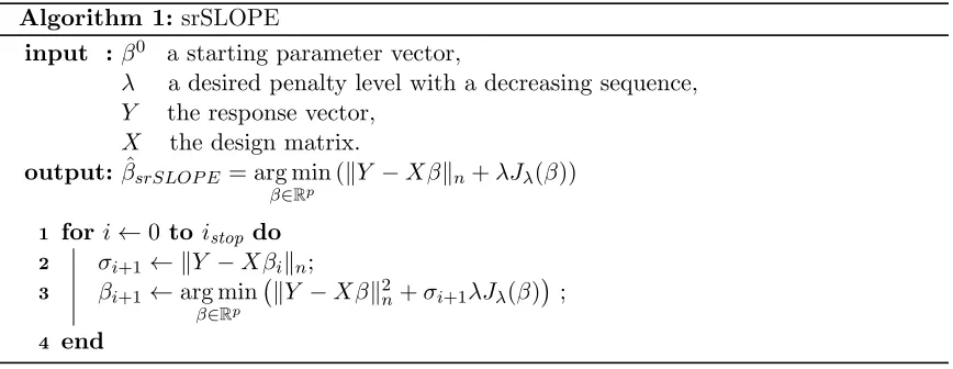
The goal of this simulation is to see how the estimation and prediction errors for the square root LASSO and the square root SLOPE behave under some Gaussian designs. We propose Algorithm 1 to solve the square root SLOPE:
Algorithm 1:srSLOPE
input :β0 a starting parameter vector,
λ a desired penalty level with a decreasing sequence,
Y the response vector,
X the design matrix. output:βˆsrSLOP E = arg min
β∈Rp
(kY −Xβkn+λJλ(β))
1 fori←0 to istop do 2 σi+1← kY −Xβikn; 3 βi+1 ←arg min
β∈Rp
kY −Xβk2
n+σi+1λJλ(β)
;
4 end
Note that in Algorithm 1 Line 3 we need to solve the usual SLOPE. To solve the SLOPE we have used the algorithm provided in Bogdan et al. (2015). For the square root LASSO we have used the R-Package flare by Li et al. (2014).
We consider a high-dimensional linear regression model:
Y =Xβ0+,
with n= 100 response variables and p = 500 unknown parameters. The design matrix X
is chosen with the rows being fixed i.i.d. realizations from N(0,Σ). Here the covariance matrix Σ has a Toeplitz structure
Σi,j = 0.9|i−j|.
We choose i.i.d. Gaussian errors with a variance ofσ2 = 1. For the underlying unknown parameter vector β0 we choose different settings. For each such setting we calculate the square root LASSO and the square root SLOPE with the theoretical λgiven in this paper and the λ from a 8-fold Cross-validation on the mean squared prediction error. We use
Decreasing Case:
Here the active set is chosen asS0={1,2,3, ...,7}, andβS00 = (4, 3.6, 3.3, 3, 2.6, 2.3, 2)
T
is a decreasing sequence.
Table 1: Decreasing β
theoreticalλ Cross-validatedλ
kβ0−βˆk
`1 Jλ(β
0−βˆ) kX(β0−βˆ)k `2 kβ
0−βˆk
`1 Jλ(β
0−βˆ) kX(β0−βˆ)k `2
srSLOPE 2.06 0.21 4.12 2.37 0.26 3.88
srLASSO 1.85 0.19 5.51 1.78 0.19 5.05
Decreasing Random Case:
The active set was randomly chosen to beS0 ={154,129,276,29,233,240,402} and again
βS0
0 = (4, 3.6, 3.3, 3, 2.6, 2.3, 2)
T.
Table 2: Decreasing Random β
theoreticalλ Cross-validatedλ
kβ0−βˆk`1 Jλ(β
0−βˆ) kX(β0−βˆ)k `2 kβ
0−βˆk
`1 Jλ(β
0−βˆ) kX(β0−βˆ)k `2
srSLOPE 4.50 0.49 7.74 7.87 1.09 7.68
srLASSO 8.48 0.89 29.47 7.81 0.85 9.19
Grouped Case:
Now in order to see if the square root SLOPE can catch grouped variables better than the square root LASSO we look at an active set S0 = {1,2,3, ...,7} together with βS00 =
(4,4,4,3,3,2,2)T.
Table 3: Grouped β
theoreticalλ Cross-validatedλ
kβ0−βˆk`1 Jλ(β
0−βˆ) kX(β0−βˆ)k `2 kβ
0−βˆk
`1 Jλ(β
0−βˆ) kX(β0−βˆ)k `2
srSLOPE 2.81 0.29 6.43 1.71 0.18 3.65
srLASSO 3.02 0.31 8.37 1.83 0.19 4.25
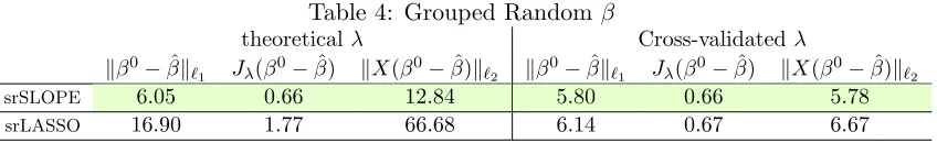
Grouped Random Case:
Again we take the same randomly chosen set S0 = {154,129,276,29,233,240,402} with
β0
S0 = (4,4,4,3,3,2,2)
T.
Table 4: Grouped Randomβ
theoreticalλ Cross-validatedλ
kβ0−βˆk
`1 Jλ(β
0−βˆ) kX(β0−βˆ)k `2 kβ
0−βˆk
`1 Jλ(β
0−βˆ) kX(β0−βˆ)k `2
srSLOPE 6.05 0.66 12.84 5.80 0.66 5.78
srLASSO 16.90 1.77 66.68 6.14 0.67 6.67
the square root LASSO in the cases where β0 is somewhat grouped (grouped in the sense that amplitudes of same magnitude appear). This is due to the structure of the sorted
`1−norm, which has some of the sparsity properties of`1 as well as some of the grouping properties of`∞, see Zeng and Figueiredo (2014). Therefore the square root SLOPE reflects
the underlying sparsity structure in the grouped cases. What is also remarkable is that the square root SLOPE always has a better mean squared prediction error than the square root LASSO. This is even in cases, where square root LASSO has better estimation errors. The estimation errors seem to be better for the square root LASSO in the decreasing cases.
6. Discussion
Sparsity inducing norms different from `1 may be used to facilitate the interpretation of the results. Depending on the sparsity structure we have provided sharp oracle inequali-ties for square root regularization. Due to the square root regularizing we do not need to estimate the variance, the estimators are all pivotal. Moreover, because the penalty is a norm the optimization problems are all convex, which is a practical advantage when imple-menting the estimation procedures. For these sharp oracle inequalities we only needed the weak decomposability and not the decomposability property of the `1−norm. The weak decomposability generalizes the desired property of promoting an estimated parameter vec-tor with a sparse structure. The structure of the Ω− and ΩSc−norms influence the oracle bound. Therefore it is useful to use norms that reflect the true underlying sparsity structure.
Acknowledgments
References
F.R. Bach, R. Jenatton, J. Mairal, and G. Obozinski. Optimization with sparsity-inducing penalties. Foundations and TrendsR in Machine Learning, 4(1):1–106, 2012.
H. H. Bauschke and P. L. Combettes. Convex analysis and monotone operator theory in Hilbert spaces. CMS Books in Mathematics/Ouvrages de Math´ematiques de la SMC. Springer, New York, 2011. With a foreword by H´edy Attouch.
A. Belloni, V. Chernozhukov, and L. Wang. Square-root lasso: pivotal recovery of sparse signals via conic programming. Biometrika, 98(4):791–806, 2011.
A. Belloni, V. Chernozhukov, and L. Wang. Pivotal estimation via square-root Lasso in nonparametric regression. The Annals of Statistics, 42(2):757–788, 2014.
P. J. Bickel, Y. Ritov, and A. B. Tsybakov. Simultaneous analysis of lasso and Dantzig selector. The Annals of Statistics, 37(4):1705–1732, 2009.
M. Bogdan, E. van den Berg, C. Sabatti, W. Su, and E.J. Cand`es. SLOPE—adaptive variable selection via convex optimization. The Annals of Applied Statistics, 9(3):1103– 1140, 2015. URL http://statweb.stanford.edu/~candes/SortedL1/.
S. Boucheron, M. Ledoux, G. Lugosi, and P. Massart. Concentration inequalities : a nonasymptotic theory of independence. Oxford university press, 2013. ISBN 978-0-19-953525-5.
F. Bunea, A. B. Tsybakov, and M. H. Wegkamp. Aggregation and sparsity vial1 penalized least squares. In Learning theory, volume 4005 of Lecture Notes in Comput. Sci., pages 379–391. Springer, Berlin, 2006.
F. Bunea, A. B. Tsybakov, and M. H. Wegkamp. Aggregation for Gaussian regression. The Annals of Statistics, 35(4):1674–1697, 2007.
F. Bunea, J. Lederer, and Y. She. The group square-root lasso: Theoretical properties and fast algorithms. IEEE Transactions on Information Theory, 60(2):1313–1325, 2014.
P. B¨uhlmann and S. van de Geer. Statistics for High-Dimensional Data: Methods, Theory and Applications. Springer Publishing Company, Incorporated, 1st edition, 2011. ISBN 3642201911, 9783642201912.
O. Klopp. Noisy low-rank matrix completion with general sampling distribution. Bernoulli, 20(1):282–303, 2014.
V. Koltchinskii. Oracle inequalities in empirical risk minimization and sparse recovery problems, volume 2033 of Lecture Notes in Mathematics. Springer, Heidelberg, 2011. Lectures from the 38th Probability Summer School held in Saint-Flour, 2008, ´Ecole d’ ´Et´e de Probabilit´es de Saint-Flour. [Saint-Flour Probability Summer School].
B. Laurent and P. Massart. Adaptive estimation of a quadratic functional by model selec-tion. The Annals of Statistics, 28(5):pp. 1302–1338, 2000.
X. Li, T. Zhao, L. Wang, X. Yuan, and H. Liu. flare: Family of Lasso Regression, 2014. URLhttps://CRAN.R-project.org/package=flare. R package version 1.5.0.
A. Maurer and M. Pontil. Structured sparsity and generalization. Journal of Machine Learning Research, 13(1):671–690, 2012.
C.A. Micchelli, J. Morales, and M. Pontil. A family of penalty functions for structured sparsity. In J.D. Lafferty, C.K.I. Williams, J. Shawe-Taylor, R.S. Zemel, and A. Culotta, editors,Advances in Neural Information Processing Systems 23, pages 1612–1623. Curran Associates, Inc., 2010.
C.A. Micchelli, J. Morales, and M. Pontil. Regularizers for structured sparsity. Advances in Computational Mathematics, 38(3):455–489, 2013.
A. B. Owen. A robust hybrid of lasso and ridge regression. In Prediction and discovery, volume 443 ofContemp. Math., pages 59–71. Amer. Math. Soc., Providence, RI, 2007.
N. Simon, J. Friedman, T. Hastie, and R. Tibshirani. A sparse-group lasso. Journal of Computational and Graphical Statistics, 2013.
W. Su and E. Cand`es. SLOPE is adaptive to unknown sparsity and asymptotically minimax.
Ann. Statist., 44(3):1038–1068, 2016.
T. Sun and C. Zhang. Scaled sparse linear regression. Biometrika, 99(4):879–898, 2012.
R. Tibshirani. Regression shrinkage and selection via the lasso. Journal of the Royal Statistical Society. Series B. Methodological, 58(1):267–288, 1996.
S. van de Geer. The deterministic lasso. JSM proceedings, 2007.
S. van de Geer. Weakly decomposable regularization penalties and structured sparsity.
Scand. J. Stat., 41(1):72–86, 2014.
S. van de Geer. Estimation and Testing under Sparsity. ´Ecole d’ ´Ete de Saint-Flour XLV. Springer (to appear), 2016.
S. van de Geer and J. Lederer. The Lasso, correlated design, and improved oracle inequal-ities. 9:303–316, 2013.
X. Zeng and M. A. T. Figueiredo. Decreasing weighted sorted l1 regularization. IEEE Signal Processing Letters, 21(10):1240–1244, June 2014.