Multi-Objective for a Partial Flexible Open
Shop Scheduling Problem using Hybrid Based
Particle Swarm Algorithm and Ant Colony
Optimization
N. Jananeeswari
1, Dr.S.Jayakumar
2and Dr.M.Nagamani
31
Research Scholar of Mathematics, Aringar Anna government Arts college, Cheyyar, Tiruvannamalai, India.
2 Assistant Professor of Mathematics, Aringar Anna government Arts college, Cheyyar, Tiruvannamalai, India.
3 Associate Professor of Mathematics, Global Institute of Engineering & Technology, Vellore, Tamilnadu, India
Abstract:
Objectives: Using the multi-objective method is to solve the partial flexible open-shop scheduling problem (PFOSP), this paper optimizes the three objectives of minimizing the makespan, the maximum workload and the total workload of machine, Methods and Statistical Analysis: analyzes the relations between the three optimization objectives in detail, and decides to Findings: minimize the makespan and the maximum workload during the process route selection and to minimize the total workload of machine processing time during the process scheduling. According to the characteristics of multi-objective optimization, the author redesigns the update mode and state transition probabilistic formula for local meta-heuristic information of ant in the optimized ant colony algorithm. Application /Improvements: The simulation experiment proves the based effectiveness of the mixed optimization algorithm of ant colony algorithm and particle swarm algorithm.
Keywords: multi-objective optimization, partial flexible open-shop scheduling, ant colony algorithm,particle swarm algorithm, process scheduling.
1. Introduction
Production scheduling is undoubtedly the core of production management in an enterprise because it maximizes the utilization of resources through scientific allocation. According to historical statistics, the non-processing operations take up 95% of the time spent on the whole production process. Therefore, scientific scheduling of production can effectively promote the production efficiency of the enterprise (Rupp et al.,2010). However, since actual environmental conditions are often constrained in theoretical research, the theoretical models of production scheduling differ greatly from the reality and yield limited practical value. In actual scheduling, the scheduler has to rely on his/her own experience to make decisions, which is difficult to deal with emergencies, thus affecting the normal production. So, it is necessary to explore how to optimize production scheduling, so as to provide basis for decision-making on scientific scheduling.
Partial Flexible Open-shop scheduling problem (PFOSP) adapts well to complex production scheduling. To be more specific:
1. From the competitive environment of manufacturing enterprises, flexible production helps the enterprises make better response to the changing market. To enhance core competitiveness, an enterprise must be capable of dealing with emergencies like equipment failure, urgent orders and temporary cancellation, etc.
2. From the angle of production technology, recent years has seen the rapid development of automation technology (Sa´nchez-Caballero et al., 2009). In particular, the emergence of partial flexible manufacturing system (PFMS) has pushed through the limitation of traditional way of process-based processing, allowing the same product to be processed simultaneously on several processing lines. Besides, during production and processing, different departments of the enterprise have different demands of scheduling. For example,
The production department wishes to reduce cost, improve efficiency and complete orders on time, the business department gives concern to the delivery time, while the senior management wants to maximize the utilization of resources and minimize waste (Liu et al., 2010). As a result, it is necessary to balance the rights and interests between different departments through production scheduling, thereby achieving the optimal manufacturing effect.
to complex production environment (Weglarz and Jozefowska, 1998). Therefore, it is of great practical and theoretical significance to study multi-objective PFOSP.
2. Partial Flexible Open Scheduling Problem
1. The research on scheduling optimization multi criteria leans heavily towards performance indices, and away from cost indices. Currently, there is little research on storage and production costs, which are critically important for measuring the scheduling level of the enterprise (Marler and Arora, 2004).
2. The research on PFOSP models lacks diversity. Most of the research is related to math and grammar-based models, while virtually no research is about PFOSP framework models.
3. There is little systematic research on PFOSP optimization theory, especially on the convergence of the algorithm, and the diversity of the solution, both of which are the key and difficult points in the field of the optimization method (Huang et al., 2006).
4. Multi-objective research on partial flexible scheduling is mostly based on an important condition, that is, all the products have the same processing objective. However, the research on the conflict between products with different processing objectives is far from mature. Even less literature talks about multi-objective optimization method where there is significant difference between large batches of products.
5. Many researchers have studied dynamic scheduling, but most of them are limited to single-objective dynamic scheduling. Very few problems into real-time, objective, dynamic scheduling optimization, or multi-objective scheduling.
3. Hybrid Optimization
Algorithm
of
Ant Colony
Algorithm
and
Particle Swarm Algorithm for Multi-Objective PFOSP
3.1 Mathematical formulation of multi-objective PFOSP
Mathematically speaking, the multi-objective PFOSP is expressed as follows. There are n products to be processed on m machines. For every Ji product, there are ni processes which are arranged in fixed order. The processes can take place in one of the m machines. Mij refers to the set of machines for the process i of product Ji. The set relation is Mij={1, 2…, M}. Oijk refers to the processing of process i corresponding to product j on machine Mk. The processing time of process i corresponding the product j is represented by pijk. In this case, j falls between 1 and n, i between 1 and nj, and k between 1 and m. The scheduling problem mainly involves two sub-problems, one is the allocation of machines, the other is the optimization of processes.
To solve the former sub-problem, the processes should be assigned to each processing machine; to solve the latter sub-problem, overall optimization should be achieved based on the processing sequence. During processing, the following restrictions and assumptions should be satisfied:
1. All of the processing machines are utilization when time t=0; 2. At this time, all semi-finished products can be processed;
3. The processing times of all processes involved on the corresponding processing machines are known(Ahmadi et al., 2013; Seyed and Sadeghiazad, 2016; Kesavan et al., 2016; Rafiee and Sadeghiazad, 2016);
4. The processing sequences of all products are known;
5. At the same time, each process must corresponds to only one machine and the processing must not be interrupted; 6. All semi-finished products are on the same level of priority, and if a product is different, the corresponding process sequence would become invalid.
To sum up, the scheduling problem can be expressed as:
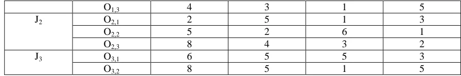
1. Complete PFOSP: when the conditions of Mij M and Oij are met, the process i of product Ji can take place on any machine in set M. Table 1 displays the complete multi-objective complete PFOSP of three products and four machines. The data in the table illustrate pijk, the processing time of the process on the corresponding machine, and the data on each row stands for the set of Mij.
Table 1 Multi-objective PFOSP (Example 1)
Jobs(3×4) Machines M1 M2 M3 M4
J1 O1,1 1 3 5 4
O1,3 4 3 1 5
J2 O2,1 2 5 1 3
O2,2 5 2 6 1
O2,3 8 4 3 2
J3 O3,1 6 5 5 3
O3,2 8 5 1 5
2. Partial FOSP: when the conditions of Mij and Oijare met, the process i of product Ji can only take place on some of the machines. Table 2 displays the details on partial multi-objective complete PFOSP of three products and four machines. The data in the table maps pijk, the processing time of the process. Means process Oij cannot take place on equipment Mk. The data in each row maps the set of Mij.
Table 2 Multi-objective PFOSP (Example 2)
Jobs(3×4) Machines M1 M2 M3 M4
J1 O1,1 - 3 2 4
O1,2 4 - - 2
O1,3 5 2 1 3
J2 O2,1 - 4 3 -
O2,2 5 - - 2
O2,3 2 2 - 5
J3 O3,1 3 3 5 3
O3,2 6 - 2 1
3.2 Mathematical model and optimization objectives
Multi-objective PFOSP needs to be optimized according to the specific requirements. The objectives are as follows:
(1) The longest processing time:
……… (1) (2) The maximum lead/lag of product delivery, a measure of the satisfaction of delivery time:
………. (2) (3) The minimum lead/lag of product delivery, an indication of the satisfaction of delivery time:
= = } ………... (3)
(4)The storage cost of semi-finished products, where F3 and F4 correspond to the cost of production:
= .(4)
(5) The sum of the load of processing machines:
……… (5)
(6) The maximum load of key machines:
……….. (6)
As mentioned above, PFOSP optimization aims at improving three objectives simultaneously. Similar to other multi-objective optimizations, there is some contradiction between the functions of multiple optimization objectives. Thus, it is impossible to get the most optimal solutions for all objectives. At this point, it is necessary to build a set of Pareto optimal solutions, i.e. compromised solutions for multi-objective optimization functions. The following formulas illustrate the constraints for the optimization objectives:
] ………... (8)
……… (9)
………..……… (10)
= 0 ………. (11)
……….. (12)
………... (13)
………... (14)
In the above formulas, Cj stands for the completion time of product Ji; dj stands for the delivery time of product
Ji; T
*
stands for the maximum completion time of the optimal scheduling; Cv stands for the actual cost of the machine; Cs stands for the static cost of the machine if it is in static state; Cp stands for the total processing cost of the manufacturing workshop, which equals Cv+Cs; STij stands for the start time of processing corresponding to process Oijk; Pijk stands for the equipment processing time of process i of product Ji; Xijk stands for the decision variable, indicating whether to use machine k for process i of product Ji (if the variable equals 1, it means machine k is used; if the variable equals 0, it means machine k is not selected); stands for the dynamic cost of equipment k; stands for the static cost of equipment k; Cwip stands for the storage cost of the product during processing; stands for the raw material cost of product Ji; and µij stands for the ratio between processing and storage cost and the total value of products in the time interval.
3.3 Multi-objective PFOSP algorithm
In the ant colony optimization algorithm, the main parameters include: Qa (the scale of ant colony), ρ (volatilization rate of pheromone), τmax(maximum concentration of pheromone) and τmin (minimum concentration of pheromone). In the particle swarm optimization algorithm, the core parameters include: Qp (the scale of particle population), NC (the maximum iterations under the algorithm), and NQ (continuous invariant algebra to achieve the optimal solution)(Sedenka and Raida, 2010). The multi-objective PFOSP algorithm is described as follows:
Step 1: Initialize the ant colony algorithm, generate an ant by a random function and denote it with letter a. Use counter r to count the number of ants by the algorithm of r=r+1. The set of products passed by ant a is denoted by tabua ( tabua =φ).
Step 2: Select the machine corresponding to product process. Specifically speaking, when a enters product i by random, count the number of processes passed by a and start the initialization process (j=0). The transition probability of the machine in the first process is Pmj,mj+1a(j). Thus, the processing machine of the first process can be determined by roulette wheel selection method (Laukkanen et al., 2012). At this moment, a starts to enter the first process, the counter reads j=j+1. The machines of the other processes can be deduced by analogy as a passes through all processes of the product. In other words, repeat this step over and over till tabua={1,2,...,N} is all passed through. Now, since the process route of the product is clear, proceed with the next step.
Step 3: Particle swarm optimization algorithm. Initialize the particle swarm and use Qp to denote the scale of the particle swarm optimization. The initialization process mainly aims at initializing the particle components of the process information chosen by ant a. The components include process, machine, product number and processing time, etc. The random initialization priority and particle velocity vector fall in the interval of 0 to 1. Next, decode the particle vector and calculate the particle fitness by the formula ; if the f
value of the particle is within the historical optimal value fgbest, replace pbest with this particle, which stands for the historical optimal individual. If the f value of the particle is better than the global optimal individual fitness fgbest, update the gbest of the individual.
under the ant colony optimization algorithm should be updated. If r<Qa, go back to Step 1. If r=Qa, go back to the beginning of this step, and set Tqbest as the minimum processing time by local iteration algorithm under ant colony optimization. Otherwise, skip to the next step.
Step 5: Calculate the velocity and position vectors of the particles. When wϵ(0,1), C1=C2=2,go back to the third step again.
Step 6: Update the pheromone concentration under ant colony algorithm. Assuming that Tbest>Tqbest, the two parameters can be set equal and the original Sbest solution should be replaced with Sq. The total processing time under Sbest is denoted by Tbest. Next, update the pheromone on the related product structure (Kuroda et al., 2015). Finally, start the iteration, let q = q + 1, if q is greater than NC, then the iterative algorithm is over, otherwise go back to the first step, and r becomes 0. q records the number of iterations in the ant colony algorithm, which falls between 1 and NC.
4. Simulation Experimental Analysis
4.1 Result Analysis 1
In the following, verify the effectiveness of mixed optimization algorithm of ant colony algorithm and particle swarm algorithm. First, introduce the PFOSP test examples (example 1: 3 machines, 3 products; example 2: 3 machines, 4 products.)
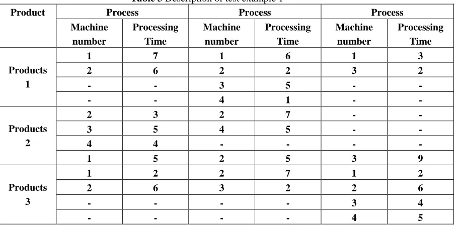
Table 3 Description of test example 1
Product Process Process Process
Machine number
Processing Time
Machine number
Processing Time
Machine number
Processing Time
Products 1
1 7 1 6 1 3
2 6 2 2 3 2
- - 3 5 - -
- - 4 1 - -
Products 2
2 3 2 7 - -
3 5 4 5 - -
4 4 - - - -
1 5 2 5 3 9
Products
3
1 2 2 7 1 2
2 6 3 2 2 6
- - - - 3 4
- - - - 4 5
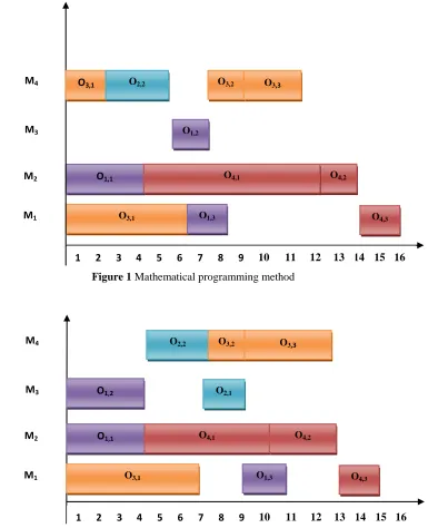
The table 3 illustrates the processing times corresponding to the processes. The results are obtained by the mathematical programming method (seen in Figure 1). Figure 2 displays the results of the mixed optimization algorithm. The total processing times are consistent with the results obtained by the mathematical programming method, both of which are 16d. However, the corresponding process routers are different. The former, the mixed optimization algorithm, has a higher machine utilization rate (Nicolaou et al., 2012). See Table 4 to compare the results between the mixed optimization algorithm and the mathematical programming method. This table shows the former has a shorter total processing time, 2d shorter, and a significantly higher machine utilization rate.
Table 4 Comparison between the results of different algorithms
Algorithm Processing
time
Total Processing time
Utilization rate of Machines
M1 M2 M3 M4 M5
Mathematical
programming method
15 45 75% 100% 75% 100% 85%
Figure 1 Mathematical programming method
Figure 2 Ant colony Algorithm
4.2 Results Analysis 2
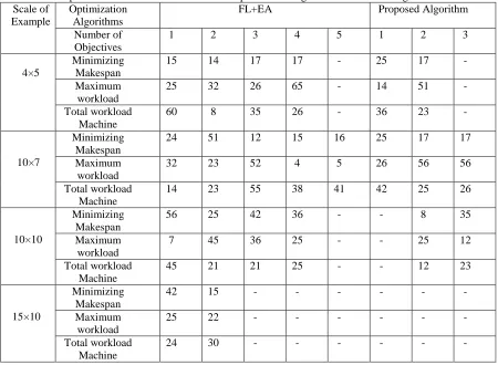
This section compares the proposed mixed optimization algorithm and the AL+CEA algorithm. The latter is put forward by Kacem et al., 3 PFOSP test problems of different scales are used. The examples corresponding to these problems respectively contain 8, 10 and 15 products, and 8, 10 and 10 machines. Conduct 30 iterative computations for these examples and compare the results of proposed method with those of other methods. In example 1, the results of each iteration are better than the later one. In example 2, the proposed algorithm has a better solution than other algorithms, indicating that the solution is an optimal solution (Nicolaou and Kannas, 2011). To solve the multi-objective PFOSP, Kacem et al. also introduce the evolutionary and fuzzy algorithm, which is the combination of FL + EA and Pareto. Next, use examples that respectively contain 4, 7, 10 and 15 products and 5, 7, 10 and 10 machines, and compare the results of different algorithms. Table 5 compares the results of the mixed optimization algorithm and the FL+EA algorithm. Although none of the maximum iterations, reasonable run-time solution quality and the average computation time is displayed in this table, it still demonstrates how the mixed optimization algorithm improves the solution quality.
O4,2
14 10
1 2 3 7
8 1
9 4
5 6 11 12 13
M1 O3,1 O1,3
M2 O1,1
M3
15 16 O4,3
O4,1
O1,2 O3,1 O2,2
M4 O3,2 O3,3
10
1 2 3 7
8 1
9 4
5 6 11 12 13
M1 O3,1 O1,3
M2 O1,1 O4,1 O4,2
O2,1 O1,2
O2,2
M3
M4 O3,2 O3,3
Table 5 Comparison between the results of mixed optimization algorithm and FL+EAalgorithm Scale of
Example
Optimization Algorithms
FL+EA Proposed Algorithm
Number of Objectives
1 2 3 4 5 1 2 3
4×5
Minimizing Makespan
15 14 17 17 - 25 17 -
Maximum workload
25 32 26 65 - 14 51 -
Total workload Machine
60 8 35 26 - 36 23 -
10×7
Minimizing Makespan
24 51 12 15 16 25 17 17
Maximum workload
32 23 52 4 5 26 56 56
Total workload Machine
14 23 55 38 41 42 25 26
10×10
Minimizing Makespan
56 25 42 36 - - 8 35
Maximum workload
7 45 36 25 - - 25 12
Total workload Machine
45 21 21 25 - - 12 23
15×10
Minimizing Makespan
42 15 - - - -
Maximum workload
25 22 - - - -
Total workload Machine
24 30 - - - -
5. Conclusion
Using a mixed optimization algorithm of ant colony algorithm and particle swarm algorithm is applied to solve the multi-objective PFOSP; this paper optimizes the three interrelated objectives of minimizing makespan, maximum workload; Total workload of machines. The total machine load and key machine load are minimized through the finding the optimal process route. In the meantime, this paper redesigns the update formula of ant colony transition probability in light of the multi-objective optimization attributes. The total processing time is optimized during process scheduling. Particle swarm optimization algorithm is applied at this stage, and the related problems are adjusted by the decoding and particle coding. Finally, the author obtains the Gantt chart of the proposed optimization algorithm, and compares the results of the algorithm with those in other materials. The experiment proves that the proposed mixed optimization algorithm has a significant effect on solving multi-objective PFOSP, and can also effectively enhance machine utilization rate.
6. REFERENCES
[1] Ahmadi M.H., Hosseinzade H., Sayyaadi H., Mohammadi A.H., Kimiaghalam F. (2013). Application of the multi-objective optimization method for designing a powered stirling heat engine: design with maximized power, thermal efficiency and minimized pressure loss. Renewable Energy, 60(4), 313-322.
[2] Huang H.Z., Gu Y.K., Du X. (2006). An interactive fuzzy multi-objective optimization method for engineering design. Engineering Applications of Artificial Intelligence, 19(5), 451-460.
[3] Kuroda K., Magori H., Ichimura T., Yokoyama R. (2015). A hybrid multi-objective optimization method considering optimization problems in power distribution systems. Journal of Modern Power Systems and Clean Energy, 3(1), 41-50.
[4] Kesavan E., Gowthaman N., Tharani S., Manoharan S., Arunkumar E. (2016). Design and Implementation of Internal Model Control and Particle Swarm Optimization Based PID for Heat Exchanger System, International Journal of Heat and Technology, 34(3): 386-390.
[5] Laukkanen T., Tveit T.M., Ojalehto V., Miettinen K., Fogelholm C.J. (2012). Bilevel heat exchanger network synthesis with an interactive multi-objective optimization method. Applied Thermal Engineering, 48(26), 301–316.
[6] Liu C., Peng W., Shi H. (2010). The study of scheduling rules for spraying and drying processes scheduling in painting worksh op, 2, 605-608.
[7] Marler R.T., Arora J.S. (2004). Survey of multi-objective optimization methods for engineering. Structural & Multidisciplinary Optimization, 26(6), 369-395.
[9] Nicolaou C. A., Brown N. (2013). Multi-objective optimization methods in drug design. Drug Discovery Today Technologies, 10(3), 427-35.
[10] Nicolaou C.A., Kannas C.C. (2011). Molecular library design using multi-objective optimization methods. Methods in Molecular Biology, 685(685), 53-69.
[11] Nicolaou C.A., Kannas C., Loizidou E. (2012). Multi-objective optimization methods in de novo drug design. Mini Reviews in Medicinal Chemistry, 12(10), 979-987(9).
[12] Rafiee S.E., Sadeghiazad M.M. (2016). Three-Dimensional CFD Simulation of Fluid Flow inside a Vortex Tube on Basis of an Experimental Model- The Optimization of Vortex Chamber Radius, International Journal of Heat and Technology, 34(23): 236-244. [13] Rupp B., Pauli D., Feller S., Skyttä M. (2010). Workshop scheduling in the mro context, 1281(1), 2000-2003.
[14] Sa´nchez-Caballero S., Boronat-Vitoria T., Marti´nez-Sanz A.V., Colomer-Romero V., Sa´nchez-Caballero S., Boronat-Vitoria T., (2009). Mechanical workshop scheduling using genetic algorithms, 1181(1), 775-785.
[15] Sedenka V., Raida Z. (2010). Critical comparison of multi-objective optimization methods: genetic algorithms versus swarm intelligence. Radio engineering, 19(3), 369-377.
[16] Seyed E.R., Sadeghiazad M.M. (2016). Heat and Mass Transfer Between Cold and Hot Vortex Cores inside Ranque-Hilsch Vortex Tube-Optimization of Hot Tube Length, International Journal of Heat and Technology, 34(1): 31-38.
[17] Weglarz J., Jozefowska J. (1998). Fifth international workshop on project management and scheduling. European Journal of Operational Research, 107(2), 247-249.
[18] Xun J., Ning B., Li K.P. (2008). Multi-objective optimization method for the auto system using cellular automata. Computers in Railways XI, 173-182.
[19] Zhang R., Xie W.M., Yu H.Q., Li W.W. (2014). Optimizing municipal wastewater treatment plants using an improved multi-objective optimization method. Bioresource Technology, 157(157), 161-165.
[20] ZhangY., Squillante M. S., Sivasubramaniam A., Sahoo R. K. (2004). Performance Implications of Failures in Large-Scale Cluster Scheduling. Job Scheduling Strategies for Parallel Processing, International Workshop, 3277, 233-252.
[21] Zheng F., Zecchin A. (2014). An efficient decomposition and dual-stage multi-objective optimization method for water distribution