I. Introduction
I
N recent years, cloud environments are increasingly used in the scientific field [1]. These environments are currently changing dramatically because of the integration of new technologies such as GPUs, sensors, etc.; thus providing scientists with high computing power, storage, and bandwidth. However, the drawback of this power lies in the heterogeneity of resources that makes its management more complex. Other complexities arise because of the urgent need for scale-up, reduced application response time, fault tolerance and infinite storage space, which pushes scientists to use multiple applications simultaneously, resources at the same time in a Workflow application.Scientific workflows are used to model computationally intensive and large-scale data analysis applications [2]. In recent years, cloud computing has been evolving rapidly as a target platform for such applications [3]. As a result, several workflow-specific resource management systems have been developed by cloud providers, such as the Amazon Simple Workflow Service (SWF) [4], to enable users to dynamically provision resources.
The workflow-scheduling problem has been studied extensively over past years focusing on multiprocessor system and distributed
environments like grids and clusters [5]. Workflow and directed acyclic graph (DAG) are usually interchangeable in the literature. It is a well-known research area where the programming complexity is NP-complete. [6].
The Workflow scheduling approaches can be classified according to different aspects of optimization method such as heuristic, clustering, critical path, fuzzy, greedy, market-driven, meta-heuristic, mathematical modeling, and partitioning. Majority of the Workflow scheduling approaches focus on employing heuristic and meta-heuristic as an optimization method and focusing only on the execution time [7]. However, even in these cases, communication among tasks is assumed to take zero time units. In our approach, we use Clustering scheduling to achieve a better performance regarding effectiveness and accuracy at the cost. Clustering-based scheduling is designed to optimize transmission time between data dependent tasks [8]. DAG Clustering is a mapping of all tasks onto clusters, where each cluster is a subset of Tasks, and each cluster is executed on a separate resource. The basic idea of clustering is to reduce the communication time between tasks.
Traditional techniques have examined the data sharing of workflows tasks. These techniques that investigate the scheduling of scientific workflows tasks have inspired us when developing our approach. However, the tasks hierarchy in scientific workflows has not been explored extensively. Therefore, we consider in this paper the tasks hierarchy for workflow scheduling.
Keywords
Cloud Computing, Workflow Data Scheduling, Clustering, Data Transformation, Clustering Quality Indexes, CloudSim.Abstract
Scientific workflows benefit from the cloud computing paradigm, which offers access to virtual resources provisioned on pay-as-you-go and on-demand basis. Minimizing resources costs to meet user’s budget is very important in a cloud environment. Several optimization approaches have been proposed to improve the performance and the cost of data-intensive scientific Workflow Scheduling (DiSWS) in cloud computing. However, in the literature, the majority of the DiSWS approaches focused on the use of heuristic and meta-heuristic as an optimization method. Furthermore, the tasks hierarchy in data-intensive scientific workflows has not been extensively explored in the current literature. Specifically, in this paper, a data-intensive scientific workflow is represented as a hierarchy, which specifies hierarchical relations between workflow tasks, and an approach for data-intensive workflow scheduling applications is proposed. In this approach, first, the datasets and workflow tasks are modeled as a conditional probability matrix (CPM). Second, several data transformation and hierarchical clustering are applied to the CPM structure to determine the minimum number of virtual machines needed for the workflow execution. In this approach, the hierarchical clustering is done with respect to the budget imposed by the user. After data transformation and hierarchical clustering, the amount of data transmitted between clusters can be reduced, which can improve cost and makespan of the workflow by optimizing the use of virtual resources and network bandwidth. The performance and cost are analyzed using an extension of Cloudsim simulation tool and compared with existing multi-objective approaches. The results demonstrate that our approach reduces resources cost with respect to the user budgets.
* Corresponding author.
E-mail address: [email protected]
DOI: 10.9781/ijimai.2018.07.002
Data-Aware Scheduling Strategy for Scientific
Workflow Applications in IaaS Cloud Computing
Sid Ahmed Makhlouf*, Belabbas Yagoubi
L.I.O. Laboratory, Department of Computer Science, Faculty of Exact and Applied Sciences, University
of Oran1 Ahmed Ben Bella, P.O. Box 1524 El M’Naouer, Oran (Algeria)
The existing scheduling techniques have been categorized into three parameters including static, dynamic, and static-dynamic. Dynamic scheduling is efficient for a cloud computing environment due to its ability to handle the arriving tasks [7]. Moreover, hierarchical scheduling cooperates static and dynamic scheduling to generate powerful solutions [8].
To address the challenge, we propose a novel approach for workflow scheduling considering the hierarchy of scientific workflows tasks. Significant contributions presented in this paper are summarized as follows:
• Conditional probability for scientific workflows tasks is computed leveraging their representation as a matrix. The conditional probability reflects the possibility that scientific workflow tasks can share or use the same data.
• Determining the exact number of workflow clusters using 13 clustering indexes. In this work, we focus on the following research question: What is the number of virtual machines required for the efficient and transparent execution of a workflow in a cloud environment?
• Do a hierarchical clustering to determine the tasks hierarchy in scientific workflows and to regroup the workflow tasks into clusters. To minimize data transfer between clusters we have measured the distance between each pair of tasks and regroup the closer tasks into the same cluster.
• Extensive experiments are conducted for evaluating the effectiveness and accuracy of our technique. The result shows that our approach reduces the resources cost and total the data transfer time.
The paper is organized as follows. Section II presents related work. Section III describes the problem statement and introduces the proposed solution. In Section IV we introduce our system model and assumptions. Section V contains a description of our proposed approach, and Section VI and VII discuss the evaluation procedure and the results by applying our approach. Finally, Section VIII outlines general conclusions and exposes our future work.
II. Related Works
In the literature, researchers classify task-scheduling strategies into two main classes: job scheduling, that focuses on scheduling a set of independent tasks to be executed sequentially or in parallel, and the workflow that map and manage the execution of interdependent tasks on shared resources. Since the advent of cloud computing, several scheduling techniques for workflow applications have been proposed. These techniques take into account many aspects of the cloud environment. For example, some techniques try to optimize costs, while others try to optimize fault tolerance.
The cost has become an important objective in workflow cloud scheduling research. The total cost incurred by running workflow can include many components such as the cost of computing resources, the cost of storage resources, and the cost of data transfer resources. A budget is often defined as the number of the maximum virtual machines to process workflow. Also in grid computing, several cost-aware scheduling techniques have been introduced [9]. In [10], the authors introduce a strategy called ADAS (Adaptive Data Scheduling) for workflow applications. This work aims to reduce the monetary cost of moving data while a workflow is running. The authors propose adaptive scheduling based on dependencies between tasks. The scheduling process is in two steps; The first one is to create initial clusters for workflow tasks. They use a matrix approach to group tasks in some data centers as initial clusters using the BEA algorithm (Bond Energy Algorithm) [11]. The second step is to group the data/task pairs using the cost-effective scheduling quality. The authors demonstrate that this
strategy can improve the processing time of a workflow and the use of resources in a cloud environment. However, this strategy uses only one clustering algorithm (BEA) to create clusters; in our strategy, we use 13 clustering indexes to determine the specific clusters numbers and do a hierarchical clustering to regroups workflow tasks into clusters. In [12], the authors propose a scheduling system for a data-intensive workflow to minimize its processing time. To reduce data transfer time, the proposed system uses task clustering when submitting a workflow application. To do this, it calculates the dependencies of the tasks in the workflow according to the conditional probability of the common number of files for each pair of tasks. This clustering method is validated with the simulator WorkflowSim. We note that the authors count conditional probability of the number of common files for each pair of tasks regardless of file size. So, in this strategy, it is possible to group tasks around small files only, which involves clustering tasks with a low communication rate. In our strategy, we use the conditional probability to determine and count the possible bytes number of common files for each pair of tasks. The priority is to group only those tasks that communicate through large files. Our idea is to avoid unnecessary moving large files, which will consequently speed up the execution time of the workflow.
In addition to the makespan and cost criteria, the reliability of the workflow execution is also taken into account. This criterion ensures that the resources selected in a schedule can probably complete the scheduled tasks. The failure of the task execution is usually handled by checkpointing and replication mechanisms. On the other hand, the existence of multiple replicas introduces a challenge for maintaining the replicas consistency in the cloud environment. To solve the problem of replica coherence in the cloud, in [13], the authors propose a workflow partitioning approach that takes into account data placement by grouping tasks into a cluster based on data replication in cloud environments. The proposed approach improves the placement of data and minimizes response time. According to the authors, this is due to scheduling of tasks in data centers that contain the majority of the replicated data. Replication-based scheduling approach achieves shorter makespans. However, it makes the scheduling problem more difficult. The scheduling algorithm not only needs to observe the precedence constraints between tasks but also needs to recognize which tasks and data to duplicate. In our strategy, we used the conditional probability to determine the possible common set of data between each pair of tasks. However, both mechanisms of checkpointing and replicating the task may respectively cause the waste of time and compute resources [14, 15]. Replication and checkpointing require storage space for each task and for each file in the workflow. And probably the transfer of replicas and checkpoint across the network, which increases the makespan of the workflow. In addition, these replication and checkpointing mechanisms require a reliable central or distributed storage management system. We note that none of the works cited in this paragraph measure, in terms of data storage and transfer, the impact by using the replication and the checkpointing mechanisms.
Several studies have used cluster analysis to schedule workflow tasks into clusters. Authors in [20] propose an approach for dynamic resources provisioning and present a cost- and deadline-constrained workflow scheduling algorithm in a cloud environment. The work is divided into two phases: (i) in the first phase, they use the k-means clustering technique for determining the speed of VMs that would be selected in scheduling; (ii) in the second phase, they propose an approach for dynamic provisioning of VMs using a variant of “Subset Sum” problem. The results of the simulation show that the proposed approach achieves better performance with respect to the cost of execution.
K-means is one of the most known cluster analysis algorithms. However, the most important limitations of k-means are: (i) at the beginning of algorithm, the user must specify the number of clusters -k- and choosing the number -k- of clusters can be difficult; (ii) k-means is mainly limited to Euclidean distances. In our strategy, we implement an agglomerative hierarchical clustering to find the best step at each cluster fusion to determine the best cluster number k. Hierarchical clustering does not require a specific distance measure; any measure can be used.
In most studies, data transfer between workflow tasks is not considered, data uploading and downloading are assumed as part of task execution. However, this is not always the case, especially in the big data area. For a data-intensive workflow application, data movement can dominate both the execution time and cost. In [21], cloud storage resources are virtualized like Amazon S3 resources. The S3 Cloud storage is used for data availability and data broadcasting. However, in the design of the data placement strategies for resource provisioning it is important to consider the intermediate data transfer performance explicitly. Workflow tasks communicate through the transfer of intermediate files. So, the choice of locality storage system has a significant impact on workflow performance and cost. In our strategy, we take into account the intermediate data transfer cost between tasks when the VMs (Clusters) are deployed.
Based on this literature review, we find several issues that have not been sufficiently studied. These are the gaps in the reviewed work that will be directions for our works.
In this work, we try to understand the challenges of managing virtual resources when running Scientific Workflow in the Cloud. We will try to minimize the number of resources allocated to a Workflow under budget constraints. The goal was to improve the efficiency of resource provisioning in the cloud to execute the large-scale workflow better. To do this, we have developed tasks and data clustering systems. The clustering is done in relation to the underlying network load and inter-task communication rates. We have experimented our resource allocation strategy using an extension of the CloudSim [22] simulator.
III. Problem Statement
In the distributed execution paradigm, a workflow is divided into small tasks, which are assigned to different data centers for execution. When a task requires processing of data from different data centers, data movement becomes a challenge. Some data are too large to be moved. In a cloud, data centers are geographically distant, and data movement would add monetary cost to the Workflow execution. Our work aims to reduce the monetary cost of data movements during workflow execution, to improve the use of the network in Cloud environment. The data location problem is one of the important challenges for planning a data-intensive application in Cloud Computing.
In data-intensive scientific workflows, tasks require more than one set of data to be executed. However, when these tasks are executed
in different datacenters, data transfer would become inevitable. To resolve these issues, this work proposes a task dependency-based clustering method to optimize scheduling and execution of workflows. This work proposes a data-intensive workflow scheduling system to minimize data movement between data centers. In the next section the components of the proposed system are described.
IV. System Model and Assumptions
In this section, we present the main assumptions of our approach and environment model.
A. Application Model
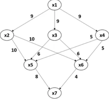
Scientific workflows are modeled as Directed Acyclic Graph (DAG). A DAG, G(V, E), consists of a set of vertices V, and edges, E. The edges represent constraints. Each edge represents a precedence constraint that indicates that the task must complete its execution before the next task begins. Each edge also represents the amount of data between tasks involved; for example, Fig. 1 shows the amount of data (in bytes) that the task should send to the next one.
A task is said to be ready if all of its parents have completed their execution and cannot begin execution until all dependencies have been satisfied. If two tasks are scheduled on the same data center, the cost of communication between them is supposed to be zero.
Applications target are Workflows. Tasks Workflow runtime is estimated, and it indicates how long it takes to execute them on a given VM type. As for execution times, we assume that the size of the files can be estimated on the basis of historical data. The files are assumed to be write-once, read-many.
A task has zero or more input files that must be fully transferred to a virtual machine before execution can begin; And has zero or more output files which can be used as inputs for another task or as the final result of a workflow. We suppose that file names are unique in a workflow.
B. Execution Model
A cloud consists of an unlimited number of virtual machines (VMs) that can be provisioned and de-provisioned on demand. A virtual machine can execute only one task at a time. A virtual machine is charged 1 $ for each interval of 60 minutes (one hour) of operation. Partial usage of a billing interval is rounded.
C. Data Transfer Model
We use a global storage model to transfer input and output files between tasks and to store the results of the Workflow. Each VM has a local cache of files. This method of transfer is widely used in cloud environments by using shared distributed file systems such as NFS
[23].
To transfer a file between virtual machines, a request must be sent to the Global Storage Management System (GSMS). The performance of transferring a file to its destination depends on the dynamic state of the underlying network. The state of the network depends on the number of files being transferred, the size of the files being transferred and the presence of the files in the local cache of the VMs.
A file cannot be transferred faster than a given maximum bandwidth. Each request to the storage system is managed with latency measured in milliseconds. We assume that we can calculate precisely the time required to transfer a file. A virtual machine has a local disk that serves as a file cache, and the disc price is included in the VM cost. The files are cached in the First-In-First-Out (FIFO) policy.
V. Proposed Approach
Tasks clustering is a technique that consolidates fine-grained tasks into coarse tasks. Task clustering has proven to be an effective method of reducing overhead costs and improving the performance of scientific workflow tasks. With task clustering, Workflow execution overhead can be eliminated by grouping small tasks into a single job unit. This Workflow reduction benefits the entire cloud environment by reducing traffic between sites. For the efficient execution of a Workflow on a cloud environment, we propose in this work, a policy of allocation and management of virtual resources. This policy is based on the calculation of the dependency between workflow tasks. The dependency is based on the conditional probability of workflow tasks.
A. Task Clustering Based on Conditional Probability
The proposed system uses tasks clustering in the Workflow to reduce data transfer time. As an illustration, we use the example of the Scientific Workflow in Fig. 1. In this Workflow, there are seven tasks. In scientific workflows, tasks communicate data by sending and receiving intermediate files. In our workflow model, we assume that the edges are files. So, we have a set of tasks T and set of files F.
In our model, first, we compute the task dependencies in the workflow based on the conditional probability. Let xi∊T and yi∊T
two tasks of the same Workflow G. It is assumed that xi has non-zero probability. The conditional probability of a task yi , knowing that another task xi has finished, is the number noted P (xi | yi) and defined
by:
(
|) (
= i( )
j)
,( )
> 0i j i
i
P x y
P x y P x
P x ∩
(1)
The real P (xi | yi) is read “probability of yi , knowing xi” according tothe common use of the sets of data between xi and yi .
Fig. 1. Example of workflow instance.
The conditional probability imposes the creation of the conditional probability matrix CPM [| T |][| T |] based on contingency table
CT [| T |+ 1][| T |+ 1] and the joint and marginal probability table
JMP [| T |+ 1][| T |+ 1] of each task pair in the workflow. First, we create contingency table as expressed in (2).
[ ][ ]
=(
{ }
Pi j,{ }
i{ }
j)
;1 ,CT i j DataSize O ∩ I ∩ I ≤i j T≤
(2)
Pi,j is the set of common parents between each tasks xi , yi :
{ }
{ }
{
}
,
=
i j i j
P
P
∩
P
(3)
Pi and Pj are respectively the parents set of the tasks xi , yi . The
dependency is calculated by measuring the total size of all the output files of the set Pi,j . OPi j, ⊂F is the set of the output files of Pi,j . Ii ∊F
and Ij ∊F are respectively inputs files set of task xi ∊T and yj ∊T. Each
value in the contingency table is the common size of the input files for each task pair in the workflow:
[ ]
[ ][ ]
=1
1 =
T;1
j
CT i T
+
∑
CT i j
≤ ≤
i T
(4)
[ ]
[ ][ ]
=1
1
=
T;1
i
CT T
+
j
∑
CT i j
≤ ≤
j T
(5)
[ ]
=1
1
1 =
T1
i
CT T
+ +
T
∑
CT i T
+
(6)
The joint and marginal probability table can be created from the contingency table. The joint probability of Ti and Tj is:[ ][ ]
=[ ][ ]
;1 ,1 1
CT i j
JMP i j i j T
CT T + + T ≤ ≤
(7)
The marginal probability of Ti is:
[ ]
1 = 1[ ]
=[ ]
11 1
CM i T
JMP i T JMP T i
CM T T
+
+ +
+ +
(8)
From Joint and Marginal Probability Table, the conditional probability for each task pair can be calculated as follows:
[ ][ ]
=[ ]
[ ][ ]
;1 ;11
JMP i j
CPM i j i T j T
JMP i T + ≤ ≤ ≤ ≤
(9)
To determine the number of clusters of the workflow, we apply our clustering approach on the CPM matrix. However, before applying any clustering method, we must first preprocess the CPM matrix data. Data pre-processing has to do with the steps that are required to transform the data we have in a way that allows applying further analysis algorithms (e.g., Clustering techniques).
B. Transforming Data
The original CPM data matrix needs to go through some modification to make it more useful for our analysis. Numeric variables sometimes have slightly different scales. This can create problems for some data analysis tools [24].
First, we identify Skewness distributions of CPM data matrix. Skewness is a measure of shape distribution. Negative skewness indicates that the mean of the data values is less than the median, so the data distribution is skewed to the left. Positive skewness indicates that the mean of the data values is larger than the median, so the data distribution is skewed to the right.
• If the skewness is equal to 0, then the data is symmetrical and did not need to be transformed.
symmetric, and need to be transformed.
• If the skewness is less than -1 or greater than +1, the data is highly skewed, and need to be transformed.
• If the skewness is between -1 and -1/2 or between +1 and +1/2 then the data is moderately skewed and need to be transformed. For example, skewness value of the workflow of Fig. 1 is 2.34, so we must do data transformation. Transforming data is used to coerce different variables to have similar distributions.
Because some measurements in nature are naturally distributed following a normal distribution, it is important to develop an approach to transforming one or more variables into a normal distribution. Other measures can be naturally logarithmic. In the literature, common data transformations include the transformation of the square root, the cube root, and the logarithm.
In data analysis, the transformation is the replacement of a variable with a function of that variable; for example, replacing a variable
x with the square root of x
( )
x or the logarithm of x (Logbx). A transformation changes the shape of distribution or relationship between variables.• The logarithm transformation transforms x to Log10 x, or x to
Logex, or x to Log2 x. It is a strong transformation with an effect on
the shape distribution. It is used to reduce the right skewness. It can not be applied to null or negative values. So we cannot apply the logarithm transformation for the CPM matrix data.
• The cube root transforms to
x
13. It is a weaker transformation than the logarithm but with a substantial effect on the shape of the distribution. It is also used to reduce right skewness and has the advantage of being able to be applied to null and negative values. • The square root transforms x to x12, is a weaker transformationthan the logarithm and cube root with a moderate effect on the distribution shape. It is used to reduce the right skewness, and also has the advantage of being able to be applied to null values. The Table I shows skewness value of square and cube root transformation. We can see that the cube root transformation approximates the normal distribution. So the cube root transformation is more powerful than the square root transformation, and we will adopt it in our experiments in section VI.
TABLE I. Different Skewness Values of Fig. 1
Original skewness square root cube root
2.340348 1.899396 1.822186
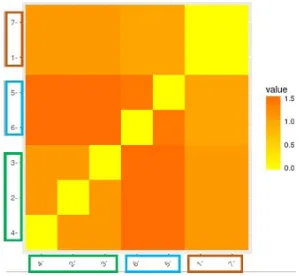
After applying our clustering approach on the CPM matrix we obtain the results of Fig. 2. In the following sections, we will discuss in detail our clustering approach used for this example.
Fig. 2. Example of workflow clustering.
After the creation of theCPM matrix, we will fragment the workflow into clusters of tasks. Each cluster will be assigned to a virtual machine, so the number of virtual machines created depends on the number of clusters. The goal of this work is to maximize the data transfer in a cluster and minimize it between clusters. The question that arises then is: What is the minimum number of clusters needed to execute the workflow to meet user budget correctly? So, in our work, the workflow execution must be efficient, meet the workflow budget and at a minimal cost. To answer this question, we have implemented some algorithms and technics for determining the optimal number of clusters in CPM dataset and offering the best workflow clustering scheme from different results.
In [25], the authors identify 30 clustering quality indexes that determine the optimal number of clusters in a dataset and offers the best clustering scheme from different results to the user. We tried to apply these 30 algorithms to our CPM matrix, and we found that only 13 algorithms are compatible with the CPM data matrix. For the rest of the 17 algorithms, the clustering result tends to infinity.
The evaluation of the algorithms on the CPM matrix must deal with problems such as the quality of the clusters, the quality of the data compared to the clustering quality indexes, the degree which a clustering quality indexes fit with the data of the CPM matrix and the optimal number of clusters [25]. As a result, we used the following clustering quality indexes:
1. Krzanowski and Lai 1988 [26]
2. Calin'ski and Harabasz 1974 [27]
3. Hartigan 1975 [28]
4. McClain and Rao 1975 [29] 5. Baker and Hubert 1975 [30]
6. Rohlf 1974 [31] and Milligan 1981 [32]
7. Dunn 1974 [33]
8. Halkidi et al. 2000 [34]
9. Halkidi and Vazirgiannis 2001 [35] 10. Hubert and Levin 1976 [36]
11. Rousseeuw 1987 [37]
12. Ball and Hall 1965 [38]
13. Milligan 1980, 1981 [39, 32]
C. Tasks Distance Measures
The data set is represented by the CPM matrix. Each element in the CPM matrix represents the distance between two tasks in the workflow. So, the clustering is done comparing the distance between each pair of tasks of the matrix CPM. To measure the distance, we used the following metrics:
Euclidean distance is the distance between two tasks x and y in a Rn space and is given by (10).
(
)
2=1
= n i i ; ,i i 1, 1,
i
d
∑
x y− x y CPM∈ T T(10)
It is the length of the diagonal segment connecting x to y.Manhattan distance is the absolute distance between tasks x and y
in Rn space and is given by (11).
=1
=
n i i; ,
i i1,
1,
i
d
∑
x y x y CPM
−
∈
T
T
Minkowski distance: is the pth root of the sum of the pth powers of
the differences between the components. For two tasks x and y in Rn
space, Minkowski distance is given by (12). 1
=1
= n p p; , 1, 1,
i i i i i
d x y− x y CPM∈ T T
∑
(12)
Minkowski distance can be considered as a generalization of both the Euclidean and the Manhattan distance [40]. p = 1 corresponds to the Manhattan distance and p = 2, to the Euclidean distance. For p reaching infinity, we obtain the Chebyshev distance.
D. Cluster Analysis Method and VMs Number Interval
As mentioned above, we used 13 partitioning algorithms to determine the exact number of clusters needed. In addition to the CPM
matrix and the distance metric, these algorithms require other input parameters, namely the cluster analysis method, the minimum and maximum cluster interval. In our works, we have used the following cluster analysis methods:
Single: The distance Dij between two clusters Ci and Cj is the
minimum distance between two tasks x and y, with x∊Ci , y∊Cj .
( )
,
=
min
,
ij
x C y Ci j
D
d x y
∈ ∈
(13)
Complete: The distance Dij between two clusters Ci and Cj is the maximum distance between two tasks x and y, with x∊Ci , y∊Cj .
( )
,=
max
,
ij x C y C i j
D
d x y
∈ ∈
(14)
We have set the cluster interval calculation between 2 and 20 clusters. This interval choice is based on the Amazon EC2 resource allocation policy [17, 18, 19]. Amazon EC2 allows the possibility of reserving only 20 virtual machines. This is why we cannot create more than 20 clusters. So, we have fixed the user budget to 20 virtual machines.
Algorithm 1 models the first step of our approach, determining the cluster number. We start by creating the CPM matrix in line 2. Then the matrix created will be one of the input parameters to the 13 clustering quality indexes cited above. In line 6 each algorithm will calculate the possible cluster number for the CPM matrix. At the end of algorithm 1, we calculate the average number of the clusters from all the proposed numbers obtained from the 13 clustering quality indexes in line 8.
E. Hierarchical Clustering Method
The average obtained will be used to do a hierarchical clustering
of the CPM matrix. Hierarchical clustering is one of the domains of automatic data analysis and data classification. Strategies for hierarchical clustering are generally divided into two types:
Agglomerative: This is a “bottom-up” approach; this method starts
from a situation where all tasks are alone in a separate cluster, then pairs of clusters are successively agglomerated until all clusters have been merged into one single cluster that contains all tasks.
Divisive: This is a “top-down” approach, in which all tasks are in a
single cluster; we divide this cluster into two sub-clusters which are, in turn, divided into two sub-clusters and so on. At each step, each cluster is divided into two new clusters.
In our work, we have used agglomerative clustering of a set of tasks
T of n individuals. Our goal is to distribute these tasks in a certain number of clusters, where each cluster represents a virtual machine.
The agglomerative hierarchical clustering assumes that there is a measure of dissimilarity between tasks; in our case, we use CPM
matrix as a measure for dissimilarity calculation. The dissimilarity between tasks x and y will be noted dissimcpm (x, y).
The agglomerative hierarchical clustering produces a hierarchy H of tasks. H it is the set of clusters at all the steps of the clustering approach and checks the following properties:
1. T∊H : at the top of the hierarchy, when grouping clusters to obtain a single cluster, all tasks are grouped;
2. ∀ x∊T, {x} ∊ H: at the bottom of the hierarchy, all tasks are alone;
3. ∀ (h,h') ∊ H 2 , h ⋂ h' = ø or h ⊂ h' or h'⊂ h
Initially, in our approach, each task forms a cluster. We try to reduce the number of clusters to the average calculated previously by the 13 clustering quality indexes; this is done iteratively. At each iteration, two clusters are merged, which involves reducing the number of total clusters.
The two clusters chosen to be merged are the most “similar”, in other words, those whose dissimilarity is minimal (or maximal). This dissimilarity value is called aggregation index. Since we first merge the closest tasks, the first iteration has a low aggregation index, but it will increase from iteration to another iteration.
For agglomerative clustering, and to decide which clusters should be merged; a measure of dissimilarity between sets of clusters is required. This is achieved by measuring a distance between pairs of clusters discussed in section V.D.
The dissimilarity of two clusters Ci = {x}, Cj = {y}; 1 ≤ i, j ≤ n , each
containing one task, is defined by the dissimilarity between its tasks
dissim(Ci, Cj) = dissim (x, y); 1 ≤ i, j ≤ n.
When clusters have several tasks, there are multiple criteria for calculating dissimilarity. We used the following criteria:
Single link: the minimum distance between tasks of Ci and Cj :
(
)
(
( )
)
,
,
=
min
,
;1 ,
i j cpm
x C y Ci j
dissim C C
dissim
x y
i j T
∈ ∈
≤
≤
(15)
We have used this method to minimize data transfer between clusters and maximize the data transfer inside a cluster.Complete link: the maximum distance between tasks of Ci and Cj :
(
)
(
( )
)
,
, = max , ;1 ,
i j x C y C cpm
i j
dissim C C dissim x y i j T
∈ ∈ ≤ ≤
we have used it to prove the performance of our workflow clustering policy.
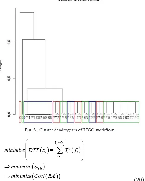
Algorithm 2 models the agglomerative hierarchical clustering of the CPM matrix. It receives as input parameters the CPM matrix and the cluster number that we want to create. The cluster number is the average of all cluster numbers obtained from the 13 clustering quality indexes. The result of hierarchical clustering is presented in a dendrogram. Fig. 3 is the result of clustering, a LIGO workflow of 50 tasks into 11 clusters using the Euclidean distance measurement and the Single Link agglomeration method.
F. Objective Function
We have introduced an objective function that allows us to know the granularity of our resource allocation system. The objective function depends on the workflow resources allocation cost. When a task xi is
assigned to a VM Vk with price pk, we refer to this as a Resources
Allocation RAi. For each RAj its cost value is computed :
( )
i= cos
(
i,
k)
=
i k, kCost RA
t x v
ω
⋅
p
(17)
Where pk is the monetary cost per hour to execute a task xi on the VM
Vk . The execution takes
ω
i k, time units. The execution time includes the transfer time of the input tasks data set to the virtual machine from task yj to the task xi.( )
I O
, ,
=0
=
i ji k i k l
l
E
T f
ω
∩
+
∑
(18)
Ei,k is the execution time of task xi on the VM vk, Ii is the input set of files of the task xi and Oj is the output set of files of the task yj. T fij
( )
lis the transfer time of file fl of the task xi to the VM vk from the task yj .
For xi ∊ Ci and yj ∊ Cj , T fij
( )
l is defined as :( )
( )
;0;
=
Size fl i j
j Bw
i l Otherwise
T f
≠
(19)
Bw is the bandwidth between cluster Ci and cluster Cj. In this work,
we aim to minimize the transfer time of the data set between the virtual machines. To do this, we try to reduce the amount of data set transferred between VM by clustering the highly connected tasks in the same cluster. By this way, we will reduce the task execution time and resource allocation costs.
( )
( )
( )
( )
(
)
I O
=0
,
= i j j
i i l
l
i k
i
minimize DTT x T f
minimize
minimize Cost RA
ω
∩
⇒ ⇒
∑
(20)
DTT (xi) is the data transfer time of all inputs files of the task xi.
VI. Evaluation Methods
To validate the proposed approach, we have implemented our system in a discrete event simulator “Cloud Workflow Simulator” (CWS)
[21]. The CWS is an extension of the “CloudSim” [22] simulator, has a general architecture of IaaS Cloud and supports all of the assumptions stated in the problem described in Section IV. We simulated workflow scheduling with various parameters.
We evaluated our algorithm using synthetic workflows from the Workflow Gallery [41]. We have selected workflows representing several different classes of applications.
The selected applications include LIGO [42] (Laser Interferometer Gravitational-Wave Observatory), a data-intensive application, it is a network of gravitational-wave detectors, with observatories in Livingston, LA and Hanford, WA, and MONTAGE [43], an I/O-bound workflow used by astronomers to generate mosaics of the sky. A summary of workflows used in this work and their characteristics is presented in Table II. In our work, we simulated workflows whose size does not exceed 200 tasks. Because, according to our simulations, the execution of the workflows whose size is greater than 300 tasks will exceed our budget, which is fixed to 20 virtual machines.
TABLE II. Simulated Workflows Characteristics Size/
Type Total Data Read (Gb) Total Data Read (Gb) Total Data Read (Gb)MONTAGE LIGO MONTAGE LIGO MONTAGE LIGO 50
100 200
0,68 1,39 2,83
1,43 2,86 5,57
0,24 0,43 0,79
0,02 0,04 0,79
0,92 1,82 3,61
1,49 2,9 5,64
The experiments model cloud environments with an infinitely NFS-like file system storage.
Table III shows the skewness of each CPM workflow, after and before data transformation. We note that the cube root transformation reduces the skewness of the two workflows, especially on the LIGO workflow where it is significantly closer to the normal distribution.
TABLE III. Normalized Conditional Probability Matrix Size/
Type MONTAGE LIGO MONTAGE LIGO MONTAGE LIGOOriginal skewness Square root Cube root 50
100 200
10,34 15,33 22,29
15,15 30,88 33,85
3,01 4,00 5,43
0,94 1,42 2,44
1,88 2,72 3,84
0,089 0,092 0,500
We have compared our approach with the following algorithms: (i) Static Provisioning Static Scheduling (SPSS) [21]. SPSS is a static algorithm that creates provision and schedules before running workflow. The algorithm analyzes if the workflow can be completed within the cost and deadline. The workflow is scheduled if it meets the cost and deadline constraint. For a workflow, a new plan is created, and if the cost of the plan is less than the budget, the plan is accepted. The workflows are scheduled in the VM which minimizes the cost. If such VM is not available, a new VM instance is created. In this algorithm, file transfers take zero time; (ii) Storage-Aware Static Provisioning Static Scheduling (SA-SPSS) [44], it is a modified version of the original SPSS algorithm to operate in environments where file transfers take non-zero time. It handles file transfers between tasks. SA-SPSS dynamically calculates bandwidth and supports a replicas reconfiguration number.
We chose these algorithms for the following reasons: (i) These two algorithms are multi-objective. They aim to solve at both the cost and the deadline which makes its scheduling decision more complicated. Except that the SPSS supposes that the transfer time of the files is null whereas the SA-SPSS supposes that the transfer time is not null. (ii) In SPSS/SA-SPSS the user sets the cost and the deadline explicitly. On the other hand, our approach is mono-objective, and it is limited to reduce only the workflow cost. Our approach is iterative, and we suppose that its scheduling decision is not complicated. In our approach, the optimal cost to run the Workflow is calculated, and we suppose to do a right tasks clustering around the same files, to reduce the data transfer time and thus reduce the workflow execution time. By comparing our work with SPSS/SA-SPSS, we want to show that a clustering algorithm is as efficient as a multi-objective algorithm. Also, these algorithms are already programmed in the CWS simulator, so we added our approach in this simulator, and we compared it with these algorithms. This way of working ensures that we have a validated simulation environment because these algorithms and the simulator itself are already validated through publications. So, we have simulated the following algorithms:
• Static Provisioning Static Scheduling (SPSS)
• Storage-Aware Static Provisioning Static Scheduling (SA-SASS) • Data-Aware Euclidean Complete Clustering (DA-ECC)
• Data-Aware Euclidean Single Clustering (DA-ESC) • Data-Aware Manhattan Complete Clustering (DA-MCC) • Data-Aware Manhattan Single Clustering (DA-MSC)
To analyze the results relating to experimentation of our approach, we measured the following metrics:
Resources costs is the number of allocated VMs to the workflow
( )
=1
= T i i
wCost
∑
Cost RA .Total Data Transfer Time:
( )
=1
= T i
i
TDTT
∑
DTT x ;the total size of all transferred files between virtual machines.
The standard deviation of the transferred data:
( )
(
)
2=1
=
V k k
DT v avgDT V
σ
−
∑
;
with V is the set of VM allocated to a workflow, DT is the amount of data transferred to the VM vk, and avgDT is the average value of the data transferred to all VMs allocated to the workflow. If we get a small standard deviation, the values of transferred data to each VM are closed to the average of the data transferred to all the VMs. A large standard deviation means that the values of transferred data to each VM are farther away from the average of the data transferred to all de VMs. Our goal is to get a small standard deviation.
These metrics are used to evaluate the proposed approach compared to the SPSS and SA-SPSS approach. To do this, we simulated the execution of the synthetic workflows Montage and Ligo. We varied the size of simulated workflows between 50 and 200. In our work, we simulated workflows whose size does not exceed 200 tasks. Because, according to our simulations, the execution of the workflows whose size is greater than 300 tasks will exceed our budget, which is fixed to 20 virtual machines. This limit choice is based on the Amazon EC2 resource allocation policy [17, 18, 19]. Amazon EC2 allows the possibility of creating only 20 virtual machines. For each experiment, we measured the metrics cited above. Our objective is to study the impact of the workflow type on the metrics cited above.
VII. Performance Evaluation And Results
A. Experiment 1: Impact of the Workflow Type on the Cost
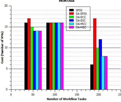
From Fig. 4, we simulated the execution of the Montage workflows and measured the execution costs in VMs number. We note that regardless of the size of the workflow, our policies give good results by reducing the number of VMs. Especially for large workflows whose size is 200 tasks; we note that the DA-MCC and DA-MCS policies use only 08 virtual machines. This result depends on the CPM matrix data and proves that there is not a better distance measure. The distance used depends on the data to be analyzed.
Fig. 4. Impact of the MONTAGE workflow on the cost.
the workflows whose size is 200 tasks. Those policies use “single” agglomeration method coupled with the Euclidian/Complete metric to measure the distances and distributes the tasks between virtual machines so that the distance between the VMs is as minimal as possible. This will naturally involve grouping highly dependent tasks into the same virtual machines (cluster) and therefore reducing file transfer between machines to a minimum.
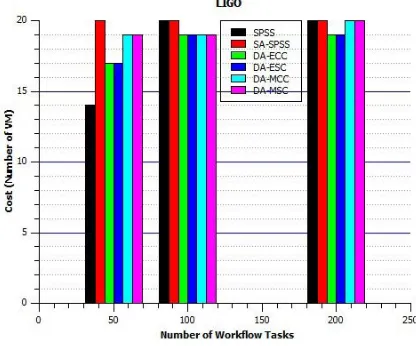
Fig. 5. Impact of the LIGO workflow on the cost.
By comparing Fig. 4 and 5, we note that the Montage workflows allocate fewer resources compared to the LIGO workflow. This confirms the information in Table II: LIGO is data-aware workflows, and Montage is processing-aware workflows. Therefore, the application of a scheduling algorithm depends on the type of the workflow.
In [45] we have several types of scientific workflows, namely, data-aware workflows, processing-aware workflows, memory-aware workflows, etc. Through the two graphs, we note that the SPSS policy gives in some cases good results. These results do not reflect reality because this policy does not support the data transfer time. Hence the importance of using a scheduling algorithm that is specific to the type of workflow [46, 47].
B. Experiment 2: Impact of the Workflow Type on the Total Data
Transfer Time
From Fig. 6, we simulated the execution of the Montage workflows and measured the total data transfer time (TDTT). We note that regardless of the size of the workflow, our policies give good results. For example, for large workflows whose size is 200 tasks, we note that the DA-MCC policy completes the total data transfer of the workflow in 456 seconds. This result reinforces our supposition of previous experience according to which cost and TDTT depend on the data we are analyzing, namely the CPM matrix. Therefore, the distance used affects the execution time and depends on the data to be analyzed.
From Fig. 7, we simulated the execution of LIGO workflows and measured the total data transfer time. We note that regardless of the size of the workflow, our policies work well. We note that our policies give good results. In particular, the DA-MCC policy that terminates the total data transfer of workflows whose size is 200 tasks at 201 seconds. This result reinforces our previous supposition in which the choice of an agglomeration method has a direct impact on the workflow scheduling. In this case, the “Complete” agglomeration method gives good results. In addition to the previous section, the choice of an agglomeration method also depends on the analyzed data, namely the CPM matrix.
Fig. 6. Impact of the MONTAGE workflow on the total data transfer time.
Fig. 7. Impact of the LIGO workflow on the total data transfer time.
From Fig. 6 and 7, we note that the Montage workflows has larger TDTT than the LIGO workflows. This has a relationship with the result of the previous simulation (Experiment 1), in which we noticed that the Montage workflow allocates fewer resources; unlike the LIGO workflow that allocates more resources which implies faster execution. For example, for the Montage workflow of 200 tasks, with the policy DA-MCC, it allocates 8 virtual machines and takes 456 seconds of TDTT. For the LIGO workflow of 200 tasks, with the same policy, it allocates 20 virtual machines and takes 201 seconds of TDTT.
Through Fig. 6 and 7, we note that the SA-SPSS policy gives in most cases bad results compared to our policies. The SA-SPSS workflow tasks scheduling is based on a network congestion subsystem that allows prediction of file transfer times.
The predicted duration time will be included in the overall task time. However, this subsystem does not take into consideration the dynamic and unpredictable nature of the underlying network.
C. Experiment 3: Impact of the Workflow Type on the Standard
Deviation
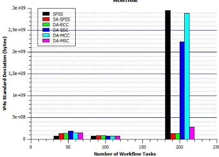
Fig. 8. Impact of the MONTAGE workflow on the standard deviation.
Fig. 9. Impact of the LIGO workflow on the standard deviation.
Unlike SA-SPSS policy that uses a subsystem allowing it to make dynamic scheduling with respect to network congestion.
Comparing Fig. 8 and 9 together, we note that the LIGO workflow generates a reduced standard deviation compared to the Montage workflow. This is because the Montage is processing-aware workflow and the LIGO is data-aware workflow. Through the two graphs, we also note that our policies give good results on LIGO workflow, which proves that our policies are better suited for data-driven workflows.
VIII. Conclusion
Cloud computing has gained popularity for the deployment and execution of workflow applications. Often, tasks and data workflow applications are distributed across cloud data centers on a global scale. So, workflow tasks need to be scheduled based on the data layout in the cloud. Since the resources obtained in the cloud are not free of charge, any proposed scheduling policy must respect the budget of the workflow.
In this paper, an approach was proposed to reduce the virtual machines costs in Cloud Computing. The objective of this work is to provide a scheduling strategy with low costs in cloud computing environment. In our strategy, the amount of global data movement can be reduced, which can decrease the inter-VMs communications rate and improve, therefore, the workflow makespan and network devices in the cloud. Our strategy model was built, based on the principles of communication efficiency-aware scheduling.
In this work a clustering approach was proposed, that could improve the use of resource efficiency and decrease virtual resources consumption during the workflow scheduling. Experiment results demonstrated that
the proposed scheduling method could simultaneously decrease virtual resources consumption and workflow makespan.
However, some of our policies have given us unexpected results, such as policies based on the “complete” agglomeration method. We then did extensive research and found that these results have a relationship with the data to be analyzed [48]; in our case, it is the structure of the
CPM matrix. In [49] we found that there are several types of data, namely, Interval-Scaled data, Dissimilarities, Similarities, Binary data, Nominal, Ordinal, Ratio data, Mixed data. Typically, before applying a distance measure or an agglomeration method, we first need to understand the data type of the CPM matrix. As future work, we will explore the field of data mining and classification to understand and define the data type in the CPM matrix and apply the right distance measure and the right agglomeration method.
In section V.B, we found that 17 clustering quality indexes do not match the CPM matrix data. As a perspective, we will try to understand the reasons why these indexes tend to infinity, and if possible to find a solution to standardize or normalize the data of the CPM matrices.
Conditional probability is one of the disciplines of probability theory. In this work, we automated the scheduling of a workflow by modeling the relationships between the tasks of a workflow with the concept of the conditional probability. As future work, we will implement our approach in machine learning. Machine learning is one of the domains of artificial intelligence which is based on statistics. This discipline is strong about modeling NP problems [50].
References
[1] O. Achbarou, M. A. E. kiram, and S. E. Bouanani, “Securing cloud computing from different attacks using intrusion detection systems,” International Journal of Interactive Multimedia and Artificial Intelligence, vol. 4, no. 3, pp. 61–64, 2017.
[2] R. J. Sethi and Y. Gil, “Scientific workflows in data analysis: Bridging expertise across multiple domains,” Future Generation Computer Systems, vol. 75, no. Supplement C, pp. 256 – 270, 2017.
[3] D. Talia, P. Trunfio, and F. Marozzo, “Chapter 3 - models and techniques for cloud-based data analysis,” in Data Analysis in the Cloud, ser. Computer Science Reviews and Trends, D. Talia, P. Trunfio, and F. Marozzo, Eds. Elsevier, 2016, pp. 45–76.
[4] “Amazon Simple Workflow Service (SWF),” https://aws.amazon.com/ swf, accessed: 2017-10-29.
[5] R. Khorsand, F. Safi-Esfahani, N. Nematbakhsh, and M. Mohsenzade, “Taxonomy of workflow partitioning problems and methods in distributed environments,” Journal of Systems and Software, vol. 132, pp. 253–271, 2017.
[6] M. R. Garey and D. S. Johnson, Computers and Intractability; A Guide to the Theory of NP-Completeness. New York, NY, USA: W. H. Freeman & Co., 1990.
[7] E. N. Alkhanak, S. P. Lee, R. Rezaei, and R. M. Parizi, “Cost optimization approaches for scientific workflow scheduling in cloud and grid computing: A review, classifications, and open issues,” Journal of Systems and Software, vol. 113, pp. 1–26, 2016.
[8] F. Wu, Q. Wu, and Y. Tan, “Workflow scheduling in cloud: a survey,” The Journal of Supercomputing, vol. 71, no. 9, pp. 3373–3418, 2015.
[9] N. M. Ndiaye, P. Sens, and O. Thiare, “Performance comparison of hierarchical checkpoint protocols grid computing,” International Journal of Interactive Multimedia and Artificial Intelligence, vol. 1, no. 5, pp. 46–53, 2012.
[10] L. Zeng, B. Veeravalli, and A. Y. Zomaya, “An integrated task computation and data management scheduling strategy for workflow applications in cloud environments,” Journal of Network and Computer Applications, vol. 50, pp. 39–48, 2015.
[11] W. T. M. Jr., P. J. Schweitzer, and T. W. White, “Problem decomposition and data reorganization by a clustering technique,” Operations Research, vol. 20, no. 5, pp. 993–1009, 1972.
in 9th Workshop on Many-Task Computing on Clouds, Grids, and Supercomputers (MTAGS2016). IEEE Computer Society, 2016, pp. 20– 25.
[13] E. I. Djebbar, G. Belalem, and M. Benadda, “Task scheduling strategy based on data replication in scientific cloud workflows,” Multiagent and Grid Systems, vol. 12, no. 1, pp. 55–67, 2016.
[14] L. Zhao, Y. Ren, and K. Sakurai, “Reliable workflow scheduling with less resource redundancy,” Parallel Computing, vol. 39, no. 10, pp. 567–585, 2013.
[15] X. Wang, C. S. Yeo, R. Buyya, and J. Su, “Optimizing the makespan and reliability for workflow applications with reputation and a look-ahead genetic algorithm,” Future Generation Computer Systems, vol. 27, no. 8, pp. 1124–1134, 2011.
[16] R. Bagheri and M. Jahanshahi, “Scheduling workflow applications on the heterogeneous cloud resources,” Indian Journal of Science and Technology, vol. 8, no. 12, 2015.
[17] “Amazon AWS service limits,” http://docs.aws.amazon.com/general/ latest/gr/aws service limits.html, accessed: 2017-10-29.
[18] “Amazon EC2 on-demand instances limits,” https://aws.amazon.com/ec2/ faqs/#How many instances can I run in Amazon EC2, accessed: 2017-10-29.
[19] “Amazon EC2 reserved instance limits,” http://docs.aws.amazon. com/ AWSEC2/latest/UserGuide/ec2-reserved-instances.html#ri-limits, accessed: 2017-10-29.
[20] V. Singh, I. Gupta, and P. K. Jana, “A novel cost-efficient approach for deadline-constrained workflow scheduling by dynamic provisioning of resources,” Future Generation Computer Systems, vol. 79, pp. 95–110, 2018.
[21] M. Malawski, G. Juve, E. Deelman, and J. Nabrzyski, “Algorithms for cost and deadline-constrained provisioning for scientific workflow ensembles in iaas clouds,” Future Generation Computer Systems, vol. 48, pp. 1–18, 2015, special Section: Business and Industry Specific Cloud.
[22] R. N. Calheiros, R. Ranjan, A. Beloglazov, C. A. F. D. Rose, and R. Buyya, “Cloudsim: A toolkit for modeling and simulation of cloud computing environments and evaluation of resource provisioning algorithms,” Software: Practice and Experience, vol. 41, no. 1, pp. 23–50, 2011.
[23] C. Wu and R. Buyya, “Chapter 12 - cloud storage basics,” in Cloud Data Centers and Cost Modeling. Morgan Kaufmann, 2015, pp. 425–495.
[24] L. Torgo, Data mining with R: learning with case studies. CRC Press, 2016.
[25] M. Charrad, N. Ghazzali, V. Boiteau, and A. Niknafs, “Nbclust: An R package for determining the relevant number of clusters in a data set,” Journal of Statistical Software, vol. 61, no. 6, pp. 1–36, 2014.
[26] W. J. Krzanowski and Y. T. Lai, “A criterion for determining the number of groups in a data set using sum-of-squares clustering,” Biometrics, vol. 44, no. 1, pp. 23–34, 1988.
[27] T. Cali´nski and J. Harabasz, “A dendrite method for cluster analysis,” Communications in Statistics-Simulation and Computation, vol. 3, no. 1, pp. 1–27, 1974.
[28] J. A. Hartigan, Clustering Algorithms, 99th ed. John Wiley & Sons, Inc., 1975.
[29] J. O. McClain and V. R. Rao, “Clustsiz: A program to test of the quality of clustering a set of objects,” Journal of Marketing Research, vol. 12, no. 4, pp. 456–460, 1975.
[30] F. B. Baker and L. J. Hubert, “Measuring the power of hierarchical cluster analysis,” Journal of the American Statistical Association, vol. 70, no. 349, pp. 31–38, 1975.
[31] F. J. Rohlf, “Methods of comparing classifications,” Annual Review of Ecology and Systematics, vol. 5, pp. 101–113, 1974.
[32] G. W. Milligan, “A review of monte carlo tests of cluster analysis,” Multivariate Behavioral Research, vol. 16, no. 3, pp. 379–407, 1981.
[33] J. C. Dunn, “Well-separated clusters and optimal fuzzy partitions,” Journal of Cybernetics, vol. 4, no. 1, pp. 95–104, 1974.
[34] M. Halkidi, M. Vazirgiannis, and Y. Batistakis, Quality Scheme Assessment in the Clustering Process. Springer Berlin Heidelberg, 2000, pp. 265–276.
[35] M. Halkidi and M. Vazirgiannis, “Clustering validity assessment: Finding the optimal partitioning of a data set,” in Proceedings of the 2001 IEEE International Conference on Data Mining, 29 November - 2 December 2001, San Jose, California, USA, 2001, pp. 187–194.
[36] L. J. Hubert and J. R. Levin, “A general statistical framework for assessing
categorical clustering in free recall,” Psychological Bulletin, vol. 83, no. 6, pp. 1072–1080, 1976.
[37] P. J. Rousseeuw, “Silhouettes: A graphical aid to the interpretation and validation of cluster analysis,” Journal of Computational and Applied Mathematics, vol. 20, no. Supplement C, pp. 53–65, 1987.
[38] G. H. Ball and D. J. Hall, “Isodata, a novel method of data analysis and pattern classification,” Stanford research inst Menlo Park CA, Tech. Rep., 1965.
[39] G. W. Milligan, “An examination of the effect of six types of error perturbation on fifteen clustering algorithms,” Psychometrika, vol. 45, no. 3, pp. 325–342, 1980.
[40] F. Z. Filali and B. Yagoubi, “Classifying and filtering users by similarity measures for trust management in cloud environment,” Scalable Computing: Practice and Experience, vol. 16, no. 3, pp. 289–302, 2015.
[41] R. F. da Silva, W. Chen, G. Juve, K. Vahi, and E. Deelman, “Community resources for enabling research in distributed scientific workflows,” in eScience. IEEE Computer Society, 2014, pp. 177–184.
[42] A. C. Zhou, B. He, and S. Ibrahim, “Chapter 18 - escience and big data workflows in clouds: A taxonomy and survey,” in Big Data. Morgan Kaufmann, 2016, pp. 431–455.
[43] M. A. Rodriguez and R. Buyya, “Chapter 18 - scientific workflow management system for clouds,” in Software Architecture for Big Data and the Cloud. Boston: Morgan Kaufmann, 2017, pp. 367–387.
[44] P. Bryk, M. Malawski, G. Juve, and E. Deelman, “Storage-aware algorithms for scheduling of workflow ensembles in clouds,” Journal of Grid Computing, vol. 14, no. 2, pp. 359–378, 2016.
[45] G. Juve, A. Chervenak, E. Deelman, S. Bharathi, G. Mehta, and K. Vahi, “Characterizing and profiling scientific workflows,” Future Generation Computer Systems, vol. 29, no. 3, pp. 682–692, 2013, special Section: Recent Developments in High Performance Computing and Security.
[46] M. Masdari, S. ValiKardan, Z. Shahi, and S. I. Azar, “Towards workflow scheduling in cloud computing: A comprehensive analysis,” Journal of Network and Computer Applications, vol. 66, no. Supplement C, pp. 64–82, 2016.
[47] J. Sahni and D. P. Vidyarthi, “Workflow-and-platform aware task clustering for scientific workflow execution in cloud environment,” Future Generation Computer Systems, vol. 64, no. Supplement C, pp. 61–74, 2016.
[48] C. C. Aggarwal, Ed., Data Classification: Algorithms and Applications. CRC Press, 2014.
[49] L. Kaufman and P. J. Rousseeuw, Finding Groups in Data: an Introduction to Cluster Analysis. Wiley, 1990.
[50] S. I. Serengil and A. Ozpinar, “Workforce optimization for bank operation centers: A machine learning approach,” International Journal of Interactive Multimedia and Artificial Intelligence, vol. 4, no. 6, pp. 81–87, 2017.
Sid Ahmed Makhlouf
Ph.D. candidate in the University of Oran1 Ahmed Ben Bella (Algeria). His main research interests include Distributed System, Cluster, Grid & Cloud Computing, Load Balancing, Task & Workflow Scheduling, and Machine Learning.
Belabbas Yagoubi