Unsupervised Domain Adaptation Based on Source-Guided Discrepancy

The Thirty-Third AAAI Conference on Artificial Intelligence (AAAI-19)

Unsupervised Domain Adaptation Based on Source-Guided Discrepancy

Seiichi Kuroki,

Nontawat Charoenphakdee,

Han Bao,

Junya Honda,

Issei Sato,

Masashi Sugiyama

†_{The University of Tokyo, Tokyo, Japan}

‡_{RIKEN, Tokyo, Japan}

Abstract

Unsupervised domain adaptation is the problem setting where data generating distributions in the source and tar-get domains are different and labels in the tartar-get domain are unavailable. An important question in unsupervised do-main adaptation is how to measure the difference between the source and target domains. Existing discrepancy measures for unsupervised domain adaptation either require high computa-tion costs or have no theoretical guarantee. To mitigate these problems, this paper proposes a novel discrepancy measure calledsource-guided discrepancy (S-disc), which exploits la-bels in the source domain unlike the existing ones. As a con-sequence, S-disc can be computed efficiently with a finite-sample convergence guarantee. In addition, it is shown that S-disc can provide a tighter generalization error bound than the one based on an existing discrepancy measure. Finally, ex-perimental results demonstrate the advantages of S-disc over the existing discrepancy measures.

Introduction

In the conventional supervised learning framework, we of-ten assume that the training and test distributions are the same. However, this assumption may not hold in many prac-tical applications such as natural language processing (Glo-rot, Bordes, and Bengio 2011), speech recognition (Sun et al. 2017), and computer vision (Saito, Ushiku, and Harada 2017). For instance, a personalized spam filter can be trained from the emails of all available users, but the training data may not represent the emails of the target user. Such scenarios can be formulated in the framework of domain adaptation, which has been studied extensively (Ben-David et al. 2007; Mansour, Mohri, and Rostamizadeh 2009a; Zhang, Zhang, and Ye 2012; Pan and Yang 2010; Sugiyama and Kawanabe 2012). An important challenge in domain adaptation is to find a classifier for a label-scarce target do-main by exploiting a label-rich source dodo-main. In particular, there are cases where we only have access to labeled data from the source domain and unlabeled data from the tar-get domain, because annotating labels in the tartar-get domain is often time-consuming and expensive (Saito et al. 2018).

∗

A longer version of this paper is available in Kuroki et al. (2018).

Copyright c2019, Association for the Advancement of Artificial Intelligence (www.aaai.org). All rights reserved.

This problem setting is called unsupervised domain adap-tation(Ben-David et al. 2007), which is our interest in this paper.

Since domain adaptation cannot be performed effectively if the source and target domains are too different, an im-portant topic to be addressed is how to measure the dif-ference, or discrepancy, between the two domains. Many discrepancy measures have been used in previous studies such as the maximum mean discrepancy (Huang et al. 2007), Kullback-Leibler divergence (Sugiyama et al. 2008), R´enyi divergence (Mansour, Mohri, and Rostamizadeh 2009b), and Wasserstein distance (Courty et al. 2017).

Apart from the discrepancy measures described above, Ben-David et al. (2007) proposed a discrepancy measure for binary classification that explicitly takes a hypothesis class into account. They showed that their discrepancy measure leads to a tighter generalization error bound than the L1

distance, which does not use information of the hypothesis class. Following this line of research, Mansour, Mohri, and Rostamizadeh (2009a) generalized the discrepancy mea-sure of Ben-David et al. (2007) to arbitrary loss functions, and Germain et al. (2013) provided a PAC-Bayesian anal-ysis based on the average disagreement of a set of hy-potheses. These results provided a theoretical foundation for various applications of domain adaptation based on es-timation of source-target discrepancy, including sentiment analysis (Glorot, Bordes, and Bengio 2011), source selec-tion (Bhatt, Rajkumar, and Roy 2016), and multi-source domain adaptation (Zhao et al. 2017). However, their dis-crepancy measure considers the worst pair of hypotheses to bound the maximum gap in the loss between the domains, which may lead to a loose generalization error bound and expensive computation costs. Zhang, Zhang, and Ye (2012) and Mohri and Medina (2012) analyzed another discrepancy measure with a generalization error bound. Nevertheless, this discrepancy measure cannot be computed without la-bels in the target domain and therefore is not suitable for unsupervised domain adaptation.

and Rostamizadeh (2009a). Furthermore, we provide an es-timator of S-disc for binary classification that can be com-puted efficiently. We also establish consistency and analyze the convergence rate of the proposed S-disc estimator.

Our main contributions are as follows.

• We propose a novel discrepancy measure called source-guided discrepancy (S-disc), which uses labels in the source domain to measure the difference between the two domains for unsupervised domain adaptation (Defi-nition 2).

• We propose an efficient algorithm for estimating S-disc for the 0-1 loss (Algorithm 1).

• We show the consistency and elucidate the convergence rate of the estimator of S-disc (Theorem 4).

• We derive a generalization error bound in the target do-main based on S-disc (Theorem 7), which is tighter than the existing bound provided by Mansour, Mohri, and Ros-tamizadeh (2009a). In addition, we derive a generalization error bound for a finite-sample case (Theorem 8). • We demonstrate the effectiveness of S-disc for

unsuper-vised domain adaptation in experiments.

Problem Setting and Notation

In this section, we formulate the unsupervised domain adap-tation problem. Let_Xbe the input space and_Ybe the output space, which is_{+1,₋1_}in binary classification. We define a domain as a pair (PD, fD), wherePD is an input

distri-bution on_X andfD:X → Y is a labeling function. In

do-main adaptation, we denote the source dodo-main and the target domain as (PS,fS) and (PT,fT), respectively. Unlike

con-ventional supervised learning, we focus on the case where (PT,fT) differs from (PS,fS). In unsupervised domain

adap-tation, we are given the following data:

• Unlabeled data in the target domain:_T =_{xT i}

nT i=1.

• Labeled data in the source domain:_S =_{(xS_j, yS_j)_}nS j=1.

For simplicity, we denote the input features from the source domain_{xS_j}nS

j=1asSXand the empirical distribution

corre-sponding toPT(resp.PS) asPbT(resp.PbS).

We denote a loss function `: _{R × R → R}+. For

example, the 0-1 loss is given as `01(y, y0) = (1 −

sign(yy0))/2. The expected loss for functionsh, h0 :_{X →}

Rand distribution PD over X is denoted byR`D(h, h0) =

Ex∼PD[`(h(x), h

0_{(x))]. We also denote an empirical risk as}

b R`

D(h, h0) =Ex∼PbD[`(h(x), h

0_{(x))]. In addition, we define}

the true risk minimizer and the empirical risk minimizer in a certain domain (PD,fD) in a hypothesis classHash∗D =

arg min_h∈HR`

D(h, fD)andbhD= arg minh∈HRb`_D(h, fD),

respectively. Here, note that the risk minimizer h∗ D is not

necessarily equal to the labeling functionfDas we consider

a restricted hypothesis class.

The goal in domain adaptation is to find a hypothesish out of a hypothesis class_Hso that it gives as small expected loss as possible in the target domain defined by

R`T(h, fT) =Ex∼PT[`(h(x), fT(x))].

Related Work

In unsupervised domain adaptation, it is essential to mea-sure the difference between the source and target domains, because it might degrade the performance to use data col-lected from a source domain that is far from the target do-main (Pan and Yang 2010). Since we cannot access labels from the target domain, it is impossible to measure the dif-ference between the two domains on the basis of theoutput space. One way is to measure the difference between proba-bility distributions in terms of theinput space.

We will review such discrepancy measures in this section. First, we introduce the discrepancy measure proposed by Mansour, Mohri, and Rostamizadeh (2009a), which is de-fined as

disc`_H(PT, PS) = sup h,h0_∈H

R`T(h, h0)−R`S(h, h0) . (1)

We call this discrepancy measure_X-disc as it does not re-quire labels from the source domain but input features. Note that_X-disc takes the hypothesis class_Hinto account.

Mansour, Mohri, and Rostamizadeh (2009a) showed that the following inequalities hold for anyh, h0_{∈ H}:

R`<sub>T</sub>(h, h0)−R`_S(h, h0) ≤disc

`

H(PT, PS)

≤M_·L1(PT, PS),

whereM > 0is a constant andL1(·,·)is theL1distance

over distributions. Therefore, a tighter bound for the differ-ence in the expected loss between the two domains can be obtained by considering a hypothesis class_H. However, a drawback of _X-disc is that it considers the worst pair of hypotheses as can be seen from (1). This may lead to a loose generalization error bound as we will show later, and also an intractable computation cost for empirical estima-tion. Ben-David et al. (2007) provided a computationally ef-ficient proxy of_X-disc for the 0-1 loss defined as follows:

dH(PT, PS) = sup h∈H R

`01

T (h,1)−R `01

S (h,1) .

AlthoughdHcan be computed efficiently, there is no

learn-ing guarantee.

There is another variant of_X-disc called the generalized discrepancy (Cortes, Mohri, and Medina 2015). However, the theoretical analysis therein is only applicable to the re-gression task and not suitable for binary classification unlike the analysis for_X-disc.

Another discrepancy measure_Y-disc which also takes_H into account is as follows:

Y-disc`_H(PT, PS) = sup h∈H|

R`<sub>T</sub>(h, fT)−RS`(h, fS)|.

While_Y-disc has been proposed to provide a tighter gener-alization error bound than_X-disc (Mohri and Medina 2012; Zhang, Zhang, and Ye 2012), it requires the labeling func-tionfTin the test domain which cannot be estimated in

un-supervised domain adaptation in general.

limitations of the existing discrepancy measures. Later, we will show that S-disc can provide a tighter generalization bound and can be computed efficiently compared with the existing measures.

We define S-disc as follows, which is obtained by fixing h0in the definition (1) of_X-disc to the true risk minimizer h∗_S= arg min_h∈HR`

S(h, fS)in the source domain.

Definition 1(Source-guided discrepancy). Let_Hbe a hy-pothesis class and let`: _{R×R →R}+ be a loss function.

S-disc between two distributionsPD1 andPD2is defined as

ς_H`(PD1, PD2) = sup h∈H R

` D1(h, h

∗ S)−R

` D2(h, h

∗ S)

. (2)

S-disc satisfies the triangular inequality, i.e., ς`

H(PD1, PD2) ≤ ς `

H(PD1, PD3) + ς `

H(PD3, PD2), and is symmetric, i.e.,ς`

H(PD1, PD2) = ς `

H(PD2, PD1). How-ever, in general, S-disc is not a distance as we may have ς`

H(PD1, PD2) = 0for somePD1 6=PD2.

S-disc has the following three advantages over existing discrepancy measures. First, the computation cost of S-disc is low since we do not need to consider a pair of hypotheses unlike_X-disc as we can see from (1) and (2). Second, S-disc leads to a tighter bound as discussed below. Mansour, Mohri, and Rostamizadeh (2009a) derived a generalization error bound by bounding the differenceR`<sub>T</sub>(h, h∗<sub>S</sub>)−R`_S(h, h∗_S)

with_X-disc. On the other hand, for anyh_{∈ H}, it is easy to see that from the definition of S-disc

R`T(h, h∗S)−R`S(h, h∗S)

≤ς_H`(PT, PS)

≤disc`_H(PT, PS), (3)

which implies that S-disc gives a tighter generalization error bound than_X-disc. Third, sinceh∗_Sis estimated by labeled data from the source domain, we can compute S-disc with-out labels from the target domain unlike_Y-disc. For these reasons, S-disc is more suitable for unsupervised domain adaptation than the existing discrepancy measures. A com-parison of S-disc with the existing discrepancy measures is summarized in Table 1.

S-disc Estimation for the 0-1 Loss

Here we consider the task of binary classification with the 0-1 loss, where the output space_Yis_{+1,₋1_}. The follow-ing theorem states that S-disc estimation can be reduced to a cost-sensitive classification problem. We consider a sym-metric hypothesis class_H, which is closed under negation, i.e., for anyh_{∈ H},₋his contained in_H.

Theorem 2. For the 0-1 loss and a symmetric hypothesis class_H, the following equality holds:

ς`01

H (PbT,PbS) = 1−min

h∈HJ`01(h),

whereJ`(h)is defined as

J`(h) =

1

nS nS X

j=1

`(h(xS_j), h∗_S(xS_j))

+ 1

nT nT X

i=1

`(h(xT_i),₋h∗_S(xT_i)).

Algorithm 1:S-disc Estimation for the 0-1 Loss

Input:labeled source data_S, unlabeled target data_T, surrogate loss`sur, hypothesis classH. Output:ς<sub>H</sub>`(PbT,PbS).

Source learning:

Learn a classifierbhSusing labeled source dataSX.

Pseudo labeling:

• Se={(x,sign◦bhS(x))|x∈ SX},

• Te ={(x,−sign◦bhS(x))|x∈ T }.

Cost sensitive learning from pseudo labeled data

Learn another classifier h00 _{∈ H}using SeandTe to minimize the surrogate cost-sensitive riskJ`sur.

returnς`

H(PbT,PbS)=1−J`01(h

00_).

The proof of Theorem 2 is given in Kuroki et al. (2018). Note that the minimization ofJ`01(h)corresponds to em-pirical risk minimization for_S∗ = _{(x, h_S∗(x))_| x_{∈ S}X}

and_T∗ = _{(x,₋h∗_S(x)) _| x_{∈ T }}. Therefore, Theorem 2 naturally suggests a three-step algorithm illustrated in Al-gorithm 1, whereh∗_Sis replaced withbhS. This allows us to

compute S-disc by minimizer h00 of the cost-sensitive risk J`01(h), which weights the pseudo-labeled data Seand Te with costs1/nSand1/nT, respectively.

Since minimization of the 0-1 loss is computationally hard (Ben-David, Eiron, and Long 2003; Feldman et al. 2012), we use a surrogate loss such as the hinge loss `hinge(y, y0) = max(0,1 − yy0) (Bartlett, Jordan, and McAuliffe 2006). Note that the 0-1 loss is used for cal-culating S-disc in the final step, i.e., 1 <sub>−</sub>J`01(h

00_{), while}

a surrogate loss is only used to train a classifier. Hinge loss minimization with the sequential minimal optimization (SMO) algorithm requiresO((nT+nS)3)for the entire

al-gorithm (Platt 1999). This low computation cost has a big advantage over_X-disc (see Table 1).

Theoretical Analysis

In this section, we show that S-disc can be estimated from fi-nite data with the consistency guarantee. After that, we show that our proposed S-disc is useful for deriving a tighter gen-eralization error bound than _X-disc. To derive theoretical results, theRademacher complexityis used, which captures the complexity of a set of functions by measuring the ca-pability of a hypothesis class to correlate with the random noise.

Definition 3(Rademacher complexity (Bartlett and Mendel-son 2002)). Let_Hbe a set of real-valued functions defined over a set _X. Given a sample (x1, . . . , xm) ∈ Xm inde-pendently and identically drawn from a distribution µ, the Rademacher complexity of_His defined as

Rµ,m(H) =Ex1,...,xmEσ "

sup

h∈H

1

m m X

i=1

σih(xi) #

,

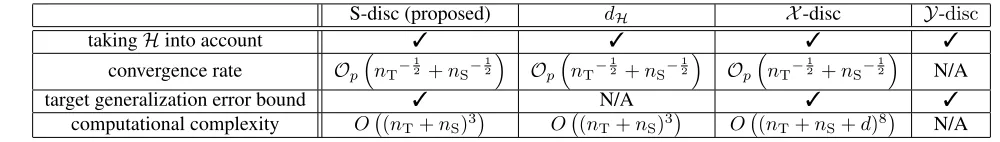
Table 1: Comparison of S-disc with the existing discrepancy measures for unsupervised domain adaptation in binary classifica-tion. We assume the hypothesis class_Hsatisfies (4). We consider the hinge loss for S-disc,_X-disc, anddH. The computational

complexity of S-disc anddHare based on the empirical hinge loss minimization, which is solved with the kernel support vector

machine by the SMO algorithm (Platt 1999). The computational complexity of_X-disc is that based on SDP relaxation by the ellipsoid method (Bubeck 2015) given in Kuroki et al. (2018)._Y-discis not computable with unlabeled target data.

S-disc (proposed) dH X-disc Y-disc

taking_Hinto account _{3 3 3 3}

convergence rate _Op

nT−

1 2 +n_S−

1 2

Op

nT−

1 2 +n_S−

1 2

Op

nT−

1 2 +n_S−

1 2

N/A

target generalization error bound 3 N/A 3 3

computational complexity O (nT+nS)3

O (nT+nS)3

O (nT+nS+d)8

N/A

which are mutually independent uniform random variables taking values in_{+1,₋1_}.

Hereafter, we use the following notation: • H ⊗ H:=_{x_7→h(x)_·h0(x)_|h, h0_{∈ H}}, • `<sub>◦</sub>(<sub>H ⊗ H</sub>) :=<sub>{</sub>x<sub>7→</sub>`(h(x), h0(x))_|h, h0_{∈ H}}.

Consistency of S-disc

In this section, we show the estimatorς`

H(PbT,PbS)converges

to the true S-discς`

H(PT, PS)as the numbers of samplesnT

andnSincrease. The following theorem gives the deviation

of the empirical S-disc estimator, which is a general result that does not depend on the specific choice of the loss`and the hypothesis class_H.

Theorem 4. Assume the loss function `is bounded from above by M > 0. For anyδ _∈ (0,1), with probability at least1₋δ,

ς

`

H(PbT,PbS)−ςH`(PT, PS)

≤2RPT,nT(`◦(H ⊗ H)) + 2RPS,nS(`◦(H ⊗ H))

+M s

log4_δ 2nT

+M s

log4_δ 2nS

.

The proof of this theorem is given in Kuroki et al. (2018). Theorem 4 guarantees the consistency ofς`

H(PbT,PbS)

un-der the condition thatRPT,nT(`◦(H ⊗ H))andRPS,nS(`◦

(_{H ⊗ H}))are well-controlled.

To derive a specific convergence rate, we consider an as-sumption given by

RPT,nT(H ⊗ H)≤

CH⊗H

√_n

T

, RPS,nS(H ⊗ H)≤

CH⊗H

√_n

S

,

(4)

for some constantCH⊗H>0depending only on the

hypoth-esis class_H. Lemma 5 below shows that this assumption is naturally satisfied in the linear-in-parameter model.

Lemma 5. Let _Hbe the linear-in-parameter model class, i.e.,_H:=_{x_7→w>φ(x)_|w_∈Rd, kwk2 ≤Λ}for fixed

basis functionsφ:_{X →}Rdsatisfyingkφk∞ ≤Dφ. Then, for any distributionµover_X andm_∈N,

Rµ,m(H ⊗ H)≤

Λ2_D2 φ √_m .

The proof of Lemma 5 is given in Kuroki et al. (2018). Subsequently, we derive the convergence rate bound for the 0-1 loss.

Corollary 6. When we consider` = `01, it holds for any

δ_∈(0,1)that, with probability at least1₋δ,

ς

`

H(PbT,PbS)−ςH`(PT, PS)

≤ C√H⊗H_n

T

+C_√H⊗H

nS

+

s

log4_δ 2nT

+

s

log4_δ 2nS

under the assumption in (4).

Proof. It simply follows from Theorem 4, the assumption in (4), and the factRµ,k(`01◦(H ⊗ H)) = 12Rµ,k(H ⊗ H) for any distributionµandk >0(Mohri, Rostamizadeh, and Talwalkar 2012, Lemma 3.1).

From this corollary, we see that the empirical S-disc has the consistency with convergence rate _Op(nT−1/2 +

nS−1/2)under a mild condition.

Generalization Error Bound

In the previous section, we showed that S-discς_H`(PT, PS)

can be estimated byς_H`(PbT,PbS). In this section, we give two

bounds on the generalization errorR`

T(h, fT)for the target

domain in terms ofς`

H(PT, PS)orςH`(PbT,PbS).

The first bound shows the relationship between target risk R`

T(h, fT)and source riskR`S(h, h∗S).

Theorem 7. Assume that`obeys the triangular inequality, i.e.,`(u, v)_≤`(u, w) +`(w, v), _∀u, v, w _∈R,such as the 0-1 loss. Then, for any hypothesish_{∈ H},

R`<sub>T</sub>(h, fT)−R`T(h ∗ T, fT)

≤R`<sub>S</sub>(h, h∗<sub>S</sub>) +R`_T(h_S∗, h∗_T) +ς_H`(PT, PS). (5) Proof. Since

R_T`(h, fT)≤RT`(h, h∗S) +R `

T(h∗S, h∗T) +R `

T(h∗T, fT)

holds from the triangular inequality, we have

R`<sub>T</sub>(h, fT)−R`T(h∗T, fT)

≤R`T(h, h∗S) +RT`(h∗S, h∗T)

≤R`<sub>S</sub>(h, h∗<sub>S</sub>) +R`_T(h_S∗, h∗_T) +ς_H`(PT, PS),

The LHS of (5) represents the regret arising from the use of hypothesis h instead of h∗_T in the target domain. The-orem 7 shows that the regret R`

T(h, fT)−R`T(h ∗ T, fT) is

bounded by three terms: (i) the expected loss with respect to h∗_Sin the source domain, (ii) the difference betweenh∗_Tand h∗_Sin the target domain, and (iii) S-disc betweenPTandPS.

Note that if the source and target domains are sufficiently close, we can expect the second termR`<sub>T</sub>(h∗<sub>S</sub>, h∗<sub>T</sub>)and the third termς<sub>H</sub>`(PT, PS)to be small. This fact indicates that

for an appropriate source domain, minimization of estima-tion errorR`_S(h, h∗_S)in the source domain leads to a better generalization in the target domain.

We can see an advantage of the generalization error bound based on S-disc through comparison with the bound based on_X-disc (Mansour, Mohri, and Rostamizadeh 2009a, The-orem 8) given by

R`<sub>T</sub>(h, fT)−R`T(h∗T, fT)

≤R`<sub>S</sub>(h, h∗<sub>S</sub>) +R<sub>T</sub>`(h_T∗, h∗_S) + disc`_H(PT, PS). (6)

The upper bound (6) using_X-disc has the same form as the upper bound (5) except for the termς_H`(PT, PS). Since

S-disc is never larger than _X-disc (see the inequality (3)), S-disc gives a tighter bound than_X-disc.

The following theorem shows the generalization error bound for the finite-sample case.

Theorem 8. When we consider`=`01, for anyh∈ Hand

δ_∈(0,1), with probability at least1₋δ,

R`<sub>T</sub>(h, fT)−R`T(h ∗ T, fT)

≤Rb`<sub>S</sub>(h, h∗<sub>S</sub>) +R`_T(h_S∗, h∗_T) +ς_H`(PbT,PbS)

+C_√H⊗H

nT

+C_√H⊗H

nS

+

s

log5_δ 2nT

+ 2

s

log5_δ 2nS

under the assumption in (4).

The proof of this theorem is given in Kuroki et al. (2018). Theorem 8 tells us that when nS, nT → ∞the

follow-ing three terms are dominatfollow-ing in the bound of the regret in the target domainR`

T(h, fT)−RT`(h∗T, fT): (i) the

em-pirical loss with respect toh∗

Sin the source domain, (ii) the

difference betweenh∗_Tandh∗_Sin the target domain, and (iii) S-disc between the two empirical distributionsς`

H(PbT,PbS).

Therefore, ifh∗_Tis sufficiently close toh∗_S, selecting a good source in terms of S-disc allows us to achieve good target generalization.

Comparison with Existing Discrepancy

Measures

In the previous section, we showed the consistency of the es-timator for S-disc and derived a generalization error bound of S-disc tighter than_X-disc. In this section, we first com-pare these theoretical guarantees of S-disc with those for the existing ones in more detail. We next discuss their compu-tation cost. This is also an important aspect when we ap-ply these discrepancy measures to sentiment analysis (Bhatt, Rajkumar, and Roy 2016), adversarial learning (Zhao et al.

2017), and computer vision (Saito et al. 2018) for source se-lection or reweighting of the source data. In fact, in these applications the discrepancy dH instead of X-disc is used

for ease of computation even thoughdH has no theoretical

guarantee on the generalization error. The results of this sec-tion are summarized in Table 1.

Convergence Rates of Discrepancy Estimators

Here we discuss the consistency and convergence rates of the estimators of discrepancy measures.

The empirical estimator of dH is consistent, and

its convergence rate is _Op(((lognT)/nT)1/2 +

((lognS)/nS)1/2) (Ben-David et al. 2010, Lemma 1).

This rate is slower than the rate _Op nT−1/2+nS−1/2

for S-disc with appropriately controlled Rademacher complexitiesRPT,nT(H)andRPS,nS(H)of the hypothesis class, such as the linear-in-parameter model (Mohri, Ros-tamizadeh, and Talwalkar 2012, Theorem 4.3). Here recall that no generalization error bound is known in terms ofdH

even thoughdHitself is consistently estimated.

On the other hand, the empirical estimator of _X-disc is shown to be consistent (Mansour, Mohri, and Ros-tamizadeh 2009a, Corollary 7) and its convergence rate is Op(nT−1/2+nS−1/2)in the case that the loss function is

`qloss, i.e.,`q(y, y0) =|y−y0|q. Thus, the derived rate is the same as S-disc whereas the requirement on the loss function is more restrictive than the one for S-disc in Theorem 8.

Note that the above difference of the theoretical guaran-tees does not come from the inherent difference of these es-timators. This is because we adopted the analysis based on the Rademacher complexity, which has not been well stud-ied in the context of unsupervised domain adaptation. This is a distribution-dependent complexity measure and less pes-simistic compared with the VC-dimension used in the previ-ous work (Ben-David et al. 2010). In fact, the known guar-antees ondHandX-disc can be improved to Propositions 9

and 10 given below.

Proposition 9. For anyδ_∈(0,1), with probability at least

1₋δ,

dH(PbT,PbS)−dH(PT, PS)

≤2RPT,nT(H) + 2RPS,nS(H) + s

2 log4_δ

nT

+

s

2 log4_δ

nS

.

Proposition 10. Assume the loss function ` is upper bounded byM > 0. For anyδ _∈ (0,1), with probability at least1₋δ,

disc

`

H(PbT,PbS)−disc`H(PT, PS)

≤2RPT,nT(`◦(H ⊗ H)) + 2RPS,nS(`◦(H ⊗ H))

+M s

log4_δ 2nT

+M s

log4_δ 2nS

.

−8 −6 −4 −2 0 2 4 6 8

x

−8 −6 −4 −2 0 2 4 6

x

S1pos

S1neg

S2pos

S2neg

Tpos

Tneg

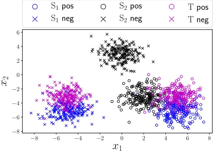
Figure 1: 2D plots of three domains.

In summary, under the mild assumptions, the conver-gence rates of the empirical estimators of dH andX-disc

are_Op nT−1/2+nS−1/2as well as S-disc.

Computational Complexity

Computation ofdH can be done by the empirical risk

min-imization (Ben-David et al. 2010, Lemma 2). The original form is given with the 0-1 loss, which can be efficiently min-imized with a surrogate loss. When the hinge loss is applied, the minimization can be carried out with the computation costO((nT+nS)3)by the SMO algorithm (Platt 1999).

On the other hand, no efficient algorithm is given for the computation of_X-disc in the classification setting.1 _{For a} fair comparison, we give a relatively efficient algorithm to compute _X-disc (1) in the classification setting with the hinge loss, based onsemidefinite relaxation. Unfortunately, the computational complexity of the relaxed algorithm is stillO((nT+nS+d)8), which is prohibitive compared with

the computation of S-disc anddH.

Experiments

In this section, we provide the experimental results that il-lustrate the failure of existing discrepancy measures and the advantage of using S-disc. We illustrate the advantage of S-disc in terms of computation time, the empirical conver-gence, and the performance on the source selection task.

Illustration

We illustrate the failure of dH, which is the well-known

proxy for_X-disc. We compared S-disc withdH in the toy

experiment.

We generated200 data points per class for each of two

1

A computation algorithm ofX-disc for the 0-1 loss is given only in the one-dimensional case (Mansour, Mohri, and Ros-tamizadeh 2009a, Section 5.2).

sourcesS1andS2and target domain as follows:

PSi(X|Y =j) =N(µ

(j)

i , I) (i= 1,2), PT(X|Y =j) =N(µ

(j) T , I),

where

µ(0)₁ = (₋5,₋5), µ(0)₂ = (0,3), µ(0)_T = (₋5,₋3), µ(1)₁ = (5,₋5), µ(1)₂ = (2,₋3), µ(1)_T = (5,₋3).

In this experiment, we used the support vector machine with a linear kernel2. For these data, we obtained the follow-ing results:

ς_H`(PbT,PbS1) = 0.27, ς `

H(PbT,PbS2) = 0.49, dH(PbT,PbS1) = 0.69, dH(PbT,PbS2) = 0.49.

These values indicate that whiledHregardsS2as the

bet-ter source, S-disc regardsS1 as the better source for target

domain.

In this example, the loss calculated on the target domain of the classifier trained onS1is 0.0 and the loss of the

clas-sifier trained onS2 is 0.49. This implies that S-disc is the

better discrepancy measure to measure the quality of source domains for a better generalization in a given target domain. Intuitively, dH is a heuristic measure based on a

classi-fier separating the source and target domains without con-sidering labels in the source domain. Once the supports of the input distributions are not highly overlapped between the source and target domains ,dHmay immediately regard that

domains are totally different from each other even if the risk minimizers are highly similar between these domains, which resulted in the failure ofdH. On the other hand, S-disc can

prevent such a problem by taking labels from the source do-main into account as illustrated in the toy experiments and justified in Theorems 7 and 8.

Comparison of Computation Time

We compared the computation time to estimate S-disc,dH,

and_X-disc. We used 2-dimensional 200 examples for both source and target domains. Each domain consists of 100 positive examples and 100 negative examples. For the com-putation of_X-disc, we used the relaxed algorithm3 shown in Kuroki et al. (2018). For bothdHand S-disc, we used the

support vector machine with a linear kernel for the compu-tation of S-disc anddH. The simulation was run on 2.8GHz

IntelR _{Core i7. The results shown in Figure 2 demonstrate} that the computation time of_X-disc is prohibitive while both S-disc anddH are feasible to compute as suggested in

Ta-ble 1.

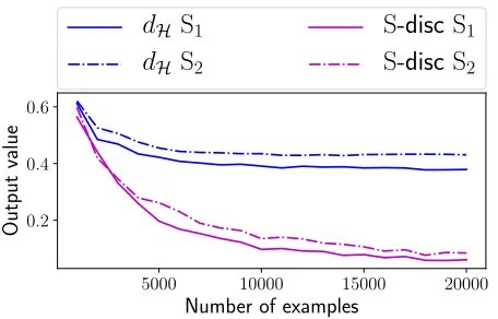
Empirical Convergence

We compared the empirical convergence of S-disc anddH

based on logistic regression implemented with scikit-learn with default parameters (Pedregosa et al. 2011). Note that

2

We used scikit-learn (Pedregosa et al. 2011) to implement it. 3

10−2 ₁₀0 ₁₀2 ₁₀4

Computation time [sec]

S-disc

dH

X-disc

Figure 2: Comparison of computation time in the log scale.

5000 10000 15000 20000

Number of examples

0.2 0.4 0.6

Output

value

d

S

d

S

S

-disc

S

S

-disc

S

Figure 3: Empirical convergence ofdHand S-disc.

X-disc is not used due to computational intractability. Here, we used MNIST (LeCun, Cortes, and Burges 2010) dataset, and considered a binary classification task to separate odd and even digits. We defined the source and target domains as follows:

• Source domainS1: MNIST,

• Source domainS2: MNIST from zero to seven,

• Target domain: MNIST.

The number of examples was ranged from_{1000, 2000, . . . , 20000_}for each domain. Note that while examples from the source domainS1 are drawn from the same distribution of

the target domain, the sample of the source domain S2 is

affected by sample selection bias (Cortes et al. 2008). Fig-ure 3 shows the empirical convergence of the estimator of both discrepancy measures. It is observed that both discrep-ancy measures indicate thatS1is a better source thanS2for

target domain. However, since the true value of the discrep-ancy of S1 from the target domain is supposed to be zero,

we can observe that thedH will be converged much more

slowly than S-disc or converged to a non-zero value.

Source Selection

We compared the performance in the source selection task between S-disc anddH. We used the source domains and

the target domain as follows:

• Clean source domains: Five grayscale MNIST-M (Ganin et al. 2016),

1000 2000 3000 4000

Number of examples

0 2 4

Sco

re

S

-disc

=

50

S

-disc

=

40

S

-disc

=

30

d

Figure 4: Source selection performance with varying noise rates. Blue dotted line denotes the maximum score (five).

• Noisy source domains: Five grayscale MNIST-M cor-rupted by Gaussian random noise,

• Target domain: MNIST.

The MNIST-M dataset is known to be useful for the domain adaptation task when the target domain is MNIST. The task of each domain is to classify between even and odd digits and logistic regression with default parameters was used for computing S-disc anddH. The objective of this source

selec-tion task is to correctly rank five clean source domains over noisy domains. We ranked each source by computing dis-crepancy values between the target domain and each source and rank them in ascending order. The score was calculated by counting how many clean sources are ranked in the first five sources. We varied the number of examples from_{200, 400, . . . , 4000_}for each domain. The Gaussian noise with standard deviation= 30,40,50were added and clipped to force the value to between0₋255. For each number of ex-amples per class, the experiments were conducted15times and the average score was used.

Figure 4 shows the performance of each discrepancy mea-sure with different noise rates. As the number of examples increased, S-disc achieved a better performance. In contrast, dH cannot distinguish between noisy and clean source

do-mains. In fact,dHalways returned one, which indicates that

MNIST-M is unrelated to MNIST. Unlike the previous ex-periment on empirical convergence, the difference between the two domains may be harder to identify since the source domains and the target domain are not exactly the same (MNIST vs MNIST-M). As a result, our experiment demon-strates the failure ofdHin the source selection task and

sug-gests the advantage of S-disc in this task.

Conclusion

bound based on S-disc, which is tighter than that of_X-disc. Finally, we demonstrated the failure of existing discrepancy measures and the advantages of S-disc through experiments.

Acknowledgements

We thank Ikko Yamane, Futoshi Futami, and Kento Nozawa for the useful discussion. NC was supported by MEXT scholarship. JH was supported by KAKENHI 17H00757, IS was supported by JST CREST Grant Num-ber JPMJCR17A1, and MS was supported by KAKENHI 17H01760.

References

Bartlett, P. L., and Mendelson, S. 2002. Rademacher and gaussian complexities: Risk bounds and structural results.

Journal of Machine Learning Research3:463–482.

Bartlett, P. L.; Jordan, M. I.; and McAuliffe, J. D. 2006. Convexity, classification, and risk bounds. Journal of the American Statistical Association101(473):138–156. Ben-David, S.; Blitzer, J.; Crammer, K.; and Pereira, F. 2007. Analysis of representations for domain adaptation. InNIPS, 137–144.

Ben-David, S.; Blitzer, J.; Crammer, K.; Kulesza, A.; Pereira, F.; and Vaughan, J. W. 2010. A theory of learn-ing from different domains.Machine Learning79(1-2):151– 175.

Ben-David, S.; Eiron, N.; and Long, P. M. 2003. On the difficulty of approximately maximizing agreements.Journal of Computer and System Sciences66(3):496–514.

Bhatt, H. S.; Rajkumar, A.; and Roy, S. 2016. Multi-source iterative adaptation for cross-domain classification. In IJ-CAI, 3691–3697.

Bubeck, S. 2015. Convex Optimization: Algorithms and Complexity, volume 8. Now Publishers, Inc.

Cortes, C.; Mohri, M.; Riley, M.; and Rostamizadeh, A. 2008. Sample selection bias correction theory. InALT, 38– 53.

Cortes, C.; Mohri, M.; and Medina, A. M. 2015. Adaptation algorithm and theory based on generalized discrepancy. In

SIGKDD, 169–178.

Courty, N.; Flamary, R.; Habrard, A.; and Rakotomamonjy, A. 2017. Joint distribution optimal transportation for do-main adaptation. InNIPS, 3730–3739.

Feldman, V.; Guruswami, V.; Raghavendra, P.; and Wu, Y. 2012. Agnostic learning of monomials by halfspaces is hard.

SIAM Journal on Computing41(6):1558–1590.

Ganin, Y.; Ustinova, E.; Ajakan, H.; Germain, P.; Larochelle, H.; Laviolette, F.; Marchand, M.; and Lempitsky, V. 2016. Domain-adversarial training of neural networks. Journal of Machine Learning Research17(1):2096–2030.

Germain, P.; Habrard, A.; Laviolette, F.; and Morvant, E. 2013. A PAC-Bayesian approach for domain adaptation with specialization to linear classifiers. InICML, 738–746. Glorot, X.; Bordes, A.; and Bengio, Y. 2011. Domain adap-tation for large-scale sentiment classification: A deep learn-ing approach. InICML, 513–520.

Huang, J.; Gretton, A.; Borgwardt, K. M.; Sch¨olkopf, B.; and Smola, A. J. 2007. Correcting sample selection bias by unlabeled data. InNIPS, 601–608.

Kuroki, S.; Charoenphakdee, N.; Bao, H.; Honda, J.; Sato, I.; and Sugiyama, M. 2018. Unsupervised domain adaptation based on source-guided discrepancy.arXiv:1809.03839. LeCun, Y.; Cortes, C.; and Burges, C. 2010. MNIST hand-written digit database. http://yann.lecun.com/exdb/mnist/. Mansour, Y.; Mohri, M.; and Rostamizadeh, A. 2009a. Do-main adaptation: Learning bounds and algorithms. InCOLT. Mansour, Y.; Mohri, M.; and Rostamizadeh, A. 2009b. Mul-tiple source adaptation and the R´enyi divergence. InUAI, 367–374.

Mohri, M., and Medina, A. M. 2012. New analysis and algorithm for learning with drifting distributions. In ALT, 124–138.

Mohri, M.; Rostamizadeh, A.; and Talwalkar, A. 2012.

Foundations of Machine Learning. MIT Press.

Pan, S. J., and Yang, Q. 2010. A survey on transfer learn-ing. IEEE Transactions on Knowledge and Data Engineer-ing22(10):1345–1359.

Pedregosa, F.; Varoquaux, G.; Gramfort, A.; Michel, V.; Thirion, B.; Grisel, O.; Blondel, M.; Prettenhofer, P.; Weiss, R.; Dubourg, V.; Vanderplas, J.; Passos, A.; Cournapeau, D.; Brucher, M.; Perrot, M.; and Duchesnay, ´E. 2011. Scikit-learn: Machine learning in Python. Journal of Machine Learning Research12:2825–2830.

Platt, J. C. 1999. Sequential minimal optimization: A fast algorithm for training support vector machines. InAdvances in Kernel Methods: Support Vector Learning. MIT Press. 185–208.

Saito, K.; Watanabe, K.; Ushiku, Y.; and Harada, T. 2018. Maximum classifier discrepancy for unsupervised domain adaptation. InCVPR, 3723–3732.

Saito, K.; Ushiku, Y.; and Harada, T. 2017. Asymmetric tri-training for unsupervised domain adaptation. In ICML, 2988–2997.

Sugiyama, M., and Kawanabe, M. 2012. Machine Learning in Non-Stationary Environments: Introduction to Covariate Shift Adaptation. MIT Press.

Sugiyama, M.; Suzuki, T.; Nakajima, S.; Kashima, H.; von B¨unau, P.; and Kawanabe, M. 2008. Direct importance esti-mation for covariate shift adaptation.Annals of the Institute of Statistical Mathematics60(4):699–746.

Sun, S.; Zhang, B.; Xie, L.; and Zhang, Y. 2017. An unsu-pervised deep domain adaptation approach for robust speech recognition.Neurocomputing257:79–87.