Modelling the tuberculosis epidemic population using bayesian techniques

(1)

*Corresponding author:Vinay Kumar

Department of Statistics M.D. University, Rohtak (Haryana)-124001 ISSN: 0976-3031

Research Article

MODELLING THE TUBERCULOSIS EPIDEMIC POPULATION USING BAYESIAN TECHNIQUES

Vinay Kumar

Department of Statistics M.D. University, Rohtak (Haryana)-124001

ARTICLE INFO ABSTRACT

In the present paper Poisson distribution of the tuberculosis population has been calculated and along with this expression has been obtained for the tuberculosis individuals as their average number. For obtaining such estimates the conventional method that has been used so far is Maximum Likelihood Principle but the problem that has been associated with this conventional principle is that this method any prior information that is available about the parameters of the study has not been taken into account by this method. This missing link has been accommodated by the Bayesian perspective and thus in a way obtains the estimators in such a unique aspect which consider the prior information about the estimator and refined the data through this information. In

this paper Jeffrey’s non-informative priors and other two types of prior distribution has been considered and the corresponding estimates that has been obtained is calculated along with the standard error which itself is based on the assumption of squared loss error function. On the state wise and year wise data of the patients suffering from tuberculosis in India, this procedure has been applied. When the random variable that has been considered for the study is state, then Bayes estimate proves to be better than the Maximum Likelihood method and when the year is considered as random variable then out of the two Maximum Likelihood Method proves to better than Bayes.

INTRODUCTION

Bayes prediction plays an important role in different areas of applied statistics. Miler (1980) used the conjugate prior and showed that the Bayes estimates can be obtained only through numerical integration. Son and Oh (2006) consider the Poisson model, compute the Bayes estimates using Gibbs sampling procedure under vague priors and compare their performance with the maximum likelihood estimators and modified moment estimators. This tuberculosis comparison can be helpful in providing necessary guidelines for planning the cause of action for the place. The public health facility to present the tuberculosis and the health service facility to stop tuberculosis are playing important role to rank the places. The observed cases for each place can be modeled as a Poisson model. The Bayes estimators of the parameter of the Poisson model are studied under Gamma prior.

To obtain the estimates, the conventional method has been used so far is the Maximum Likelihood Principle. But the problem that has been associated with this conventional principle is that in this method if any prior information is available about the parameters of the study has not been taken into account. This missing link has been accommodated by the Bayesian perspective and thus in this way obtain, the estimators in such a unique aspect which consider the prior information about the

estimator and refined the data through this information. In this

chapter Jeffrey’s non-informative priors and other two types of prior distribution has been considered and the corresponding estimates that has been obtained is calculated along with the standard error which itself is based on the assumption of squared loss error function. While using the Empirical Bayes Perspective, a certain computational technique like Markov Chain Monte Carlo (MCMC) has been avoided.

For the death and birth processes, Kolmogrove equation yields the Poisson distribution and the Prior distribution have been

calculated in terms of number of infective at time ‘t’. The result

that has been processed though of as an intuitive because while taking into consideration the fact that the model that has been tried to build up for the number of tuberculosis patients in the entire population, the opportunity of infection that has been considered is very small while the area of opportunity that has been considered is very large and when both of them get

multiplied with each other gives a finite quantity. At time ‘t’

the average number of the tuberculosis infected in the population is the finite quantity mentioned above or per time period the tuberculosis incidence rate may be considered as a time independent or dependent constant. Through the Poisson distribution, the scenario may be appropriately modeled as follows:

International Journal of

Recent Scientific

Research

International Journal of Recent Scientific Research

Vol. 7, Issue, 11, pp. 14482-14488, November, 2016

Copyright © Vinay Kumar., 2016, this is an open-access article distributed under the terms of the Creative Commons

Attribution License, which permits unrestricted use, distribution and reproduction in any medium, provided the original work is properly cited.

Article History:

Received 17thAugust, 2016

Received in revised form 21th

September, 2016

Accepted 28thOctober, 2016

Published online 28thNovember, 2016

Key Words:

(2)

The number of tuberculosis cases in the population is assumed to be denoted by X. Therefore,

P(X

)

,

0,1,...

!

x

e

x







and





0

(1)

Where, the average number of the tuberculosis patients is

shown by the parameter



is assumed as time independent.

For the relevant model parameters, the empirical estimates have been obtained by using the Maximum Likelihood approach and by using the Akaike Information criterion or Chi-square goodness of fit, etc. the empirical estimates that has been calculated is compared with the parameters of the mathematical models.

Maximum Likelihood approach is the conventional method to

estimate the ‘λ’, where =

x

the obtained estimate or a

weighted mean of observations for a sample

x

l

,...,

x

n _{of n} observations. Although, asymptotically the properties of a good estimator is satisfied by the Maximum likelihood estimator but the problem that is associated with this technique is that while taking the sample it does not take into consideration any

additional information that is available about the parameter ‘λ’.

Bayesian approach provides much more refined estimators because by using the so called prior distribution this method takes into account the additional information that is available about the parameter. For the validity of the Bayesian method asymptotic or large samples is not mandatory. With the specification of the prior distribution, Bayesian method allows incorporation of expert knowledge.

Whatever may be the data set, the estimators which are obtained theoretically like the one obtained by the conventional Maximum Likelihood estimation approach to the problem of estimation. For every set of prior information a separate set of estimators has been obtained in Bayesian approach and along with this for a change in the data set these estimators gets adjusted. A logical alternative is being provided by such an estimators because this approach not only realies on the additional information that is available regarding the parameters, but to a greater extent it also relies on the data.

Statistical Modelling

Bayes Approach for Estimating TB Incidence Using Various Prior Distributions

The best way to summarize the information that is available about the number of tuberculosis cases in the population, which is also the parameter of the interest, is the use of prior distribution. This approach is also very helpful by incorporating into account the subjective beliefs of the experimenter and the experiences that has been gained from previous studies into the analysis. Depending on the amount and kind of information that is available, these beliefs and experiences can be put into various sorts of functional forms.

Let

x

i _{denote the number of TB infected individuals in the} population for the ithentity/time point, with probability P

(

x

i

|



_{) where}



_{is the parameter denoting the average} number of TB infected individuals in the population. Let the

prior probability (or “unconditional”or “marginal” probability)

of



be

P( )



and the joint distribution of

x x

1

,

2

....,

x

n_be

P( | )

x



_{. Then the posterior density of}



_{is given by}

P(x|

λ)P(λ)

P(x|λ)P(λ)

( | )

=

P(x)

P(x|

λ)P(λ)

P



x





₍₂₎

provided that the probability of x does not equal zero.

Conjugate prior may be looked upon when the substantial information regarding the average number of the tuberculosis patients is available and the functional form of the posterior and prior remains the same and Non-informative prior is used when no substantial information is available.

The theory for modeling the incidence of tuberculosis has been developed in the subsequent section by using a prior distribution about the parameter in the population. By means of additional information about the parameter that has been provided by the data, the prior information get converted or refined into the other form i.e. to posterior distribution. By

using the posterior distribution estimates of



are obtained. With respect to the posterior distribution, estimates are obtained in such a way so as to provide the minimum expected loss or risk. Although on defining the loss, there is no consensus opinion, although in majority of the situations the popularly used one is the Quadratic loss and it has been found to be sufficient.

Conjugate Prior for Modeling TB Incidence

For this purpose, the model that has been considered is Bayesian proportional hazards. Three different kinds of prior distribution has been assigned to baseline cumulative incidence and unknown coefficients of covariates. For the baseline cumulative incidence, Gamma prior was assumed because the variables that have been considered for the study follows the Poisson distribution which also facilitates the computation of conjugated distribution. By using the Markov Chain Monte-Carlo (MCMC) methods the estimates of the parameters and the posterior distribution (as well as hyper parameters) is obtained. The confidence intervals that have been calculated for the incidence rates of tuberculosis on the assumption of the Poission distribution with the Gamma prior.

(3)

convenient and easy alternative. For the Intervened Passion model, Empirical Bayes has been used by the Bartolucci et. al. for estimation of incidence parameters.

Let us assume that the prior distribution for TB incidence rate



follows a Gamma distribution with parameters (

 

,

). On

using the Bayes theorem, for a given set of data

x

l

,...,

x

n

,

to posterior distribution of



|

x

l

,...,

x

n _{becomes Gamma}

(







x

_i

,





n

)

. The posterior means of the distribution is

i

x

n









which provides an estimate of



with variance

2

(

)

i

x

n









_.

There is a problem in finding the intensity of the estimator λ

because this estimator is based on the parameters on the data of

the prior distribution (α, β) which are sometimes also known as

hyper parameters.

Various researchers those who have conducted related studies have taken various predetermined values on the basis of intuition, judgment and past knowledge for these hyper parameters and the estimates of average number of tuberculosis cases has been obtained. For the robustness, these estimates were further studied with respect to the prior parameters. Data itself contains the information about the variables of the interest is a strong belief among the researcher and hence by using the Empirical Bayesian procedure, the hyper parameters have been estimated.

Let

 

f

( )

and 2

( )

f

 

denote the conditional mean and variance of the random variable X which denotes the TB cases

in the population. Let



m _and 2 m



_{denoted the marginal mean} and variance of these TB cases. Assuming that these quantities exist, we have

( )

[

( )]

m

E

f

 





 

(3)

And,

2

2 ( ) 2 ( )

( )

m

E

f

E

f m

   









 











  







(4)

Further, if

 

f

( )





, 2

( )

f

 





and

2 2

( )

f f

 





then,

( )

[ ]

m

E

 







and

2 2

m f







Therefore, the estimates of the hyper parameters when the prior

distribution of



is Gamma (



,



) are obtained as



2

x

a

s

x





_and



2

x

s

x







_where

x

_and

s

2 _{are the} sample mean and variance respectively. These may in turn be used to find the estimate of TB incidence rate along with its standard error.

Non-Informative Priors for Modelling TB Incidence

By using the Bayesian proportional hazards model that has been suggested by Spegelhalter et. al., the intensity of serious events has been modeled and to represent the weak prior information about the coefficients of various covariates, the non-informative priors have been used. By making an assumption of negligible values of the parameters of informative prior distribution, non-informative priors have been used by many researchers. The admissible and formal approach about the negligible information regarding the parameters of the interest has been given by Jeffreys, but none of the researcher has formulated this model of weak prior information. When the information regarding the incidence

parameter



of the tuberculosis is not available, in order to determine the parameter the available clinical data has been used.

Harold Jeffreys approach may be used to obtain the following

non subjective reference prior in terms of the Fisher’s

Information matrix:





( )

I

|

x

  



(5)

Where,





log ( | )

2 2

log ( | )

|

i j

l

x

l

x

I

x

E

y



 



















  







 











_is

the Fisher’s Information matrix.

Therefore, the prior distribution for the TB incidence rate

( )



according to Jeffrey’s rule may be taken as

( )

I

 





. Using the Bayes rule, the posterior distribution is obtained as

( |



x

_l

,...,

x

_n

) ~

Gamma

1

(

, )

2

i

x



n



. The posterior

mean of the distribution is

1

2

i

x

n





which provides an

estimate of



with variance 2

1

2

i

x

n





.

The situation of no prior information about the Incidence rate



, may be also modeled through the improper prior,

( )

1

 



_where

₀

  



_{for which the posterior}

distribution is given by

( |



x

l

,...,

x

n

)



_Gamma

(



x

_i



1, )

n

. The estimate of the TB incidence rate is then

1

i

x

n





with variable 2

1

i

x

n





.

(4)

the posterior density of



is given by



|

x

l

,....,

x

n



Normal



''

1

,

( )

L





















_where,

L

( )



_{is the logarithm of}

likelihood of

( | )



x

.

Using this result, we obtain the posterior distribution of the TB incidence as

( |



x

_l

,...,

x

_n

) ~

Normal 2

,

i i

x

X

n

















 

(6)

The estimate of TB incidence rate,



is the posterior mean i.e.,

i

x

n





with variable 2 i

x

n



which is the Maximum

Likelihood Estimator of



.

To highlight the ‘negligible’ or ‘weak’ information as assumed

while computing the Maximum Likelihood Estimation over the

‘no’ prior information is the main objective behind using the

non-informative priors.

In comparison with no (Maximum Likelihood Estimation), negligible (Improper) and weak (Jeffreys) prior information, this chapter assumes informative prior that has been modeled by Gamma distribution. To reduce the gap between the no information and substantial amount of information that is available is the motive for consideration of these non-informative priors. For this purpose various other non informative prior could also be taken into account, but then from the exponential class of distribution, these values can also be obtained by providing appropriate values to the parameters of the Gamma distribution. By doing a grid search that will provide minimum standard error of the estimators for the best value of the hyper parameters would be the simple solution in such situations. However, the concept of Empirical Bayes procedure would get diluted by doing so that has been recommended for the computation of hyper parameters from the given sample.

Objective and Data Used

The main objective of this chapter is to compare the 35 states of India with respect to tuberculosis deaths. The year wise data regarding the number of tuberculosis patients across the 35 States of the nation/ union territories of India for the period 2006-2015 have been taken from TBC India and RNTCP. The data for the year 2015 and 2016 has been taken from RNTCP reports of government of India. The reports provide astatewise total number of patients register who have suffered from MDR-Tuberculosis and total number of deaths due to tuberculosis in each year. In India consistent, accurate and complete information regarding tuberculosis is being provided by the Revised National Tuberculosis Control Programme, which is committed to encompass the data about the spread of tuberculosis in India by reaching out to diverse of the areas.

RESULTS AND DISCUSSION

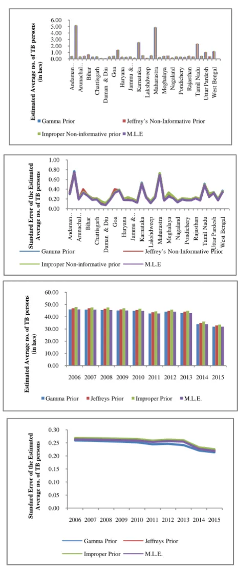
Table one reveals the average number of tuberculosis patients that has been calculated by using various prior distribution along with the standard error. The data for the average number of tuberculosis patient is national and state wise while the average number of tuberculosis patients year wise by using various prior distribution is discussed in the table two.

Fig. 1 0.00 1.00 2.00 3.00 4.00 5.00 6.00 A n da m an … A run ac h al … B ih ar C h at ti sga rh D am an & D iu G o a H ar y an a Ja m m u & … K ar n at aka L aks h dw ee p M ah ar as tr a M egh al a y a N aga la n d P o n di ch er y R aj as th an T am il N adu U tt ar P ar de sh W es t B en ga l E st im at ed A ve rage n o. of T B p er son s (i n l ac s)

Gamma Prior Jeffrey’s Non-Informative Prior Improper Non-informative prior M.L.E

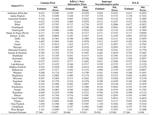
0.00 0.20 0.40 0.60 0.80 1.00 A n da m an … A run ac h al … B ih ar C h at ti sga rh D am an & D iu G o a H ar y an a Ja m m u & … K ar n at aka L aks h dw ee p M ah ar as tr a M egh al a y a N aga la n d P o n di ch er y R aj as th an T am il N adu U tt ar P ar de sh W es t B en ga l S tan d ar d E rr or of t h e E st im at ed A ve rage n o. of T B p er son s

Gamma Prior Jeffrey’s Non-Informative Prior Improper Non-informative prior M.L.E

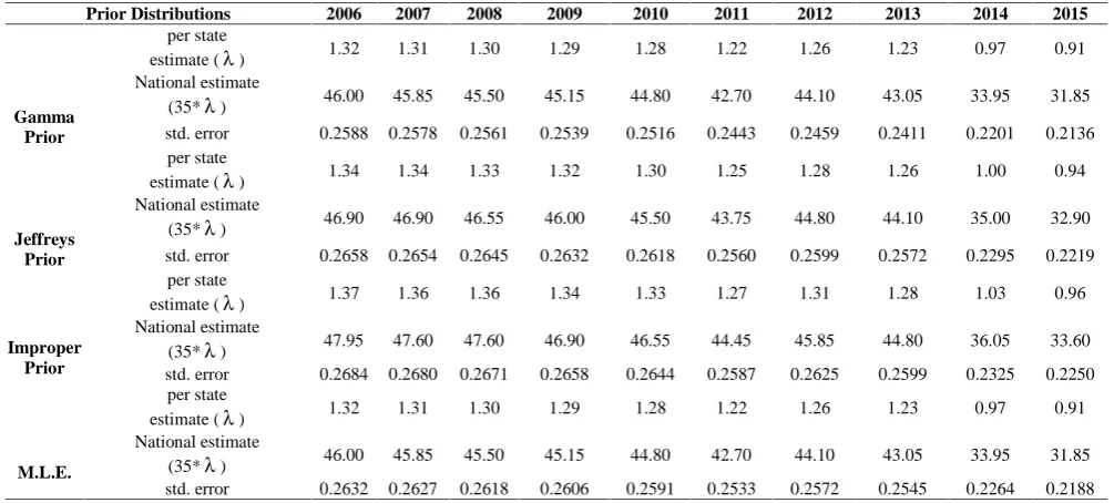
0.00 10.00 20.00 30.00 40.00 50.00 60.00

2006 2007 2008 2009 2010 2011 2012 2013 2014 2015

E st im at ed A ve rage n o. of T B p er son s (i n l ac s)

Gamma Prior Jeffreys Prior Improper Prior M.L.E.

0.00 0.05 0.10 0.15 0.20 0.25 0.30

2006 2007 2008 2009 2010 2011 2012 2013 2014 2015

S tan d ar d E rr or of t h e E st im at ed A ve rage n o. of T B p er son s

(5)

The spread of the average number of tuberculosis patients

among various states/UT’s across different years has been

obtained in table one and two. Along with the average number of tuberculosis patients their corresponding standard errors has been computed. Figure 1 an 3 reveals that for a Gamma prior Maximum likelihood estimation method is as similar as Empirical Bayes estimation. For this reason instead of being fully-Bayesian, Empirical Bayesian is sometimes labeled as non-Bayesian or as partially-Bayesian. The standard error that has been obtained from these different estimators are not identical which is also revealed in the figure two and four which becomes a criteria for not preferring or preferring Bayesian procedure of introducing in the estimation function the prior distribution.

In the table 1 when the average number of tuberculosis patient is estimated state-wise, time is treated as a random variable in that case and while making the analysis it has been found that the minimum standard errors given by the Maximum Likelihood estimates which is also revealed by the figure2. The estimator that has been produced by the Maximum Likelihood estimation are not much better than the estimators that has been obtained by the use of prior distribution in which the additional information has been routed. Rather, it shows that there is a gradual move from the informative priors to non-informative priors (as the Maximum Likelihood estimation involves no prior distribution it is the most non-informative one), and as the

estimates moves from informative one to non information one there is a reduction in value of their standard errors. The estimators that have been obtained for the incidence of tuberculosis is computed by assuming them as time independent constant, this may be one of the possible for the trend that has been obtained above and such estimators may not be viable when random variable is time. When the hyper parameters are time dependent it may become one of the possible solution to the situation.

When the random variable is States/UT’s and the time was kept

as fixed variable, the minimum standard error in that type of model is given by the Bayes estimates with Gamma prior which is subsequently followed by the estimates obtained by

the maximum Likelihood estimates and Jeffrey’s and improper

prior which is also revealed by the table 2. Thus in such sort of cases it is admissible and proved that the Bayes estimates are better than the conventional Maximum Likelihood estimates. The last points that have been made in previous paragraph could be the reason for the standard error of the estimates to be much better than Maximum Likelihood Estimation. These overwhelming better results are also shown in the figure 4. As one may thought of the difference that exist among the standard error obtained from different estimators appears to be meager but it is considered as a way significant enough to prefer one procedure over the other because the number that has been associated is in lakhs.

Table 1 Bayes estimates and Standard errors of the average TB persons (Lakhs) in variousStates/UT’s of India

States/UT’s

Gamma Prior Jeffrey’s Non -Informative Prior

Improper

Non-informative prior M.L.E

Estimate Std.

Error Estimate

Std.

(6)

CONCLUSIONS

The results that have been computed show the declining trend in the average number of tuberculosis infected patients in India over the years. The high incidence of the tuberculosis patients is recorded in the states of Maharashtra and Andhra Pradesh while the states of Nagaland and Jharkhand shows the lowest incidence of tuberculosis cases. The states that have high prevalence of tuberculosis and which also shows the increase in incidence in year 2015 as compared to 2006 are Karnataka, Andhra Pradesh, Tamil Nadu and Maharashtra. While considering the prevalence of number of tuberculosis patients per square kilometer, the highest incidence is recorded by Delhi while the lowest incidence is recorded by Rajasthan. Nagaland and Manipur have the highest percentage of tuberculosis cases in terms of population of each state while Jharkhand has the lowest percentage.

The results by not discrimination one from the other invariable strikes a sort of balance between the Bayesian procedure and the Classical Procedure. Bayesian procedure simply encompasses the classical procedure by making assumption regarding the hyper parameters. For calculating the national average of the tuberculosis patients, this procedure can be generalized. However there are scopes for making further improvement in the development of such a procedure which also takes into account the time dependent incidence rate. Such a model would then help in refining the Bayes estimator even for time series data to perform well. It has been verified that the incidence rate depends upon certain covariates and we can apply suitable Bayesian approach to it.

References

1. Alfred A. Bartolucci, Karan P. Singh, Ramalingham

Shanmugam, 2004, “Empirical Bayesian analysis of the Poisson intervention and incidence parameters,”

Mathematics and Computers in Simulation, Vol. 64, 393-399.

2. Alphonse Kpozèhouen, Ahmadou Alioum, et al., 2004,

“Use of a Bayesian Approach to Decide When to Stop a

Therapeutic Trial: The Case of a Chemoprophylaxis

Trial in Human Immunodeficiency Virus Infection,”

American Journal of Epidemiology, Volume 161, Issue

6, 595-603.

3. Berry, D.A., Wolff, M.C., Sack, D., 1994, “Decision making during a phase III randomized controlled trial,”

Controlled Clinical Trials, 15, 360-78.

4. Brenner, D., Fraser, D.A.S., and McDunnough, P., 1982,

“On asymptotic normality of likelihood and conditional

analysis,” can.J. Statist., 10, 163-172.

5. Deuchert E, Brody S., 2007, “Plausible and implausible

parameters for mathematical modeling of nominal

heterosexual HIV transmission,” Ann Epidemiol., 17(3),

237-44.

6. Fraser, D.A.S., and McDunnough, P. (1984). “Further

remarks on asymptotic normality of likelihood and

conditional analysis,” can.J. Statist., 12, 183-190.

7. Nel A, Louw C, Hellstrom E, Braunstein SL, Treadwell I, et al. (2011). “HIV Prevalence and Incidence among

Sexually Active Females in Two Districts of South

Africa to Determine Microbicide Trial Feasibility,”

PLoS ONE 6(8): e21528. doi:10.1371/ journal. pone.0021528.

8. Pandey A, Sahu D, Bakkali T, et al. (2012), “Estimate of

HIV prevalence and number of people living with HIV in India 2008-2009,” BMJ open 2012;2:e000926.

doi:10.1136/bmjopen-2012-000926.

9. Robbins, H., 1955, “An Empirical Bayes Approach to Statistics,” in 119-127. Proceedings of the 3rd Berke-ley Symposium on MathematicaI Statistics and Probability (Vol. l), Berkeley, CA: University of California Press, 157-163.

10. K.O. Bowman and L.R. Shenton, Properties of Estimators for the Gamma Distribution, Marcel Decker, NewYork, 1988.

Table 2 Bayes estimates and standard errors of the average TB persons (Lakhs)

in India for the years 2006-2015

Prior Distributions 2006 2007 2008 2009 2010 2011 2012 2013 2014 2015

Gamma Prior

per state

estimate () 1.32 1.31 1.30 1.29 1.28 1.22 1.26 1.23 0.97 0.91 National estimate

(35*) 46.00 45.85 45.50 45.15 44.80 42.70 44.10 43.05 33.95 31.85 std. error 0.2588 0.2578 0.2561 0.2539 0.2516 0.2443 0.2459 0.2411 0.2201 0.2136

Jeffreys Prior

per state

(35*) 46.90 46.90 46.55 46.00 45.50 43.75 44.80 44.10 35.00 32.90 std. error 0.2658 0.2654 0.2645 0.2632 0.2618 0.2560 0.2599 0.2572 0.2295 0.2219

Improper Prior

per state

(35*) 47.95 47.60 47.60 46.90 46.55 44.45 45.85 44.80 36.05 33.60 std. error 0.2684 0.2680 0.2671 0.2658 0.2644 0.2587 0.2625 0.2599 0.2325 0.2250

M.L.E.

per state

(7)

11. R.L. Johnson, S. Kotz, and N. Balakrishnan, Continuous Univariate Distribution, 2nd ed., Vol. 1, Wiley, NewYork, 1995.

12. E. Damsleth, Conjugate classes for gamma distribution, Scand. J. Stat. 2 (1975), pp. 80–84.

13. R.B. Miller, Bayesian analysis of the two-parameter gamma distribution, Technometrics 22 (1980), pp. 65–

69.

*******

How to cite this article: