DOI10.1186/2190-5983-1-3
R E S E A R C H Open Access
Certified reduced basis approximation for parametrized
partial differential equations and applications
Alfio Quarteroni·Gianluigi Rozza· Andrea Manzoni
Received: 2 March 2011 / Accepted: 3 June 2011 / Published online: 3 June 2011
© 2011 Quarteroni et al.; licensee Springer. This is an Open Access article distributed under the terms of the Creative Commons Attribution License
Abstract Reduction strategies, such as model order reduction (MOR) or reduced basis (RB) methods, in scientific computing may become crucial in applications of increasing complexity. In this paper we review the reduced basis methods (built upon a high-fidelity ‘truth’ finite element approximation) for a rapid and reliable approxi-mation of parametrized partial differential equations, and comment on their potential impact on applications of industrial interest. The essential ingredients of RB method-ology are: a Galerkin projection onto a low-dimensional space of basis functions properly selected, an affine parametric dependence enabling to perform a competitive Offline-Online splitting in the computational procedure, and a rigorousa posteriori error estimation used for both the basis selection and the certification of the solu-tion. The combination of these three factors yields substantial computational savings which are at the basis of an efficient model order reduction, ideally suited for real-time simulation and many-query contexts (for example, optimization, control or pa-rameter identification). After a brief excursus on the methodology, we focus on linear elliptic and parabolic problems, discussing some extensions to more general classes of problems and several perspectives of the ongoing research. We present some
re-A Quarteroni·G Rozza (
)·A ManzoniModelling and Scientific Computing, CMCS, Mathematics Institute of Computational Science and Engineering, MATHICSE, Ecole Polytechnique Fédérale de Lausanne, EPFL, Station 8, CH-1015 Lausanne, Switzerland
e-mail:[email protected]
A Quarteroni
e-mail:[email protected]
A Manzoni
e-mail:[email protected]
A Quarteroni
sults from applications dealing with heat and mass transfer, conduction-convection phenomena, and thermal treatments.
1 Introduction and motivation
Although the increasing computer power makes the numerical solution problems of very large dimensions that model complex phenomena essential, a computational re-duction is still determinant whenever interested inreal-time simulations and/or re-peatedoutputevaluations for different values of someinputsof interest. For a general introduction on the development of the reduced basis methods we refer to [1–3].
In this work we review the reduced basis (RB) approximation anda posteriori error estimation methods for the rapid and reliable evaluation of engineering out-puts associated with elliptic and parabolic parametrized partial differential equations (PDEs). In particular, we consider a (say, single) output of interest s(μ)∈R ex-pressed as a functional of a field variableu(μ)that is the solution of a partial differen-tial equation,parametrizedwith respect to the input parameterp-vectorμ; theinput parameterdomain - that is, the set of all possible inputs - is a subsetDofRp. The
input-parametervector typically characterizes physical properties and material, geo-metrical configuration, or even boundary conditions and force fields or sources. The outputs of interestare physical quantities or indexes used to measure and assess the behavior of a system, that is, related to fields variables or fluxes, as for example, do-main or boundary averages of the field variables, or other quantities such as energies, drag forces, flow rates, and so on. For the sake of simplicity, we consider through-out the paper the case of a linear through-output of a field variable, that is,s(μ)=l(u(μ))
for a suitable linear operatorl(·). Finally, thefield variablesu(μ)that link the input parameters to the output depend on the selected PDE models and may represent tem-perature or concentration, displacements, potential functions, distribution functions, velocity or pressure. We thus arrive at aninput-outputrelationshipμ→s(μ), whose evaluation requires the solution of a parametrized PDE.
the reduced basis approximates not the exact solution but rather a ‘given’ finite ele-ment discretization of (typically) very large dimensionN, indicated as a high-fidelity truthapproximation. In short, we promote an algorithmic collaboration rather than a computational competition between RB and FE methods.
In this paper we shall focus on the case of linear functional outputs of affinely parametrized linear elliptic and parabolic coercive partial differential equations. This kind of problems - relatively simple, yet relevant to many important applications in transport (for example, steady/unsteady conduction, convection-diffusion), mass transfer, and more generally in continuum mechanics - proves a convenient exposi-tory vehicle for the methodology, with the aim of stressing on the potential impact on possible industrial applications, dealing with optimization for devices and/or pro-cesses, diagnosis, control.
We provide here a short table of contents for the remainder of this review paper. For a wider framework on the position occupied by reduced basis method compared with other reduced order modelling (ROM) techniques and their current develop-ments and trends, see [1]. After a brief historicalexcursus, we present in Section2
the state of the art of the reduced basis method, presenting the essential components of this approach. We describe the affine linear elliptic and parabolic coercive settings in Section3, discussing briefly admissible classes of piecewise-affine geometry and coefficients. In Sections4and5we present the essential components of the reduced basis method: RB Galerkin projection and optimality; greedy sampling procedures; anOffline-Onlinecomputational stratagem. In Section6we recall rigorous and rel-atively sharpa posteriorierror bounds for RB approximations of field variables and outputs of interest. In Section7we briefly discuss several extensions of the method-ology to more general and difficult classes of problems and applications, while in Section8we introduce three ‘working examples’ which shall serve to illustrate the RB formulation and its potential. In the last Section9we provide some future per-spectives.
Although this paper focuses only on the affine linear elliptic and parabolic coer-cive cases - in order to allow to catch all the main ingredients - the reduced basis ap-proximation and associateda posteriorierror estimation methodology is much more general; nevertheless, many problems can successfully be faced in the even simplest affine case.
2 State of the art of the methodology
In this section we briefly review the current landscape starting from a brief historical excursus, introduce the essential RB ingredients and provide several references for further inquiry.
2.1 Computational opportunities and collaborations
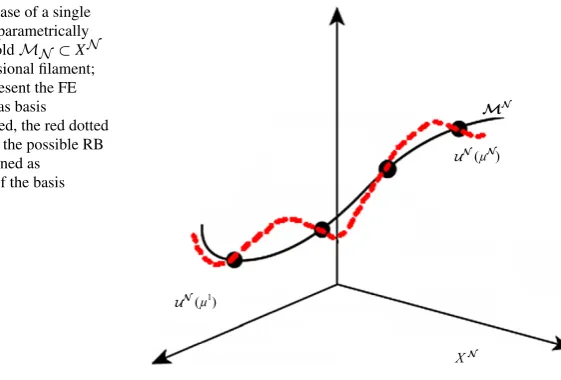
Fig. 1 In the case of a single parameter, the parametrically induced manifoldMN⊂XN
is a one-dimensional filament; the bullets represent the FE solutions used as basis functions. Indeed, the red dotted line denotes all the possible RB solutions, obtained as combinations of the basis functions.
many-query contexts represent also computational opportunities, since an important role in the RB paradigm and computational stratagem is played by the parametric setting. In particular:
(i)Our attention is restricted to a typically smoothand rather low-dimensional parametrically induced manifoldM, spanned by the set of fields engendered as the input varies over the parameter domain: for example, in the elliptic case
M=u(μ)∈X:μ∈D,
whereXis a suitable functional space. Clearly, generic approximation spaces are un-necessarily rich and hence unun-necessarily expensive within the parametric framework. Our approach is premised upon a classical finite element method ‘truth approxima-tion’ spaceXN ⊂Xof (typically very large) dimensionN; the RB method consists in a low-order approximation of the ‘truth’ manifoldMN (see Figure1) given by
MN =uN(μ)∈XN : μ∈D. (1)
Several classical RB proposals focus on the truth manifoldMN; much of what we present shall be relevant to any of these reduced basis spaces/approximations.
2.2 A brief historical path
Reduced Basis discretization is, in brief, a Galerkin projection on anN-dimensional approximation space that focuses on the parametrically induced manifoldMN. We restrict the attention to the Lagrange reduced basis spaces, which are based on the use of ‘snapshot’ FE solutions of the PDEs, corresponding to certain (properly selected) parameter values, as global approximation basis functions previously computed and stored; other possible approaches, such as Taylor [4] or Hermite spaces [5], take into account also partial derivatives of these basis solutions.
Initial ideas grew out of two related research topics dealing with linear/nonlinear structural analysis in the late 70’s: the need for more effective many-query design evaluation and more efficient parameter continuation methods [6–8]. The first work presented in these early somewhat domain-specific contexts were soon extended to (i) general finite-dimensional systems as well as certain classes of ODEs/PDEs [9–
12], and (ii) a variety of different reduced basis approximation spaces - in particular Taylor and Lagrange and more recently Hermite expansions. The next decade saw further expansion into different applications and classes of equations, such as fluid dynamics and, more specifically, the incompressible Navier-Stokes equations [13–
16].
However, in these early methods, the approximation spaces tended to be rather local and typically low-dimensional in parameter (often a single physical parameter), due also to the absence ofa posteriorierror estimators and effective sampling pro-cedures. It is clear that in higher-dimensional parameter domains thead hocreduced basis predictions ‘far’ from any sample points can not necessarily be trusted, and hencea posteriorierror estimators combined with efficient parametric space explo-ration techniques are crucial to guarantee reliability, accuracy and efficiency.
Much current effort in the last ten years in the RB framework has thus been de-voted to the development of (i)a posteriorierror estimation procedures - and in par-ticular rigorous error bounds for outputs of interest - and (ii) effective sampling strate-gies, in particular for higher dimensional parameter domains [17,18]. Thea posteri-orierror bounds are of course mandatory for rigorous certification of any particular RB Online output prediction. Not only, ana prioritheory for RB approximations is also available, dealing with a class of single parameter coercive problems [19] and more recently extended also to the multi-parameter case [20].
However, the error estimators also play an important role in effective (greedy) sampling procedures [1,18]: they allow us to explore efficiently the parameter do-main in search of most representative ‘snapshots’, and to determine when we have just enoughbasis functions. We note here that greedy sampling methods are similar in objective to, but very different in approach from, more well-known Proper Or-thogonal Decomposition (POD) methods [21]; the former are usually applied in the (multi-dimensional) parameter domain, while the latter are most often applied in the (one-dimensional) temporal domain. An efficient combination of the two techniques greedy-PODin parameter-time has been proposed [22,23] and is currently used for the treatment of parabolic problems [24]; see Section5.2.
approximation - with space of very high dimensionN - from the subsequent reduced basis projection and evaluation - of very low dimensionN. Consequently, the compu-tational savings provided by RB treatment (relative to classical FE evaluation) were typically rather modest [4,7,10]despitethe very small size of the RB linear sys-tems. Much work has thus been devoted tofulldecoupling of the FE and RB spaces through Offline-Online procedures, above all concerning the efficienta posteriori er-ror estimation: the complexity of the Offline stage depends onN; the complexity of the Online stage - solution and/or output evaluation for a new value ofμ- depends only onN andQ(used to measure the parametric complexity of the operator and data, as defined below). In this way, in the Online stage we can reach the accuracy of a high-fidelity FE model but at the very low cost of a reduced-order model.
In the context ofaffine parameter dependence, in which the operator is express-ible as the sum of Q products of dependent functions and parameter-independent operators (see Section3), the Offline-Online idea is quite self-apparent and has been naturally exploited [16, 25] and extended more recently in order to obtain efficienta posteriorierror estimation. In the case ofnonaffine parameter de-pendence the development of Offline-Online strategies is even more challenging and only in the last few years effective procedures have been studied and applied [26] to allow more complex parametrizations; clearly, Offline-Online procedures are an important element both in the real-time and the many-query contexts. We recall that also historically [9] RB methods have been built upon, and measured (as regards accuracy) relative to, underlyingfinite elementdiscretizations. However, spectral el-ement approaches [27,28], finite volume [22], and other traditional discretization methods may be considered too.
2.3 Essential RB components
The essential components of the reduced basis method, which will be analyzed in detail along the next sections, can be summarized as below.
(i) Rapidly convergent global reduced basis (RB) approximations - (Galerkin) pro-jection onto a (Lagrange) spaceXNN spanned by solution of the governing par-tial differenpar-tial equation atN (optimally) selected pointsSN in the parameter
setD. Typically,N will be small, as we focus attention on the (smooth) low-dimensional parametrically-induced manifold of interest. The RB approxima-tions to the field variable and output will be denoteduN(μ)andsN(μ),
respec-tively.
(ii) Rigorousa posteriorierror estimation procedures that provide inexpensive yet sharp bounds for the error in the RB field-variable approximation,uN(μ), and
output(s) approximation,sN(μ). Our error indicators are rigorous upper bounds
for the error (relative to the FE truth fielduN(μ)and outputsN(μ)=l(uN(μ))
approximation, respectively) for allμ∈Dand for allN. Error estimators are also employed during the greedy procedure [1] to construct optimal RB sam-ples/spaces ensuring an efficient and well-conditioned RB approximation. (iii) Offline/Online computational procedures - decomposition stratagems which
the way for subsequent inexpensive calculations performed Onlinefor each new input-output evaluation required.
3 Elliptic & parabolic parametric PDEs
We introduce the formulation of affinely parametrized linear elliptic/parabolic coer-cive problems; the methodology addressed in this work is intended for heat and mass convection/conduction problems. For the sake of simplicity, we consider only com-pliant outputs, referring to Section7 for the treatment of general (non-compliant) outputs and the extensions to other classes of equations.
3.1 Elliptic coercive parametric PDEs
We consider the following problem: Givenμ∈D⊂Rp, evaluate the output of inter-est
s(μ)=u(μ), (2)
whereu(μ)∈X()satisfies
au(μ), v;μ=f (v), ∀v∈X(). (3)
is a suitably regular bounded spatial domain inRd (for d=2 or 3), X=X()
is a suitable Hilbert space;a(·,·;μ)andf (·;μ)are the bilinear and linear forms, respectively, associated with the PDE. We shall exclusively consider second-order PDEs, and hence(H01())ν⊂X()⊂(H1())ν, whereν=1 (respectively,ν=d) for a scalar (respectively, vector) field; here L2() is the space of square inte-grable functions over,H1()= {v|v∈L2(),∇v∈(L2())d},H01()= {v∈ H1():v|∂=0}. We denote by(·,·)Xthe inner product associated with the Hilbert
spaceX, whose induced norm · X= √
(·,·)Xis equivalent to the usual(H1())ν
norm. Similarly,(·,·)and · denote theL2()inner product and induced norm, respectively.
We shall assume that thebilinearforma(·,·;μ):X×X→Riscontinuousand coerciveoverXfor allμinD, that is,
γ (μ):=sup
w∈X
sup
v∈X
a(w, v;μ) wXvX
<+∞, ∀μ∈D, (4)
∃α0>0:α(μ):= inf
w∈X
a(w, w;μ)
w2X ≥α0, ∀μ∈D. (5)
Finally,f (·)and(·)are linear continuous functionals overX; we assume - solely for simplicity of exposition - thatf andare independent ofμ. Under these standard hypotheses onaandf, (3) admits a unique solution. For the sake of simplicity,1we
1This assumption will greatly simplify the presentation while still exercising most of the important RB
shall further presume for most of this paper that we are in ‘compliance’ case [1]. In particular, we assume that (i)a is symmetric -a(w, v;μ)=a(v, w;μ),∀w, v∈X,
∀μ∈D- and furthermore (ii)=f. We shall make one last assumption, crucial to Offline-Online procedures, by assuming that the parametric bilinear formais ‘affine’ in the parameterμ: for some finiteQa,a(·,·;μ)can be expressed as
a(w, v;μ)= Q
q=1
qa(μ)aq(w, v), (6)
for given smooth μ-dependent functions qa, 1 ≤q ≤ Qa, and continuous μ
-independent bilinear formsaq, 1≤q≤Qa (in the compliant case theaq are
ad-ditionally symmetric). Under this assumption,MN defined by (1) lies on a smooth
p-dimensional manifold inXN. In actual practice,f may also depend affinely on the parameter: in this case,f (v;μ)may be expressed as a sum ofQf products of
μ-dependent functions andμ-independentX-bounded linear forms. As we shall see in the following, the assumption of affine parameter dependence isbroadly relevant to many instances of both propertyandgeometry parametric variation. Nevertheless, this assumption may be relaxed [26], as detailed in Section7.
3.2 Parabolic coercive parametric PDEs
We also consider the following parabolic model problem: Givenμ∈D⊂Rp, evalu-ate the output of interest
s(t;μ)=u(t;μ), ∀t∈I= [0, tf], (7)
whereu(μ)∈C0(I;L2())∩L2(I;X)is such that
m
∂u
∂t(t;μ), v;μ
+au(t;μ), v;μ=g(t )f (v), ∀v∈X,∀t∈I, (8)
subject to initial conditionu(0;μ)=u0∈L2();g(t )∈L2(I )is calledcontrol func-tion. In addition to the previous assumptions (4)-(6), we shall assume thata(·,·;μ) -which represents convection and diffusion - is time-invariant; moreover,m(·,·;μ) -which represents ‘mass’ or inertia - is assumed to be time-invariant, symmetric, and continuous and coercive overL2(), with coercivity constant
∃σ0: σ (μ):= inf
w∈X
m(w, w;μ)
w2X ≥σ0, ∀μ∈D. (9)
Finally, we assume that alsom(·,·;μ)is ‘affine in parameter’, that is, it can be ex-pressed as
m(w, v;μ)= Qm
q=1
qm(μ)mq
(w, v), (10)
for givensmoothparameter-dependent functionsqm, 1≤q≤Qm, and continuous
3.3 Parametrized formulation
We now describe a general class - through not the most general one - of elliptic and parabolic problems which honors the hypotheses previously introduced; for simplic-ity we consider a scalar field (ν=1) in two space dimension (d=2). We shall first define an ‘original’ problem (subscripto), posed over theparameter-dependent do-maino=o(μ); we denoteXo(μ)a suitable Hilbert space defined ono(μ). In
the elliptic case, the original problem reads as follows: Givenμ∈D, evaluate
so(μ)=lo
uo(μ)
,
whereuo(μ)∈Xo(μ)satisfies
ao
uo(μ), v;μ
=fo(v), ∀v∈Xo(μ).
In the same way, for the parabolic case we have: Givenμ∈D, evaluate
so(t;μ)=lo
uo(t;μ)
,
beinguo(μ)∈C0(I;L2())∩L2(I;Xo(μ))such that mo
∂uo
∂t (t;μ), v;μ
+ao
uo(t;μ), v;μ
=g(t )fo(v), ∀v∈Xo(μ),∀t∈I.
The RB framework requires a reference (μ-independent) domainin order to com-pare, and combine, FE solutions that would be otherwise computed on different domains and grids. For this reason, we need to map o(μ)to a reference domain =o(μref), μref∈D, in order to get the ‘transformed’ problem (2)-(3) or (7 )-(8) - which is the point of departure of RB approach - for elliptic and parabolic case, respectively. The reference domainis thus related to the original domaino(μ)
through a parametric mappingT (·;μ), such thato(μ)=T (;μ). It remains to
place some restrictions on both the geometry (that is, ono(μ)) and the operators
(that is,ao,mo,fo,lo) such that (upon mapping) the transformed problem satisfies
the hypotheses introduced above - in particular, the affinity assumption (6), (10). To this aim, a domain decomposition is useful [1].
We first consider the class of admissible geometries. In order to build a paramet-ric mapping related to geometparamet-rical properties, we introduce a conforming domain decomposition ofo(μ),
o(μ)= Ldom
l=1
lo(μ), (11)
consisting of mutually nonoverlapping open subdomains lo(μ), s.t. lo(μ)∩ lo(μ)= ∅, 1≤l < l≤Ldom. If related to geometrical properties used as input parameters (for example, lengths, thicknesses, diameters or angles) the definition of parametric mappings can be done in a quite intuitive fashion.2 In the following
2These regions can represent different material properties, but they can also be used for algorithmic
we will identifyl =lo(μref), 1≤l≤Ldom, and denote (11) the ‘RB triangula-tion’; it will play an important role in the generation of the affine representation (6), (10). Hence, original and reference subdomains must be linkedvia a mapping
T (·;μ):l→lo(μ), 1≤l≤Ldom, such that
lo(μ)=Tll;μ, 1≤l≤Ldom; (12) these maps must be individually bijective, collectively continuous, and such that
Tl(x,μ)=Tl(x;μ),∀x∈l∩l, for 1≤l < l≤Ldom.
Here we consider the affine case, where the transformation is given, for anyμ∈D
andx∈l, by
Til(x,μ)=Cil(μ)+ d
j=1
Glij(μ)xj, 1≤i≤d, (13)
for given translation vectors Cl: D → Rd and linear transformation matrices Gl : D→Rd×d. The linear transformation matrices can effect rotation, scaling and/or shear and have to be invertible. The associated Jacobians can be defined as
Jl(μ)= |det(Gl(μ))|, 1≤l≤L
dom.
We next introduce the class ofadmissible operators. We may consider the associ-ated bilinear forms
ao(w, v;μ)= Ldom
l=1
l o(μ)
∂w ∂xo1
∂w ∂xo2w
Ko,l(μ)
⎡ ⎢ ⎣ ∂v ∂xo1 ∂v ∂xo2 v ⎤ ⎥
⎦, (14)
whereKo,l:D→R3×3, 1≤l≤Ldom, are prescribed coefficients.3In the parabolic
case, we also may consider
mo(w, v;μ)= Ldom
l=1
l o(μ)
wMo,l(μ)v, (15)
whereMo,l:D→Rrepresents the identity operator. Similarly, we require thatfo(·)
andlo(·)are written as
fo(v)= Ldom
l=1
l o(μ)
Fo,l(μ)v, lo(v)= Ldom
l=1
l o(μ)
Lo,l(μ)v,
whereFo,l:D→RandLo,l:D→R, for 1≤l≤Ldom, are prescribed coefficients.
By identifyingu(μ)=uo(μ)◦T (·;μ)in the elliptic case (resp.u(t;μ)=uo(t;μ)◦
3Here, for 1≤l≤L
dom,Ko,l:D→R3×3is a given SPD matrix (which in turn ensures coercivity of the bilinear form): the upper 2×2 principal submatrix ofKo,lis the usual tensor conductivity/diffusivity; the
(3,3)element ofKo,lrepresents the identity operator (‘mass matrix’) and is equal toMo,l; and the(3,1),
T (·;μ)∀t >0 in the parabolic case), and tracing (14) back on the reference domain
by the mappingT (·;μ), it follows that the transformed bilinear forma(·,·;μ)can be expressed as
a(w, v;μ)= Ldom
l=1
l ∂w ∂x1 ∂w ∂x2w
Kl(μ)
⎡ ⎢ ⎣ ∂v ∂x1 ∂v ∂x2 v ⎤ ⎥
⎦, (16)
whereKl:D→R3×3, 1≤l≤Ldom, is a parametrized tensor given by Kl(μ)=Jl(μ)Gl(μ)Ko,l(μ)
Gl(μ)T
andGl:D→R3×3is given by
Gl(μ)=
(Gl(μ))−10
0 1
, 1≤l≤Ldom.
In the same way, the transformed bilinear formm(·,·;μ)can be expressed as
m(w, v;μ)= Ldom
l=1
l
wMl(μ)v, (17)
whereMl:D→R, 1≤l≤Ldom,Ml(μ)=Jl(μ)Mo,l(μ). The transformed linear
forms can be expressed similarly as
f (v)= Ldom
l=1
Fl(μ)v, l(v)= Ldom
l=1
Ll(μ)v,
where Fl: D→R and Ll: D→R are given by Fl(μ)=Jl(μ)Mo,l(μ), Ll = Jl(μ)Lo,l(μ), for 1≤l≤Ldom. Hence, the original problem has been reformulated on a reference configuration, resulting in a parametrized problem where the effect of geometry variations is traced back onto its parametrized transformation tensors. The affine formulation (6) (resp. (6) and (10)) can then be derived by simply expanding the expression (16) (and (17)) in terms of the subdomainsland the different entries ofKijl . This results, for example, in
a(w, v;μ)=K111(μ)
1
∂w ∂x1
∂v ∂x1+
K112(μ)
1
∂w ∂x1
∂v ∂x2+ · · ·
.
bilinear formsaandm; we may consider coefficient functionsK,Mwhich are poly-nomial in the spatial coordinate (or more generally approximated by the Empirical Interpolation Method [26]). Some generalizations will be addressed in Section7and can be pursued by modification of the method presented in Section4: in general, increased complexity in geometry and operator will result in more terms in affine expansions - larger - with a corresponding increase in the reduced basis (Online) computational costs.
4 The reduced basis method
We discuss in this section all the details related to the construction of the reduced basis approximation in both the elliptic and the parabolic case, for rapid and reliable prediction of engineering outputs associated with parametrized PDEs.
4.1 Elliptic case
We assume that we are given a FE approximation spaceXN of (typically very large) dimensionN. Hence, the FE discretization of problem (2)-(3) [29,30] is as follows: givenμ∈D, evaluate
sN(μ)=uN(μ), (18)
whereuN(μ)∈XN satisfies
auN(μ), v;μ=f (v), ∀v∈XN. (19)
We then introduce, given a positive integerNmax, an associated sequence of (what shall ultimately be reduced basis) approximation spaces: forN=1, . . . , Nmax,XNN
is aN-dimensional subspace ofXN; we further suppose that they are nested (or hi-erarchical), that is,X1N ⊂XN2 ⊂ · · · ⊂XNN
max ⊂X
N; this condition is fundamental
in ensuring (memory) efficiency of the resulting RB approximation. We recall from Section2that there are several classical RB proposals - Taylor, Lagrange, and Her-mite spaces - as well as many different approaches, such as POD spaces. Even if we focus on Lagrange RB spaces, much of what is presented in this paper - in particular, concerning the discrete formulation, Offline-Online procedures anda posteriorierror estimation - shall be relevant to any of these RB spaces/approximations, even if they are not of immediate application in industrial problems (where we want to preserve the Offline-Online procedure and hierarchical spaces).
In order to define a (hierarchical) sequence of Lagrange spacesXNN, 1≤N ≤ Nmax, we first introduce a ‘master set’ of properly selected parameter pointsμn∈D, 1≤n≤Nmax. We then define, for givenN∈ {1, . . . , Nmax}, the Lagrange parameter samples
SN=
μ1, . . . ,μN, (20) and associated Lagrange RB spaces
the uN(μn), 1≤n≤Nmax, are often referred to as ‘(retained) snapshots’ of the parametric manifoldMN and are obtained by solving the FE problem (19) forμn,
1≤n≤Nmax. It is clear that, if indeed the manifold is low-dimensional and smooth, then we would expect to well approximate any member of the manifold - any solution
uN(μ)for someμ inD- in terms of relatively few retained snapshots. However, we must ensure that we can choose a good combination of the available retained snapshots; represent the retained snapshots in a stable RB basis, efficiently obtain the associated RB basis coefficients; and finally choose the retained snapshots (that is, the sampleSNmax) in an optimal way. The sampling strategy used to build the setSN will be discussed in Section5.
4.1.1 Galerkin projection
For our particular class of equations, Galerkin projection is arguably the best ap-proach. Givenμ∈D, evaluate (recalling the compliance assumption)
sNN(μ)=fuNN(μ), (22)
whereuNN(μ)∈XNN ⊂XN (or more precisely,uN
XNN(μ)∈X N
N) satisfies
auNN(μ), v;μ=f (v), ∀v∈XNN. (23)
We immediately obtain the classical optimality result in the energy norm:4
uN(μ)−uNN(μ)μ≤ inf
w∈XNN
uN(μ)−wμ; (24)
in the energy norm, the Galerkin procedure automatically selects thebest combina-tion of snapshots; moreover, we have that
sN(μ)−sNN(μ)=uN(μ)−uNN(μ)2μ, (25) that is, the output converges as the ‘square’ of the energy error. Although this latter result depends critically on the compliance assumption, extensionviaadjoint approx-imations to the non-compliant case is possible; we discuss this further in Section7.
We now consider the discrete equations associated with the Galerkin approxi-mation (23). First of all, we apply the Gram-Schmidt process with respect to the
(·,·)Xinner product to snapshotsuN(μn), 1≤n≤Nmax, to obtain mutually(·,·)X
-orthonormal basis functionsζnN, 1≤n≤Nmax. Then, the RB solution can be ex-pressed as:
uNN(μ)= N
m=1
uNN m(μ)ζmN; (26)
4Under the coercivity and the symmetry assumptions, the bilinear forma(·,·;μ)defines a (energy) scalar
product given by((w, v))μ:=a(w, v;μ)∀w, v∈X; the inducedenergynorm is given by|||w|||μ=
by takingv=ζnN, 1≤n≤N, into (23) and using (26), we obtain the RB ‘stiffness’ equations
N
m=1
aζmN, ζnN;μuNN m(μ)=fζnN, (27)
for the RB coefficientsuNN m(μ), 1≤m, n≤N; we can subsequently evaluate the RB output as
sNN(μ)= N
m=1
uNN m(μ)fζmN. (28)
4.1.2 Offline-Online procedure
The system (27) is nominally of small size: a set ofNlinear algebraic equations inN
unknowns. However, the formation of the stiffness matrix, and indeed the load vector, involves entitiesζnN, 1≤n≤N, associated with ourN-dimensional FE approxima-tion space. Fortunately, we can appeal to affine parameter dependence to construct very efficient Offline-Online procedures. In particular, system (27) can be expressed, thanks to (6), as
N
m=1
Q
q=1
q(μ)aqζmN, ζnN
uNN m(μ)=fζnN,
for 1≤n≤N. The equivalent matrix form is
Q
a
q=1
qa(μ)AqN
uN(μ)=fN, (29)
where(uN(μ))m=uNN m(μ)and
AqNmn=aqζmN, ζnN, (fN)n=f
ζnN,
for 1≤m, n≤Nmax. Since each basis functionζnN belongs to the FE spaceXN, they can be written as
ζnN =
N
i=1
ζniNφi, 1≤n≤Nmax,
that is, as a linear combination of the FE basis functions{φi}Ni=1; therefore, the RB ‘stiffness’ matrix can be assembled once the corresponding the RB ‘stiffness’ matrix can be assembled. Then, by denoting
we have that
AqN=ZTAqNZ, fN=ZTFN,
being
Aq
N
ij=a q(φ
j, φi), (FN)i=f (φi)
the structures given by the FE discretization. In this way, computation entails an ex-pensiveμ-independent Offline stage performed only once and an Online stage for any chosen parameter valueμ∈D. During the former the FE structures{AqN}Qa
q=1 andFN, as well as the snapshots{uN(μn)}Nmax
n=1 and the corresponding orthonormal basis{ζnN}Nmax
n=1, are computed and stored. In the latter, for any givenμ, all the
a q(μ)
coefficients are evaluated, and theN×Nlinear system (29) is assembled and solved, in order to get the RB approximationuNN(μ). Then, the RB output approximation is obtained through the simple scalar product (37). Although being dense (rather than sparse as in the FE case), the system matrix is very small, with a size independent of the FE space dimensionN.
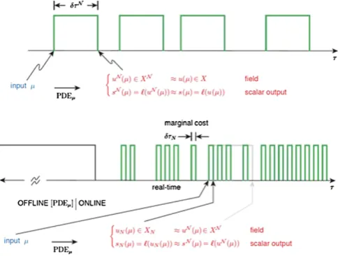
The Online operation count isO(QN2)to get andO(N3)to invert the matrix in (29), and finallyO(N )to effect the inner product (37). The Online storage is - thanks to the hierarchy assumption - onlyO(QNmax2 )+O(Nmax): for any given N, we may extract the necessary RBN×Nmatrices (respectively,N-vectors) as principal submatrices (respectively, principal subvectors) of the correspondingNmax×Nmax (respectively,Nmax) quantities. The Online (marginal) cost (operation count and stor-age) to evaluateμ→sNN(μ)is thus independent ofN (see Figure2).
Fig. 2 Comparison between the finite element and the reduced basis approximation frameworks:δτN
4.2 Parabolic case
We next introduce the finite difference in time and finite element (FE) in space dis-cretization [29,30] of the parabolic problem (8). We first divide the time intervalI
into K subintervals of equal length t =tf/K and definetk =kt, 0≤k≤K,
and define the FE approximation space XN. Hence, given μ∈D, we look for
uNk(μ)∈X, 0≤k≤K, such that
1
tm
uNk(μ)−uNk−1(μ), v;μ+auNk(μ), v;μ =g(tk)f (v), ∀v∈XN,1≤k≤K,
(30)
subject to initial condition(uN0, v)=(u0, v),∀v∈XN. We then evaluate the output (recalling the compliance assumption): for 0≤k≤K,
sNk(μ)=fuNk(μ). (31)
We shall sometimes denoteuNk(μ)asuN(tk;μ)andsNk(μ)assN(tk;μ)to more clearly identify the discrete time levels. Under the coercivity assumption (9) of the bilinear forma(·,·;μ)and the smoothness assumption ofqa,m(μ)coefficients,
MNK=uNk(μ):1≤k≤K,μ∈D, (32)
the analogous entity of (32) in the parabolic case, lies on a smooth (p+1) -dimensional manifold inXN.
Equation (30) - Backward Euler-Galerkin discretization of (8) - shall be our point of departure: we shall presume thattis sufficiently small andN is sufficiently large such that uN(tk;μ)andsN(tk;μ)are effectively indistinguishable from u(tk;μ)
ands(tk;μ), respectively. The development readily extends to Crank-Nicholson or higher order discretization; for purposes of exposition, we consider the simple Back-ward Euler approach.
The RB approximation in this case [24,31] is based on RB spacesXNN, 1≤N≤ Nmax, generated by a sampling procedure which combines spatial snapshots in time and parameter -uNk(μ)- in an optimal fashion (see Section5). Givenμ∈D, we now look forukN(μ)∈XNN, 0≤k≤K, such that
1
tm
ukN(μ)−ukN−1(μ), v;μ+aukN(μ), v;μ =gtkf (v), ∀v∈XNN,1≤k≤K,
(33)
subject to(u0N(μ), v)=(uN0, v),∀v∈XNN. We then evaluate the associated output: for 0≤k≤K,
sNk(μ)=fukN(μ). (34)
We shall sometimes denoteukN(μ) as uN(tk;μ)and skN(μ)as sN(tk;μ) to more
aN -XNN,uNNk(μ),sNNk(μ)- since the RB approximation is defined in terms of the truth discretization; however, for clarity of exposition, we shall typically suppress this superscript.)
We now develop the algebraic equations associated with (33)-(34). First of all, the RB approximationukN(μ)∈XNN shall be expressed as
ukN(μ)= N
m=1
ukN m(μ)ζmN, (35)
given a set of mutually(·,·)X orthogonal basis functionsζnN ∈XN, 1≤n≤Nmax,
and corresponding (hierarchical) RB spaces
XN=span{ξn,1≤n≤N}, 1≤N≤Nmax. By takingv=ζnN, 1≤n≤N, into (33) and using (35), we obtain:
1
t N
m=1
mζmN, ζnN;μukN m(μ)+ N
m=1
aζmN, ζnN;μukN m(μ)
=fζnN+ 1 t
N
m=1
mζmN, ζnN;μukN m−1(μ),
(36)
for the RB coefficientsuNN m(μ), 1≤m, n≤N; we can subsequently evaluate the RB output as
sNk(μ)= N
m=1
ukN m(μ)fζmN. (37)
The equivalent matrix form is
Q
a
q=1
qa(μ)A q N+ 1 t Qm
q=1
qm(μ)M q N
uN(μ)=fN+
1
t Qm
q=1
qm(μ)M q
N, (38)
where(ukN(μ))m=ukN m(μ)and
MqNmn=mqζmN, ζnN, 1≤m, n≤Nmax;
other terms are the same as in the elliptic case (see Sections4.1.1-4.1.2). Moreover, also the RB mass terms can be computed from the FE mass terms as
MqN=ZTMqNZ, where MqNij=mq(φj, φi),
being{φi}Ni=1the basis of the FE spaceXN.
as regards storage, we must now append to the elliptic Offline dataset an affine de-velopment for the mass matrixMqN, 1≤q≤Qm, associated with the unsteady term;
as regards computational complexity, we must multiply the elliptic operation counts byKto arrive atO(KN3)(in fact,O(KN2)for a linear time-invariant system) for the Online operation count, whereKis the number of time steps (recall that in actual practice the ‘truth’ is discrete in time). Thus, the Online evaluation ofsN(μ)remains
independent ofN even in the unsteady case.
5 Sampling strategies
We now review two sampling strategies used for the construction of RB spaces: a greedy procedure for the elliptic case and a combined POD-greedy procedure for the parabolic case. Let us denote bya finite sample of points inD, which shall serve as surrogates forDin the calculation of errors (and error bounds) over the parameter domain.
5.1 Elliptic case
We denote the particular samples which shall serve to select the RB space - or ‘train’ the RB approximation - bytrain. The cardinality oftrain will be denoted
|train| =ntrain. We note that although the ‘test’ samplesserve primarily to under-stand and assess the quality of the RB approximation anda posteriorierror estima-tors, the ‘train’ samplestrainserve togeneratethe RB approximation. The choice of ntrain andtrain thus have important Offline and Online computational implica-tions. Moreover, let us denoteε∗tola chosen tolerance for the stopping criterium of the greedy algorithm.
The greedy sampling strategy can be implemented as follows:
S1= {μ1}; computeuN(μ1);
X1=span{uN(μ1)};
forN=2:Nmax
μN=arg max
μ∈trainN−1(μ);
εN−1=N−1(μN);
ifεN−1≤εtol∗
Nmax=N−1;
end;
computeuN(μN);
SN=SN−1∪ {μN};
XN=XNN−1∪span{uN(μN)}; end.
As we shall describe in detail in Section6,N(μ)is a sharp, (asymptotically)
inex-pensive a posteriorierrorboundforuN(μ)−uN
Roughly, at iterationN the greedy algorithm appends to theretained snapshots that particular candidate snapshot - over all candidate snapshotsuN(μ),μ∈train -which is (predicted5by thea posteriorierror bound to be the) least well approximated by (the RB prediction associated to)XNN−1. We refer to [32] for a general analysis of the greedy algorithm and related convergence rates.
5.2 Parabolic case
The temporal evolution case is quite different: the greedy approach [31] can en-counter difficulties best treated by incorporating elements of the POD selection pro-cess [22]. Our sampling method thus combine the POD intk- to capture the causality associated with the evolution equation - with the greedy procedure inμ[1,18,31] - to treat efficiently the higher dimensions and more extensive ranges of parameter variation.
To begin, we summarize the basic POD optimality property: givenJ elements
wj ∈XN, 1≤j ≤J, POD({w1, . . . , wJ}, M) returnsM < J (·,·)X-orthonormal
functions{χm,1≤m≤M}such that the spacePM=span{χm,1≤m≤M}is
opti-mal, that is,
PM= arg inf YM⊂span{wj,1≤j≤J}
1
J J
j=1 inf
v∈YM
wj−v2X 1/2
,
whereYM denotes anM-dimensional linear space.
To initiate the POD-greedy sampling procedure we must specifytrain, an initial sampleS∗= {μ∗0}and a toleranceεtol∗ . The algorithm depends on two suitable inte-gersM1andM2 (the criterium behind their setting is addressed later) and reads as follows:
SetZ= ∅, S∗= {μ∗0},μ∗=μ∗0; WhileN≤Nmax,0
{χm,1≤m≤M1} =POD({uN(tk,μ∗),1≤k≤K}, M1);
Z← {Z,{χm,1≤m≤M1}};
N←N+M2;
{ξn,1≤n≤N} =POD(Z, N ); XN=span{ξn,1≤n≤N};
μ∗=arg maxμ∈trainN(t
K=t f;μ)
S∗← {S∗, μ∗};
end.
SetXN=span{ξn,1≤n≤N},1≤N≤Nmax.
As we shall describe in detail in Section 6, N(tk;μ) provides a sharp
inexpen-sive a posteriorierrorboundforuN(tk;μ)−uNN(tk;μ)X. In practice, we exit the
5Clearly the accuracy and cost of thea posteriorierror estimator
POD-greedy sampling procedure atN=Nmax≤Nmax,0for which a prescribed error tolerance is satisfied: to wit, we define
εN ,∗ max= max
μ∈train
N(tK;μ),
and terminate whenεN ,∗ max≤ε∗tol. Note, by virtue of the final re–definition, the POD-greedy generateshierarchicalspacesXN, 1≤N≤Nmax, which is computationally
very advantageous.
We chooseM1to satisfy an internal POD error criterion based on the usual sum of eigenvalues andεtol∗ ; we chooseM2≤M1to minimize duplication in the RB space. It is important to note that the POD-greedy method readily accommodates a repeat
μ∗in successive greedy cycles - new information will always be available and old in-formation rejected; in contrast, a pure greedy approach in bothtandμ[31], though often generating good spaces, can ‘stall’. Furthermore, since the POD is conducted in only one (time) dimension - with the greedy addressing the remaining (parameter) dimensions - the procedure remains computationally feasible even for large parame-ter domains and very extensive parameparame-ter train samples (and in particular in higher parameter dimensions).
Concerning the computational aspects, the crucial point is that the operation count for the POD-greedy algorithm is additive and not multiplicative inntrainandN; in contrast, in a pure POD approach, we would need to evaluate the FE ‘truth’ solution at thentraincandidate parameter values. As a result, in the POD-greedy approach we can takentrainrelatively large: we can thus anticipate RB spaces and approximations that provide rapid convergenceuniformlyover the parameter domain.
6 A posteriorierror estimation
Effectivea posteriorierror bounds for field variables and outputs of interest are cru-cial for both the efficiency and the reliability of RB approximations. As regards effi-ciency,a posteriorierror estimation permits us to (inexpensively) control the error, as well as to minimize the computational effort by controlling the dimension of the RB space. Not only, in the greedy algorithm the application of error bounds (as sur-rogates for the actual error) allows significantly larger training samplestrain⊂D and a better parameter space exploration at greatly reduced Offline computational cost. Concerningreliability,a posteriorierror bounds allows a confident exploita-tion of the rapid predictive power of the RB approximaexploita-tion. By means of an efficient a posteriorierror bound, we can make up for an error quantification for each new parameter valueμin the online stage and thus can make sure that feasibility (and safety/failure) conditions are verified.
safety margins). And third, the bounds must be veryefficient: the Online operation count and storage to compute the RB error bounds - the marginal average cost - must be independent ofN (and commensurate with the cost associated with the RB output prediction).
6.1 Elliptic case
Let us now considera posteriorierror bounds for the field variableuNN(μ)and the outputsNN(μ)in the elliptic case (22)-(23). We introduce two basic ingredients of our error bounds: the error residual relationship and coercivity lower bounds.
6.1.1 Basic ingredients
The central equation ina posterioritheory is the error residual relationship. In partic-ular, it follows from the problem statements foruN(μ), (19), anduNN(μ), (23), that the errore(μ):=uN(μ)−uNN(μ)∈XN satisfies
ae(μ), v;μ=r(v;μ), ∀v∈XN. (39)
Herer(v;μ)∈(XN)(the dual space toXN) is the residual,
r(v;μ):=f (v;μ)−auNN(μ), v;μ, ∀v∈XN. (40)
Indeed, (39) directly follows from the definition (40), f (v;μ)=a(uN(μ), v;μ),
∀v∈XN, bilinearity ofa, and the definition ofe(μ). It shall prove convenient to introduce the Riesz representation ofr(v;μ):e(μ)ˆ ∈XN satisfies
ˆ e(μ), v
X=r(v;μ), ∀v∈XN. (41)
This allows us to write the error residual equation (39) as
ae(μ), v;μ=e(μ), vˆ X, ∀v∈XN, (42)
and it follows that the dual norm of the residual can be evaluated through the Riesz representation:
r(·;μ)
(XN):= sup v∈XN
r(v;μ) vX
=e(μ)ˆ
X; (43)
this shall prove to be important for the Offline-Online stratagem developed in Sec-tion6.1.3below.
As a second ingredient, we need a positive, parametric lower bound function
αLBN(μ)forαN(μ), the FE coercivity constant6defined as
αN(μ)= inf
w∈XN
a(w, w;μ)
w2X ; (44)
6As we assumed that the bilinear form is coercive and the FE approximation spaces are conforming, it
hence, we introduce
0< αLBN(μ)≤αN(μ) ∀μ∈D, (45) where the online computational time to evaluateμ→αNLB(μ)has to be independent ofN in order to fulfill the efficiency requirements on the error bounds articulated be-fore. An efficient algorithm for the computation ofαLBN(μ)is given by the so-called Successive Constraint Method (SCM), widely analyzed in [1,33,34]. Moreover, the SCM algorithm - which is based on the successive solution of suitable linear op-timization problems - has been developed for the special requirements of the RB method; it thus features an efficient Offline-Online strategy, making the Online cal-culation complexity independent ofN - a fundamental requisite.
6.1.2 Error bounds
We define error estimators for the solution in the energy norm and for the output as
N(μ):=e(μ)ˆ X/
αLBN(μ)1/2, (46) and
sN(μ):=e(μ)ˆ X2 ≡2N(μ)/αLBN(μ), (47) respectively. We next introduce the effectivities associated with these error estimators as
ηN(μ):=N(μ)/uN(μ)−uNN(μ)μ,
and
ηNs (μ):=sN(μ)/sN(μ)−sNN(μ),
respectively. Clearly, the effectivities are a measure of the quality of the proposed es-timator: for rigor, we shall insist upon effectivities≥1; for sharpness, we desire effec-tivities as close to unity as possible. We can prove7[1] that for anyN=1, . . . , Nmax, the effectivities satisfy
1≤ηN(μ)≤
γ (μ)
αLBN(μ), ∀μ∈D, (48)
1≤ηNs (μ)≤ γ (μ)
αNLB(μ), ∀μ∈D, (49) γ (μ)being defined in (4). It is important to observe that the effectivity upper bounds, (48) and (49), areindependentofN, and hence stable with respect toRB refinement.
6.1.3 Offline-Online forˆe(μ)Xcomputation
The error bounds of the previous section are of no utility without an accompanying Offline-Online computational approach.
The computationally crucial component of all the error bounds of the previous section isˆe(μ)X, the dual norm of the residual. To develop an Offline-Online
pro-cedure we first expand the residual (40) according to (26) and (6):
r(v;μ)=f (v)−a
N
n=1
uNN n(μ)ζnN, v;μ
=f (v)− N
n=1
uNN n(μ)aζnN, v;μ
=f (v)− N
n=1
uNN n(μ) Q
q=1
q(μ)aqζnN, v.
(50)
If we insert (50) in (41) and apply linear superposition, we obtain
ˆ e(μ), v
X=f (v)− Q
q=1
N
n=1
q(μ)uNN n(μ)aqζnN, v,
or
ˆ
e(μ)=C+ Q
q=1
N
n=1
q(μ)uNN n(μ)Lqn,
where(C, v)X=f (v), ∀v∈XN, that is, C is the Riesz representation of f, and (Lqn, v)X= −aq(ζnN, v),∀v∈XN, 1≤n≤N, 1≤q≤Q, that is,L
q
nis the Riesz
representation ofAqn∈(XN)defined asAqn(v)=aq(ζnN, v),∀v∈XN. We denote
the C,Lqn, 1≤n≤N, 1≤q ≤Q, as FE ‘pseudo’-solutions, that is, solutions of
‘associated’ FE Poisson problems. We thus obtain
e(μ)ˆ 2X=(C,C)X+ Q
q=1
N
n=1
q(μ)uNN n(μ)
×
2C,Lqn
X+
Q
q=1
N
n=1
q(μ)uNN n(μ)Lqn,Lq n X , (51)
from which we can directly calculate the requisite dual norm of the residual through (43).
The Offline-Online decomposition is now clear. In the Offline stage we form the
μ-independent quantities. In particular, we compute the FE ‘pseudo’-solutions C,
Lq
n, 1≤n≤Nmax, 1≤q≤Q, and store(C,C)X,(C,Lqn)X,(Lqn,L q
n)X, 1≤n, n≤ Nmax, 1≤q, q≤Q. The Offline operation count depends onNmax,Q,andN.
In the Online stage, given any ‘new’ value ofμ- andq(μ), 1≤q≤Q,uNN n(μ), 1≤n≤N - we simply retrieve the stored quantities(C,C)X,(C,Lqn)X,(Lqn,Lq
1≤n, n≤N, 1≤q, q≤Q, and then evaluate the sum (51). The Online operation count, and hence also the marginal cost, isO(Q2N2)- andindependent of N.8 6.2 Parabolic case
In this section we deal witha posteriorierror estimation in the reduced basis context for affinely parametrized parabolic coercive PDEs. As for the elliptic case, to con-struct thea posteriorierror bounds we need two ingredients. The first ingredient is the dual norm of the residual
εN(tk;μ)= sup v∈XN
rN(v;tk;μ) vX
, 1≤k≤K, (52)
whererN(v;tk;μ)is the residual associated with the RB approximation (33)
rN
v;tk;μ=gtkf (v)− 1 tm
ukN(μ)−ukN−1(μ), v;μ −aukN(μ), v;μ, ∀v∈XN,1≤k≤K.
(53)
The second ingredient is a lower bound for the coercivity constant αN(μ), 0< αLBN(μ)≤αN(μ),∀μ∈D.
We can now define our error bounds in terms of these two ingredients; in fact, it can readily be proven [22,31] that for allμ∈Dand allN,
uNk(μ)−ukN(μ)μ≤kN(μ), (54)
sNk(μ)−sNk(μ)≤skN(μ), 1≤k≤K, (55)
wherekN(μ)≡N(tk;μ)andskN(μ)≡sN(tk;μ)are given by
kN(μ)=
t
αLBN(μ) k
k=1
εN2(tk;μ) 1/2
, (56)
skN(μ)=kN(μ)2. (57) (We assume for simplicity thatuN0∈XN; otherwise there will be an additional
con-tribution tokN(μ).)
Even if based on the same components as in the elliptic case, now the Construction-Evaluation procedure for the error bound is a bit more involved. The necessary com-putations for the Offline and Online stages - by construction rather similar to the elliptic case - are discussed in details, for example, in [24]. We consider here only the decomposition for the dual norm of the residual [31]. We first invoke duality, our RB
8It thus follows that thea posteriorierror estimation contribution to the cost of the greedy algorithm of
expansion, the affine parametric dependence ofaandm, and linear superposition to express
εN2tk;μ=QffN + N
n=1
Q
a
q=1
qa(μ)ukN n(μ)Q f a N nq+
1
t Qm
q=1
qm(μ)φN nk (μ)Q f m N nq
+ N ,N
n,n=1
Q
a,Qa
q,q=1
qa(μ)q
a(μ)ukN n(μ)ukN n(μ)Q aa N nnqq
+ 1 (t )2
Qm,Qm
q,q=1
qm(μ) q
m(μ)φN nk (μ)φN nk (μ)Q mm N nnqq
+ 1 t
Qa,Qm
q,q=1
qa(μ) q
m(μ)ukN n(μ)φ k N n(μ)Q
am N nnqq
,
(58)
for 1≤k≤K, whereφN nk (μ):=ukN n(μ)−uN nk−1(μ)andQffN =(zf, zf)X,Qf aN nq=
2(znqa , zf)X, 1≤q≤Qa, 1≤n≤N,QN nqf m =2(zmnq, zf)X, 1≤q≤Qm, 1≤n≤N, Qaa
N nnqq=(zanq, zanq)X, 1≤q, q≤Qa, 1≤n, n≤N,QamN nnqq=2(zanq, zmnq)X,
1≤ q ≤Qa, 1≤q ≤Qm, 1≤n, n ≤N, and QmmN nnqq =(z m
nq, zmnq)X, 1 ≤ q, q≤Qm, 1≤n, n≤N. Here thezf,zanq,zmnq are solutions to time-independent
and μ-independent ‘Poisson’ problems: (zf, v)X=f (v), ∀v ∈XN, (zanq, v)X= −aq(ξn, v), ∀v ∈ XN, 1 ≤n≤N, 1≤q ≤Qa, and (zmnq, v)X= −mq
(ξn, v), ∀v∈XN, 1≤n≤N, 1≤q≤Qm.
The Construction-Evaluation decomposition is now clear. In theμ-independent construction stage we findzf,za,zm, and the inner productsQffN
max,Q
f a Nmax,Q
f m Nmax,
Qaa Nmax,Q
mm
Nmax, andQ
am
Nmax at (considerable) computational costO(Q
·
aQ·mNmax· N·). In theμ-dependent Evaluation stage - performed many times - we simply perform the sum (58) from the stored inner products inO((1+QmN+QaN )2)operations
per time step and henceO((1+QmN+QaN )2K)operations in total. The crucial
point, again, is that the cost and storage in the Evaluation phase - themarginalcost for each new value ofμ- is independent ofN: thus we can not only evaluate our output prediction but also our rigorous output error bound very rapidly in the parametrically interesting contexts of real-time or many-query investigation.
7 Extensions to more general problems
7.1 Non-compliant problems
For the sake of simplicity, we addressed in Section4the RB approximation of affinely parametrized coercive problems in the compliant case. We now consider the elliptic case and the more general non-compliant problem: givenμ∈D, find
s(μ)=u(μ), (59)
whereu(μ)∈Xsatisfies
au(μ), v;μ=f (v), ∀v∈X. (60)
We assume that a is coercive and continuous (and affine, (6)) but not necessarily symmetric. We further assume that bothandf are bounded functionals but we no longer require=f.9 Following the methodology (and the notation) addressed in Section4, we can readily develop ana posteriorierror bound forsN(μ): by standard
arguments [1,2]
sN(μ)−sNN(μ)≤ (XN)N(μ),
where|||uN(μ)−uNN(μ)|||μ≤N(μ)andN(μ)is given by (46). We denote the
method already illustrated as ‘primal-only’. Although for many outputs primal-only is perhaps the best approach (each additional output, and associated error bound, is a simple ‘add-on’), this approach has two deficiencies:
(i) we loose the ‘quadratic convergence’ effect (25) for outputs (unless=f anda
is symmetric);
(ii) the effectivitiessN(μ)/|s(μ)−sN(μ)| may be unbounded: if=f then we
know, from (25), that |s(μ)−sN(μ)| ∼ ˆe(μ)2X and hence s(μ)/|s(μ)− sN(μ)| ∼1/ˆe(μ)X→ ∞asN→ ∞, that is, the effectivity of the output error
bound (47)tends to infinityas (N→ ∞and)uNNpr(μ)→uN(μ). We may expect
similar behavior for any‘close’ tof: the failing is that (47) does not reflect the contribution of the test space to the convergence of the output.
The introduction of RB primal-dualapproximation will take care of the previ-ous issue - and ensure a stable limitN→ ∞. We thus introduce the dual problem associated to, that reads as follows: findψ (μ)∈Xsuch that
a(v, ψ (μ);μ)= −(v), ∀v∈X;
ψis denoted the ‘adjoint’ or ‘dual’ field. Let us define the RB spaces for the primal and the dual problem, respectively:
XNN,pr pr =span
uNμk,pr≡ζkN,1≤k≤Npr
,
9Typical output fuctionals correspond to the ‘integral’ of the fieldu(μ)over an area or line (in particular,