A 2-D Barakat-Clark finite difference numerical method and its comparison for water quality simulation modeling

R E S E A R C H

Open Access

A 2-D Barakat-Clark finite difference numerical

method and its comparison for water quality

simulation modeling

Lei Jin

1*

, Aili Yang

1

, Li Wang

2

and Haiyan Fu

1

Abstract

Background:This paper provides an advance numerical algorithm to solve both ordinary and partial differential equations of surface water quality models. It uses finite difference methods and structures explicit or implicit or other process forms to solve the water quality model. This study also considers the stability of solutions to obtain more accurate results among those numerical algorithms.

Results:Water quality modeling commonly manifests itself in ordinary and partial differential equations in a realistic world. This study has applied numerical solutions to simulate the changing process of water quality in one and two dimensional spaces or in multiple dimensional spaces. The solutions of these analytical methods are provided in this paper to attest the justifiability of these numerical methods. It demonstrates that the 2-dimensional

Barakat-Clark numerical method can be a highly efficient tool in obtaining approximate results of ordinary and partial differential equations, which may prove difficult in finding the accurate solution by using conventional methods. At the same time, the stability analysis corroborated the convergence of those numerical solutions. Conclusions:This study is the first attempt to compare the multiple numerical methods with the 2-D Barakat-Clark method in the water quality modeling process. The results clearly suggest that the Barakat-Clark method is better in reflecting the accuracy of the water quality modeling with stability for hydrological systems.

Keywords:Water quality modeling; Numerical algorithm; 2-D barakat-clark method; Stability; Finite difference

Background

In the past few decades, the applications of surface water quality models have been intensely studied as population growth and economic development makes more increases pollution in water resources, particularly in the surface hydrological system. Streeter and Phelps have been pro-gressed the water quality models in 1925. Since then, many scientists (Kellogg 1964; Shampine et al. 1979; Stasa 1985; Christie 1987; Hoffman 1992; Rudi et al. 1997; Cash 2003; Shawgfeh 2004; Walter 2006) have carried out rigorous re-search in this area. Many water quality models, for example, the BOD model, are formed generally by ordinary or partial differential equations (Davis 1962; Na 1979; Taylor 1982; Evans 1985; Noye Noye 1992; Richard 1997; Moiianty 2004; Liu et al. 2005; Munavalli 2004; Timo et al. 2013). For

solving those equations, the traditional methods are using the finite difference method and the finite element method.

In this paper, the application of an explicit and an impli-cit method to solve the water quality equation includes and tests the first order ordinary differential equation, the second order ordinary differential equation and the sec-ond order partial differential equation. To illustrate the reasonability of these solutions, the stability of diffusion equations are also provided in this article. The analytic solutions obtained from these diffusion equations are also compared with other numerical methods. The results suggest that the numerical method can be as good to reflect the accurate solution of water quality diffusion equation in the real world condition.

Methods

Fundamental background of water quality modelling The transference, diffusion, and degradation mathematical equations of pollutants in the hydrological systems are * Correspondence:[email protected]

1

College of Environmental Science and Engineering, Xiamen University of Technology, Xiamen, Fujian Province 361024, China

Full list of author information is available at the end of the article

three-dimensional in form. Therefore, according to the mass balance equation, the initial water quality transfer equation is as follows:

∂C

∂t þ

X

i

Vi∂

C

∂Xi ¼

X

i ∂ ∂Xi εT;i

∂C

∂Xi

X

k

Sk

ð1aÞ

where

Xi= the three axial X1, X2, X3;

Vi= the velocity of three axial V1, V2, V3;

Sk= the source and sink of contaminants;

C = the concentrate of contaminants; t= time;

The C, ViandεT,iare the function of Xi. In the left side

of the equation (1a), the first item indicates the change rate of concentration of contaminants. The second item on the left side shows the transfer rate of contaminants along the stream axial. The first item, in the right hand side of the equation, presents the dispersion of pollutants along a different axial. There, we are assuming that there is no molecular diffusion and turbulent diffusion of pollut-ants. The second item in left side indicates the sources of contaminants. The symbol +/− states the contaminants increase or decrease in the hydrological systems. In (1a) is a three-dimensional variable coefficient of the second-order Partial Differential Equation (PDE). The parameters of mod-eling require much information; especially the variable S on the right side of equation, will cause a serious complication in the solution process. It is difficult to get the analytic a so-lution. Therefore, people usually simplified this modeling process then used the numerical method to generate the approximate solutions. This paper targets several simplified water quality models and uses finite difference method and structures simulate process forms to solve the problem. It also considers the stability of the solutions to obtain more accurate results among those numerical algorithms.

Numerical methods for water quality modeling Application of least squares method

If the velocity of the stream is very high, the variable of dispersion will be extremely low, so it can be ignored. Thus, the water shift modeling is presented as follows:

VdC

dX¼kC ð2aÞ

The equation (2a) is a first order ordinary differential equation. The analytic solution of it can be obtained as follow:

C¼C0e

k

Vx ð_3aÞ

Some of the parameters in (3a) can be solved by multiple linear regression method. Concurrently it can use the least

squares method to establish the error function. To consider the amount of biochemical oxygen demand (BOD) and disintegration, we useLto indicate BOD, andK1present disintegration coefficient of BOD. Then, equation (2a) can is presented as:

−dL

dt ¼K1L ð4aÞ

The solution of the above equation is L tð Þ ¼L0e−K1t.

Therefore the oxygen consumption isy tð Þ ¼L0−L tð Þ ¼L0

1−e−k1t

: By using experimental data, applying the least squares method estimates the initial value of L0and K1.

There letK1=K′1+hthen,

y tð Þ ¼L0 1−e−ðK′1þhÞt

h i

¼L0 1−e−K′1te−ht

ð5aÞ

lety(t) =af1+bf2, anda¼L0;b¼L0h;f1¼1−e−K′1t;f2¼

te−K′1t. According to the least squares method to minimize X

i

y tð Þ−y tð Þ_testing

h i2

¼X

i

af₁þbf₂−y tð Þ_testing

h i2

then,

we can conclusion those coefficientaandb. Theaand

bcan be indicated as following,

a¼

X

f2₂Xf₁y tð Þ−Xf₁f₂Xf₂y tð Þ

X

f2₁Xf22− Xf₁Xf₂

2 ;

b¼

X

f2₁Xf₂y tð Þ−Xf₁f₂Xf₁y tð Þ

X

f2₁Xf2₂− Xf₁Xf₂

2

ð6aÞ

TheL0and step-sizehcan be obtained by the value ofa andb. If thehin the equation is larger than 0.001, the re-sult are not stability. Otherwise, the solution is reliable.

Application of explicit and implicit methods

One-dimensional water quality modeling When the geometry of stream varies greatly, for example the river is very long but it is very shallow; the one-dimensional water quality modeling can be expressed as follows:

E∂

2_C

∂X2−V

∂C

∂XþkC¼

∂C

∂t ð7aÞ

Obviously, the function (8a) is a one-dimensional second-order Partial Differential Equation (PDE). It is solved by explicit and implicit methods as following.

Solution of explicit and implicit methods The equation (8a) can be represented by finite difference. Those equa-tions are expressed as follows:

∂2_C ∂X2 ¼

Cl_iþ1−2Cl_iþCl_i−1

∂C

∂X ¼

Cl_iþ1−Cl_i−1

2ΔX ð8bÞ

∂C ∂t ¼

Clþ1 i −Cli

Δt ð8cÞ

then the explicit method can solve them as follows,

Cliþ1¼ E

Δt ΔX2þV

Δt

2ΔX

Cli−1þ kΔt−2E

Δt ΔX2þ1

Cli

þ E Δt ΔX2−V

Δt

2ΔX

Cl iþ1

ð9aÞ

the solution of implicit methods can be shown as:

− E Δt ΔX2þV

Δt

2ΔX

Clþ1 i−1þ 2E

Δt

ΔX2þ1−kΔt

Clþ1 i

− E Δt ΔX2−V

Δt

2ΔX

Cliþþ11¼Cli

ð10aÞ

Stability Analysis of explicit and implicit methods

In this section the stability of the equations, (10a) and (11a), are examined. The stability of those methods are tested by using the method of the Fourier stability analysis also known as the von Neumann stability analysis. Let Cl_j¼uleijθ, and then the equation (10a) can be written as:

ulþ1eijθ ¼ E Δt ΔX2þV

Δt

2ΔX

ulei jð−1Þθ

þ kΔt−2E Δt ΔX2þ1

uleijθ

þ E Δt ΔX2−V

Δt

2ΔX

ulei jþð 1Þθ ð11aÞ

The amplification factorλequal to:

λ¼ E Δt

ΔX2þV Δt

2ΔX

cosθ−isinθ

ð Þ

þ kΔt−2E Δt ΔX2þ1

þ E Δt ΔX2−V

Δt

2ΔX

cosθþisinθ

ð Þ

¼−2E Δt

ΔX2ð1−cosθÞ−V

Δt

ΔXisinθþkΔtþ1

ð12aÞ

subject to

λ

j j2_{¼ kΔtþ}

1−2E Δt

ΔX2ð1−cosθÞ

2

þ V Δt ΔXsinθ

2

ð13aÞ

Let s= 1−cosθ, s∈[0, 2] then the equation (13b) can be re-written as:

F sð Þ ¼4E2 Δt 2

ΔX2s

2_−2E Δt

ΔX2ðkΔtþ1Þsþk 2_Δt2

þ2kΔtþV2 Δt 2

ΔX2 sin 2_θ

ð14aÞ

Therefore

F′ð Þ ¼s 8E2 Δt

2

ΔX2s−2E

Δt

ΔX2ðkΔtþ1Þ ð15aÞ

F″ð Þ ¼s 8E2 Δt2

ΔX2≥0 ð16aÞ

F sð Þ≤0⇐

F″ð Þs≥0 Fð Þ0 ≤0 Fð Þ2 ≤0

⇔

k2_Δt2_−2kΔtþV2Δt2 ΔX2sin

2_θ≤0

16E2Δt2 ΔX2−4E

Δt

ΔX2ðkΔtþ1Þ þk 2_Δt2

þ2kΔtþV2Δt

2

ΔX2sin 2_θ≤0 8 > > > > > < > > > > > : 8 > > > > > < > > > > > :

ð17aÞ

The solution of the explicit is unstable.

On the other hand, the implicit equation (11a) is also tested using the this Fourier analysis as follows. Let Cl_j¼ul_eijθ_{, the equation can be re-written as:}

− E Δt

ΔX2þV

Δt 2ΔX

ulþ1ei jð−1Þθþ 2E Δt

ΔX2þ1−kΔt

ulþ1eijθ

− E Δt

ΔX2−V Δt 2ΔX

ulþ1ei jðþ1Þθ¼uleijθ

the amplification factorλis equal to:

λ¼1=

− E Δt

ΔX2þV Δt 2ΔX

cosθ−isinθ

ð Þ

þ 2E Δt

ΔX2þ1−kΔt

− E Δt

ΔX2−V Δt 2ΔX

cosθþisinθ

ð Þ

¼1= 2E Δt

ΔX2ð1−cosθÞ þV Δt

ΔXisinθ−kΔtþ1

ð18aÞ

The results show |λ|2≤1. It indicates that the solution of the implicit method is unconditionally stable. Therefore, through analyzing the stability of equation (12a) and (13a), it is can conclude that the solution of the implicit method will be more accuracate than explicit method in the water quality diffusion equation.

Application the explicit, ADI and Barakat-Clark methods

Two-dimensional water quality modeling The two-dimensional water quality modeling is represented as follows:

∂C

∂t þV1

∂C

∂XþV2

∂C

∂Y ¼E1

∂2_C ∂X2þE2

∂2_C

As it shows, this model is a second-order Partial Differential Equation (PDE). It will be solved using explicit, ADI and Barakat-Clark methods. The finite differ-ence equation can substituted in the PDE as follows:

Cl_i;þ_j1−Cl_i;j Δt=2 þV1

Cl_iþ1;j−Cl_i−1;j

2ΔX þV2

Cl_i;jþ1−Cl_i;j−1

2ΔY

¼E1

Cl

iþ1;j−2Cli;jþCli−1;j

ΔX

ð Þ2 þE2

Cl

i;jþ1−2Cli;jþCli;j−1

ΔY

ð Þ2 −kC l i;j

ð20aÞ

Solution of explicit, ADI and Barakat-Clark methods

Firstly, equation (20a) is solved by the explicit method. WhileΔX is equal toΔY, the equation (20a) can be re-written as:

Cl

i;j¼ E1 Δt

2ΔX2þV1

Δt

4ΔX

Cl i−1;j

þ 1−E1 Δt

2ΔX2−E2

Δt

2ΔX2−

kΔt

2

Cl i;j

þ E1 Δt

2ΔX2−V1 Δt

4ΔX

Cliþ1;j

þ E2 Δt

2ΔX2þV2

Δt

4ΔX

Cli;j−1

þ E2 Δt

2ΔX2−V2

Δt

4ΔX

Cl i;jþ1

ð21aÞ

Secondly, equation (20a) is solved by the ADI method, a two stage time method. At this point, each time step size will be divided into two steps for calculation. The first stage uses a half of step fromtl_to

tl+ 1/2for calculating the result; thus the equation (21a) can be written as:

− V2 Δ t 4ΔXþE2

Δt 2ΔX2

Clþ_i;j−1₁=2þ 1þE2 Δ t

ΔX2

Clþ_i;j1=2

þ V2 Δ t 4ΔX−E2

Δt 2ΔX2

Clþi;jþ1=12¼ V1 Δ t 4ΔXþE1

Δt 2ΔX2

Cl i−1;j

þ 1−E1 Δ t

ΔX2− kΔt

2

Cl

i;jþ E1 Δ t 2ΔX2−V1

Δt 4ΔX

Cl iþ1;j

ð22aÞ

the second step use anther step size fromtl+ 1/2totlfor calculating; the equation (21a) can be written as,

Clþ_i;j1−Clþ_i;j1=2 Δt=2 þV1

Clþ_iþ1;1_j−Clþ_i−1;1_j

2ΔX þV2

Clþ_i;jþ1=2₁ −Clþ_i;j−1=2₁

2ΔY

¼E1

Clþ_iþ1_1;j−2C_ilþ_;j1þClþ_i−1;1_j ΔX

ð Þ2

þE2

Clþ_i;jþ1=2₁ −2C_ilþ_;j1=2þClþ_i;j−1=2₁ ΔY

ð Þ2 −kClþ

1 i;j

ð23aÞ

While ΔX is equal to ΔY, the equation (23a) can be re-written as,

− E1 Δ

t 2ΔX2þV1

Δt 4ΔX

Cl_iþ₋₁1_;jþ 1þE1 Δ

t

ΔX2þ

kΔt 2

Cl_i;þ_j1

− E1 Δ

t 2ΔX2−V1

Δt 4ΔX

Cl_iþþ₁1_;j¼ E2 Δ

t 2ΔX2þV2

Δt 4ΔX

Cl_iþ_;j−1₁=2

þ 1−E2 Δ

t

ΔX2

Cl_iþ_;j1=2þ E2 Δ

t 2ΔX2−V2

Δt 4ΔX

Cl_iþ_;jþ1=₁2

ð24aÞ

Lastly, equation (20a) is solved using the Barakat-Clark method. According the H. Z. Barakat, the solution of (19a) can be written as (25a) and (25b),

uni;þj1−uni;j

Δt þV1

uniþ1;j−uni;j

ΔX þV2

uni;jþ1−uni;j

ΔY

¼E1

un

iþ1;j−uin;j−uni;jþ1þuni−þ11;j

ΔX2

þE2

un

i;jþ1−uin;j−uni;jþ1þuni;þj−11

ΔY2 −ku

n i;j

ð25aÞ

vn_i;þ_j1−vn i;j

Δt þV1 vn

i;j−vni−1;j

ΔX þV2 vn

i;j−vni;j−1

ΔY

¼E1

vinþþ11;j−vin;þj1−vni;jþvni−1;j

ΔX2

þE2

vin;þjþ11−vin;þj1−vni;jþvni;j−1

ΔY2 −kv n i;j

ð25bÞ

While ΔX is equal to ΔY, the equations (25a) and (25b) can be re-written as,

uni;þj1¼ ðV1þV2ÞΔ t

ΔX−ðE1þE2Þ

Δt

ΔX2−kΔtþ1

un i;j

þ E1 Δ t

ΔX2−V1 Δ t

ΔX

un

iþ1;jþ E2 Δ t

ΔX2−V2Δ t

ΔX

un i;jþ1

þE1 Δ t

ΔX2u nþ1 i−1;jþE2 Δ

t

ΔX2u nþ1

i;j−1 = 1þðEþE2Þ Δ t

ΔX2

ð26aÞ

vnþ1

i;j ¼ −ðV1þV2ÞΔ t

ΔX−ðE1þE2Þ

Δt

ΔX2−kΔtþ1

vn i;j

þ E1 Δ t

ΔX2−V1 Δt

ΔX

vn

i−1;jþ E2 Δ t

ΔX2−V2 Δt

ΔX

vn i;j−1

þE1 Δ t

ΔX2vnþiþ11;jþE2 Δ t

ΔX2vnþi;jþ11= 1þðE1þE2Þ Δ t

ΔX2

ð26bÞ

The concentration Ci,j of equation (19a) at any time

level (n+ 1) may be given as,

Cnþ_i;j1¼ u_inþ_;j1þvnþ_i;j1

Stability analysis of the explicit, ADI and Barakat-Clark methods According to the above Fourier stability analysis, the solu-tion of the explicit method (21a) is unstable. For a solusolu-tion using the ADI method, letCl_j¼ul_eijθ _{and substitute it into}

the equation (24a). This results in:

p¼− V2 Δt

4ΔXþE2

Δt

2ΔX2

cosθ−isinθ

ð Þ þ 1þE2 Δt

ΔX2

þ V2 Δt

4ΔX−E2

Δt

2ΔX2

cosθþisinθ

ð Þ

¼E2 Δt

ΔX

ð Þ2ð1−cosθÞ þ1þV2 Δt

2ΔXisinθ

ð28aÞ

q¼ E1 Δ t

2ΔX2þV1 Δ t 4ΔX

cosθ−isinθ

ð Þ þ 1−E1 Δ t

ΔX2− kΔt

2

þ E1 Δt 2ΔX2−V1

Δt 4ΔX

cosθþisinθ

ð Þ

¼−E1 Δt

ΔX

ð Þ2ð1−cosθÞ−V1 Δt

2ΔXisinθþ1− kΔt

2

ð28bÞ

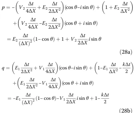
When the amplification factor λ IS equal to λ¼q_p, s= 1−cosθ,θ∈[0, 2] the equations of (28a) and (28b) can be written as:

p¼E2 Δ

t

ΔX2sþ1þV2

Δt

2ΔXisinθ ð30aÞ

q¼−E1 Δ

t

2ΔX2s−V1

Δt

2ΔXisinθþ1− kΔt

2 ð30bÞ

By considering |q|2≤|p|2, it is concluded that the so-lution of the ADI method is stable. The soso-lution stabil-ity of the Barakat-Clark method is unconditionally stable because it has been proven by J. A. Clark and H. Z. Barakat (1966).

A case study

The experimental data of 10 groups are showed in the following table for the least squares method. It considers the process which is mentioned in equation (6a) It de-scribes the least squares method to estimate the initial value of BOD and other parameters (Table 1).

Here it assumes that theh= 0.001 and K’1= 0.1. The

re-sults show K1= 0.3166, L0= 175.5 by going through the

process. The L0value is the initial value of BOD. Therefore,

the water quality model is L(t) = 175.5e−0.3166t. It is a one-dimensional BOD model.

Now, let’s use those other numerical methods including: explicit, implicit, ADI and Barakat-clark to simulate the degradation of contaminants in a section of stream systems. Under natural conditions, the initial value of concentration of pollutants is assumed to be 0 in this stream section. The inflow from the upstream concen-tration of contaminants is 150mg/L. At this point, the equation (8a) is examined. This river section, it is 1000 m long. The water velocity is 17m/s. The diffu-sion rate of pollutantsEis 360. The degradation rate of the pollutant kis 0.15 in this stream. There is a water quality monitor state in every 200 meters. At the same time, the concentration of pollution is consider to be 0 mg/Lat the end of this river, the data is required by the downstream management agencies. Under these con-ditions, the Department of Environmental Protection wants to know the background concentration of con-taminants in this river in order to satisfy the require-ment of those downstream cities. Therefore, by using simulation methods, the concentration of pollutants is estimated using the following methods.

The simulation of explicit method

The water quality modeling can be re-written as a standard form of the explicit method.

Clþ_i 1¼ E Δt ΔX2þV

Δt

2ΔX

Cl_i−1

þ −kΔt−2E Δt ΔX2þ1

Cl_i

þ E Δt ΔX2−V

Δt

2ΔX

Cl_iþ1 ð31aÞ

By substituted the initial value, the solution of equations is as follow,

E Δt

ΔX2¼0:009; V Δt

2ΔX ¼0:0425; kΔt¼0:15

E Δt ΔX2þV

Δt

2ΔX¼0:0515;−kΔt−2E Δt ΔX2þ1 ¼0:832;E Δt

ΔX2−V

Δt

2ΔX¼−0:0335

then,

C1₁¼0:0515C0₀þ0:832C01−0:0335C0₂¼7:725

C1₂¼0:0515C0₁þ0:832C0₂−0:0335C0₃¼0

C1₃¼0:0515C0₂þ0:832C0₃−0:0335C0₄¼0

C1₄¼0:0515C0₃þ0:832C0₄−0:0335C0₅¼0

C2₁¼0:0515C1₀þ0:832C1₁−0:0335C1₂¼14:1522

C2₂¼0:0515C1₁þ0:832C1₂−0:0335C1₃¼0:3978 Table 1 Experimental data of water samples

Time t (day) 1 2 3 4 5 6 7 8 9 10

The simulation of implicit method

Also, the water quality modeling can be re-written as a standard form of the implicit method.

− E Δt

ΔX2þV Δt

2ΔX

Clþ_i−11þ 2E Δt

ΔX2þ1þkΔt

Clþ_i 1

− E Δt

ΔX2−V Δt

2ΔX

Clþ_iþ1₁¼Cl_i

ð32aÞ

Let substitute the value of initial condition. The equa-tions of implicit method is as follow,

E Δt ΔX2þV

Δt

2ΔX ¼0:0515;2E Δt

ΔX2þ1þkΔt

¼1:168;E Δt ΔX2−V

Δt

2ΔX ¼−0:0335

then

1:168 0:0335 0 0

−0:0515 1:168 0:0335 0

0 −0:0515 1:168 0:0335

0 0 −0:0515 1:168

2 6 6 4 3 7 7 5

C1₁ C1₂ C1 3 C1 4 2 6 6 6 4 3 7 7 7 5 ¼ 7:725

0 0 0 2 6 6 4 3 7 7 5

then these C2_{1; C}2_{2; C}2_{3; C}2

4 values can be obtained by using above results.

1:168 0:0335 0 0

−0:0515 1:168 0:0335 0

0 −0:0515 1:168 0:0335

0 0 −0:0515 1:168

2 6 6 4 3 7 7 5 C2 1

C2₂

C2 3

C2₄

2 6 6 6 6 4 3 7 7 7 7 5 ¼

7:725þC1₁ C1

2

C1₃ C1 4 2 6 6 6 4 3 7 7 7 5

The simulation of Barakat-Clark method

The water quality modeling can be re-written as (33a) to (33c), as follows.

Cnþ_i;j1¼ u_inþ_;j1þvnþ_i;j1

=2 ð33cÞ

The parameters areE Δt

ΔX2¼0:009V_ΔΔ_Xt ¼0:0815kΔt¼0:15 . Foruandv; each parameter can be solved as follows:

V Δt ΔX−E

Δt

ΔX2−kΔtþ1¼0:926;E Δt ΔX2−V

Δt ΔX ¼−0:076;1þE Δt

ΔX2¼1:009

u1

1¼

0:926u0_1−0:076u0

2þ0:009u10

1:009 ¼1:338

u1

2¼

0:926u0

2−0:076u03þ0:009u11

1:009 ¼0:012

u1

3¼

0:926u0_3−0:076u0

4þ0:009u12

1:009 ¼0:0001

u1

4¼

0:926u0_4−0:076u0

5þ0:009u13

1:009 ¼0:0000008

u1

3¼

0:926u0₃−0:076u0₄þ0:009u1₂

1:009 ¼0:0001

u1

3¼

0:926u0

3−0:076u04þ0:009u12

1:009 ¼0:0001

u1

4¼

0:926u0

4−0:076u05þ0:009u13

1:009 ¼0:0000008

1þE Δt

ΔX2¼1:009;E Δt

ΔX2¼0:009;−V Δt ΔX−E

Δt ΔX2

−kΔtþ1¼0:756;−E Δt ΔX2−V

Δt

ΔX¼−0:094

1:009 −0:009 0 0

0 1:009 −0:009 0

0 0 1:009 −0:009

0 0 0 1

2 6 6 4 3 7 7 5 v1 1 v1 2 v1₃ v14

2 6 6 4 3 7 7 5¼

−14:1 0 0 0 2 6 6 4 3 7 7 5

The simulation of the ADI Method for two-dimensional water quality modeling

The initial condition of the stream has been given as 50 meters long and 40 meters wide. There is no pollution at the beginning. The contaminants came from upstream. This stream section has 4 monitoring points in every 10 meters. The concentrations of pollutants are 150 mg/L at X direction and 150 mg/L at Y direction. The flow velocity

unþ_i 1¼ V Δt ΔX−E

Δt

ΔX2−kΔtþ1

un_i þ E Δt ΔX2−V

Δt ΔX

un_iþ1þE Δt ΔX2u

nþ1 i−1

=

1þE Δt

ΔX2 ð33aÞ

1þE Δt ΔX2

vlþ_i 1−E Δt ΔX2v

lþ1

iþ1 ¼ −V

Δt ΔX−E

Δt

ΔX2−kΔtþ1

vl_i− E Δt ΔX2þV

Δt ΔX

is 10 m/s in X direction and 5 m/s in Y direction. The dif-fusion rate of pollutantsE1andE2all are equaled to 100.

The degradation rate of the pollutant k is 0.15 in this stream. The department of EPA wants to know this section’s water quality every 10 meter long and every 8 meters wide. Therefore, the simulation methods of pollutants in two-dimensional water quality are tested as follows:

According to the ADI method, the two-dimensional water quality equation can be re-written as follows by considering the first half step as (l= 0.5).

− V2 Δt

2ΔYþE2 Δt ΔY2

C_ilþ_;j−1₁=2þ 2þ2E2 Δt

ΔY2

Cl_iþ_;j1=2

þ V2 Δ

t

2ΔY−E2

Δt ΔY2

Cl_iþ_;jþ1=₁2¼ V1 Δ

t

2ΔXþE1

Δt ΔX2

Cl_i−1;j

þ 2−E1

2Δt ΔX2−kΔt

Cl

i;jþ E1 Δ

t ΔX2−V1 Δ

t

2ΔX

Cl iþ1;j

ð34aÞ

wheni= 1,j= 1, 2, 3, 4

−1:197C0_1;0þ1=2þ3:56C0_1;1þ1=2−0:363C0_1;2þ1=2 ¼0:75C0_0;1þ0:925C0_1;1þ0:25C0_2;1

−1:197C0_1;1þ1=2þ3:56C0_1;2þ1=2−0:363C0_1;3þ1=2 ¼0:75C0_0;2þ0:925C0_1;2þ0:25C0_2;2

−1:197C0_1;2þ1=2þ3:56C0_1;3þ1=2−0:363C0_1;4þ1=2 ¼0:75C0_0;3þ0:925C0_1;3þ0:25C0_2;3

−1:197C0_1;3þ1=2þ3:56C0_1;4þ1=2−0:363C0_1;5þ1=2 ¼0:75C0_0;4þ0:925C0_1;4þ0:25C0_2;4

There C0₁þ_;11=2:C0₁þ_;21=2;C0₁þ_;31=2;C0₁þ_;41=2, they can be ob-tained by above equations. Then, it substitutedi= 2, j= 1, 2, 3, 4, the equation (34a) can be written as following,

−1:197C0_2;0þ1=2þ3:56C0_2;1þ1=2−0:363C0_2;2þ1=2 ¼0:75C0_1;1þ0:925C0_2;1þ0:25C0_3;1

−1:197C0_2;1þ1=2þ3:56C0_2;2þ1=2−0:363C0_2;3þ1=2 ¼0:75C0_1;2þ0:925C0_2;2þ0:25C0_3;2

−1:197C0_2;2þ1=2þ3:56C0_2;3þ1=2−0:363C0_2;4þ1=2 ¼0:75C0_1;3þ0:925C0_2;3þ0:25C0_3;3

−1:197C0_2;3þ1=2þ3:56C0_2;4þ1=2−0:363C0_2;5þ1=2 ¼0:75C0_1;4þ0:925C0_2;4þ0:25C0_3;4

C0₂þ_;11=2:C0₂þ_;21=2;C0₂þ_;31=2;C0₂þ_;41=2, they can be obtained by above equations. Similarly, let substitute i= 3, 4, and j= 1, 2, 3, 4.

The second half of the ADI method is based on the results of the first step. By using i= 1,j= 1, 2, 3, 4, the equation (34a) can be written as,

−0:0165C1_0;1þ2:218C1_1;1−0:0015C1_2;1 ¼50:5C0_1;0þ1=2−98C_1;10þ1=2−49:5C0_1;2þ1=2

−0:0165C1_1;1þ2:218C12;1−0:0015C1_3;1 ¼50:5C0_2;0þ1=2−98C_2;10þ1=2−49:5C0_2;2þ1=2

−0:0165C1_2;1þ2:218C1_3;1−0:0015C1_4;1 ¼50:5C0_3;0þ1=2−98C_3;10þ1=2−49:5C0_3;2þ1=2

−0:0165C1_3;1þ2:218C1_4;1−0:0015C1_5;1 ¼50:5C0_4;0þ1=2−98C_4;10þ1=2−49:5C0_4;2þ1=2

These C1_1;1:C1_2;1;C1_3;1;C1_4;1 can be solved using above equations. Substituting j= 1, i= 1, 2, 3, 4, the equation (34a) can be written as,

− E1 Δ

t ΔX2þV1

Δt ΔX

Cl_iþ₋₁1_;jþ 2þE1

2Δt ΔX2þkΔt

C_ilþ_;j1

− E1 Δ

t ΔX2−V1 Δ

t

2ΔX

Cl_iþþ1_1;j¼ E2 Δ

t

ΔY2þV2 Δ

t

2ΔY

Cl_iþ_;j−1₁=2

þ 2−E2 Δ

t ΔY2

Cl_iþ_;j1=2þ E2 Δ

t ΔY2−V2 Δ

t

2ΔY

Cl_i;þ_jþ1=₁2

ð34bÞ

−0:75C1_0;1þ3:075C1_1;1−0:25C1_2;1

¼1:197C0_1;0þ1=2þ1:22C0_1;1þ1=2þ0:363C0_1;2þ1=2

−0:75C1_1;1þ3:075C12;1−0:25C1_3;1

¼1:197C0_2;0þ1=2þ1:22C0_2;1þ1=2þ0:363C0_2;2þ1=2

−0:75C1_2;1þ3:075C1_3;1−0:25C1_4;1

¼1:197C0_3;0þ1=2þ1:22C0_3;1þ1=2þ0:363C0_3;2þ1=2

−0:75C1_3;1þ3:075C1_4;1−0:25C1_5;1

¼1:197C0_4;0þ1=2þ1:22C0_4;1þ1=2þ0:363C0_4;2þ1=2

Let substitutej= 2,i= 1, 2, 3, 4, the equation (34a) can be written as,

−0:75C1_0;2þ3:075C1_1;2−0:25C1_2;2

¼1:197C0_1;1þ1=2þ1:22C0_1;2þ1=2þ0:363C0_1;3þ1=2

−0:75C1_1;2þ3:075C1_2;2−0:25C1_3;2

¼1:197C0_2;1þ1=2þ1:22C0_2;2þ1=2þ0:363C0_2;3þ1=2

−0:75C1_2;2þ3:075C1_3;2−0:25C1_4;2

−0:75C1

3;2þ3:075C14;2−0:25C15;2

¼1:197C0_4;1þ1=2þ1:22C0_4;2þ1=2þ0:363C0_4;3þ1=2

Thus, C1_1;2:C1_2;2;C1_3;2;C1_4;2 can be obtained by above equations. Similarly, the other C value is calculated by substitutingi=3, 4.

The simulation of Barakat-Clark method for two-dimensional modeling

This model is similar to the one-dimensional water quality modeling. If it considers the two different directions (x,y). The group of equations can be written as,

ulþi;j1¼

V1Δ t

ΔXþV2

Δt

ΔY−E1

Δt

ΔX2−E2

Δt

ΔY2−kΔtþ1

ul i;j

þ E1 Δ t

ΔX2−V1 Δ t

ΔX

ul

iþ1;jþ E2 Δ t

ΔY2−V2Δ t

ΔY

ul i;jþ1

þE1 Δ t

ΔX2u

lþ1 i−1;jþE2 Δ

t

ΔY2u

lþ1 i;j−1 =

1þE1 Δ t

ΔX2þE2 Δt

ΔY2

ð35aÞ

in this case, theuvalues are as follows

u1

1;1¼ 0:312u01;1þ0:25u02;1þ0:363u01;2þ0:5u01;1þ0:78u11;0

=2:28

¼84:21

u1

1;2¼ 0:312u01;2þ0:25u02;2þ0:363u01;3þ0:5u01;2þ0:78u11;1

=2:28

¼61:7

u11;3¼ 0:312u 0

1;3þ0:25u 0

2;3þ0:363u 0 1;4þ0:5u

1

0;3þ0:78u 1 1;2

=2:28

¼54

u1

1;4¼ 0:312u01;4þ0:25u02;4þ0:363u01;5þ0:5u01;4þ0:78u11;3

=2:28

¼51:37

u12;1¼ 0:312u 0

2;1þ0:25u 0

3;1þ0:363u 0 2;2þ0:5u

1

1;1þ0:78u 1 2;0

=2:28

¼69:783

u1

2;2¼ 0:312u02;2þ0:25u03;2þ0:363u02;3þ0:5u11;2þ0:78u12;1

=2:28

¼37:4

u12;3¼ 0:312u 0

2;3þ0:25u 0

3;3þ0:363u 0 2;4þ0:5u

1

1;3þ0:78u 1 2;2

=2:28

¼24:64

u12;4¼ 0:312u 0

2;4þ0:25u 0

3;4þ0:363u 0 2;5þ0:5u

1

1;4þ0:78u 1 2;3

=2:28

¼19:695

The rest ofuvalues can be calculated by substituting i=3, 4.

E1 Δt

ΔX2v lþ1

iþ1;jþE2 Δt

ΔY2v lþ1

i;jþ1− 1þE1 Δt

ΔX2þE2

Δt ΔY2

vliþ;j1

¼ V1_ΔXΔt þV2_ΔYΔt þE1 Δt

ΔX2þE2

Δt

ΔY2þkΔt−1

vl i;j

− V1_ΔXΔt þE1 Δt

ΔX2

vl_i−1;j− V2_ΔYΔt þE2 Δt

ΔY2

vl_i;j−1

ð35bÞ

Thevvalues are calculated by the following process:

0:5v1_2;1þ0:78v1_1;2−1:022v1_1;1

¼1:022v0_1;1−0:75v_0;10 −1:197v0_1;0¼−292:05

0:5v1_2;2þ0:78v1_1;3−1:022v1_1;2

¼1:022v0_1;2−0:75v_0;20 −1:197v0_1;1¼−112:5

0:5v1_2;3þ0:78v1_1;4−1:022v1_1;3

¼1:022v0_1;3−0:75v_0;30 −1:197v0_1;2¼−112:5

0:5v1_2;4þ0:78v1_1;5−1:022v1_1;4

¼1:022v0_1;4−0:75v_0;40 −1:197v0_1;3¼−112:5

0:5v1_3;1þ0:78v1_2;2−1:022v1_2;1

¼1:022v02;1−0:75v1;1−0 1:197v0_2;0¼−179:55

0:5v1_3;2þ0:78v1_2;3−1:022v1_2;2

¼1:022v02;2−0:75v1;2−0 1:197v0_2;1¼−112:5

0:5v1_3;3þ0:78v12;4−1:022v1_2;3

¼1:022v02;3−0:75v01;3−1:197v0_2;2¼0

0:5v1_3;4þ0:78v12;5−1:022v1_2;4

¼1:022v02;4−0:75v01;4−1:197v0_2;3¼0

When these values of u and v were calculated, the final solution of the Barakart-Clark method can be obtained by using average value of those two matrixes.

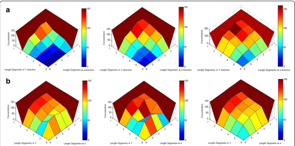
Results and discussion

it may have been caused by a large space of x or y. However, under same steps and space of x and y, the Barakat-Clark method obtained the better accuracy results. The Barakat-Clark method uses less computing time to get those results. This method has the advantage of solving the three dimensions time-dependent equations which is not convenient for ADI method.

The data results (Tables 2, 3, 4, 5 and 6) of the above equations show the detailed numerical solutions of the water quality modelling process. The findings in Table 4 show smoother curves of water quality because of different method. Although the explicit method obtained stable results in this case, whenXvalue is changed to a smaller value, the results will be extremely unstable. It means that the stability of the solution is depends on the size

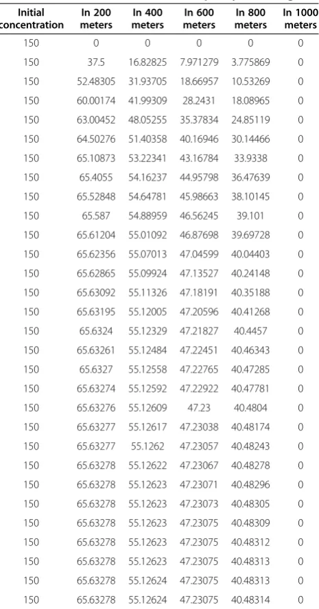
of grid for explicit method. It is obvious to see that the solution of the Barakat-Clark method is more stable, even though the size of the grid was changed. This is because the Barakat-Clark numerical method has been considered average values or mean values of implicit and explicit data. Therefore, the Barakat-Clark methodology is more accurate than others in the case of the water quality simulation process.

Conclusions

In this study, the finite difference numerical methods are applied to the water quality modeling processes. They simulate the concentration process of pollutants in hydrological systems. As one of the existing numerical methods, the Barakat-Clark has obtained higher accuracy Figure 1The results of explicit, implicit and barakat-clark methods for 1-D water quality modeling.

results with stability than the other methods. By compar-ing the solution of Barakat-Clark method with the other numerical methods, its results better reflect the reality of the simulation without oversimplify solving the process. The water quality modeling process, which estimates the real world conditions, can be effectively solved by means of the Barakat-Clark method. It enables the managers of water authorities to know the concentration of pollution in surface water systems and to conveniently use those so-lutions as a reference in their hydrological systems. Conse-quently, the accurate of water quality simulation processes can be enhanced. The results of the case study indicates that the solution of Barakat-Clark method has proved that

this method is better by comparison than the others for water quality modeling. Solutions of the numerical method actually reflect a compromise between the finite difference method and requirement of accuracy.

In the real world, administrators of water management agencies are paying a high price for water quality to guarantee the safe conditions of environmental water. This means that authorities desire to accurate monitor-ing data to determine the stream or river situations. This may cause a higher economic cost. However, simu-lation values of water quality are reliable within the Barakat-Clark method. Its advantages have been clearly shown in the above case study. It shows that the results

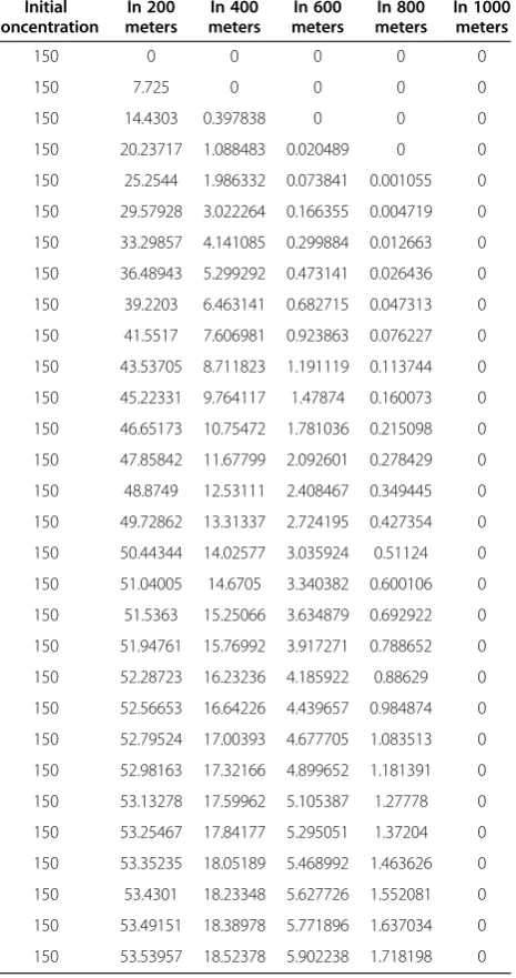
Table 2 Concentration results of pollutants using the explicit method for 1-D water quality modeling

Initial concentration

In 200 meters

In 400 meters

In 600 meters

In 800 meters

In 1000 meters

150 0 0 0 0 0

150 7.725 0 0 0 0

150 14.4303 0.397838 0 0 0

150 20.23717 1.088483 0.020489 0 0

150 25.2544 1.986332 0.073841 0.001055 0

150 29.57928 3.022264 0.166355 0.004719 0

150 33.29857 4.141085 0.299884 0.012663 0

150 36.48943 5.299292 0.473141 0.026436 0

150 39.2203 6.463141 0.682715 0.047313 0

150 41.5517 7.606981 0.923863 0.076227 0

150 43.53705 8.711823 1.191119 0.113744 0

150 45.22331 9.764117 1.47874 0.160073 0

150 46.65173 10.75472 1.781036 0.215098 0

150 47.85842 11.67799 2.092601 0.278429 0

150 48.8749 12.53111 2.408467 0.349445 0

150 49.72862 13.31337 2.724195 0.427354 0

150 50.44344 14.02577 3.035924 0.51124 0

150 51.04005 14.6705 3.340382 0.600106 0

150 51.5363 15.25066 3.634879 0.692922 0

150 51.94761 15.76992 3.917271 0.788652 0

150 52.28723 16.23236 4.185922 0.88629 0

150 52.56653 16.64226 4.439657 0.984874 0

150 52.79524 17.00393 4.677705 1.083513 0

150 52.98163 17.32166 4.899652 1.181391 0

150 53.13278 17.59962 5.105387 1.27778 0

150 53.25467 17.84177 5.295051 1.37204 0

150 53.35235 18.05189 5.468992 1.463626 0

150 53.4301 18.23348 5.627726 1.552081 0

150 53.49151 18.38978 5.771896 1.637034 0

150 53.53957 18.52378 5.902238 1.718198 0

Table 3 Concentration results of pollutants using the implicit method for 1-D water quality modeling

Initial concentration

In 200 meters

In 400 meters

In 600 meters

In 800 meters

In 1000 meters

150 0 0 0 0 0

150 6.605527 0.290887 0.01281 0.000565 0

150 12.24669 0.787725 0.045628 0.002495 0

150 17.05822 1.423646 0.101648 0.006618 0

150 21.15694 2.146537 0.181281 0.01366 0

150 24.64405 2.916286 0.283099 0.024177 0

150 27.60703 3.70248 0.404526 0.038536 0

150 30.12146 4.482505 0.542353 0.056907 0

150 32.2525 5.239974 0.693113 0.079283 0

150 34.05628 5.96343 0.853335 0.105505 0

150 35.58104 6.645285 1.019722 0.135292 0

150 36.86826 7.280959 1.189259 0.168269 0

150 37.95349 7.868175 1.359277 0.204 0

150 38.86719 8.406391 1.527482 0.242008 0

150 39.63541 8.896348 1.691955 0.281801 0

150 40.28042 9.339706 1.851141 0.322889 0

150 40.82121 9.738758 2.003824 0.3648 0

150 41.27396 10.09621 2.149094 0.407088 0

150 41.65245 10.415 2.286313 0.449343 0

150 41.96837 10.69817 2.41508 0.491198 0

150 42.23167 10.94878 2.535196 0.53233 0

150 42.45075 11.1698 2.64663 0.572458 0

150 42.63275 11.36411 2.749488 0.61135 0

150 42.78369 11.53442 2.843985 0.648814 0

150 42.90865 11.68326 2.930424 0.684701 0

150 43.01191 11.81298 3.009169 0.718899 0

150 43.09709 11.92575 3.08063 0.751328 0

150 43.16721 12.02354 3.145246 0.781942 0

150 43.22482 12.10814 3.203473 0.81072 0

of the Barakat-Clark method is more reliable and more accurate with process stability. On the other hand, other numerical methods such as ADI method produced a different results under same circumstances. Therefore, the Barakat-Clark method can be considered as a better finite method in the 2-D water modeling system, and this paper is the first attempt to compare the Barakat-Clark 2-D method with other multiple numerical algorithms in the water quality modeling process. From the above applica-tions, it is obvious that the Barakat-Clark method shares higher stability results with the same environmental condi-tions. However, in this study, the boundary conditions have been pre-defined. Therefore, further studies of this method have to correspond to the variation of boundary conditions in real world. Finally, this the 2-D Barakat-Clark method well reflects the accuracy of simulation process, and thus, it can provide an exact reference for water quality modeling in hydrological systems.

Competing interests

The authors declare that they have no competing interests.

Authors’contributions

Author LJ composed this paper, and others have revised it many times for publication. All authors read and approved the final manuscript.

Acknowledgements

This research was supported by the Program for Innovative Research Team (IRT1127), the Natural Science and Engineering Research Council of Canada, the MOE Key Project Program (311013), Natural Science Foundation of China (51109181) and the Scientific Research fund project (XKJJ201105) of Xiamen University of Technology. The writers are very grateful to the editor and the anonymous reviewers for their insightful comments and suggestions.

Author details

1

College of Environmental Science and Engineering, Xiamen University of Technology, Xiamen, Fujian Province 361024, China.2_{College of Applied} Mathematics, Xiamen University of Technology, Xiamen, Fujian Province 361024, China.

Received: 29 November 2013 Accepted: 12 December 2013 Published: 23 December 2013

References

Barakat HZ, Clark JA (1966) On the solution of the diffusion equations by numerical methods. J Heat Tran 11:421–427

Cash JR (2003) Efficient numerical methods for the solution of stiff initial-value problems and differential algebraic equations. Proc R Soc Lond 459:797–815 Table 4 Concentration results of pollutants using the

Barakat-Clark method for 1-D water quality modeling Initial

concentration

In 200 meters

In 400 meters

In 600 meters

In 800 meters

In 1000 meters

150 0 0 0 0 0

150 37.5 16.82825 7.971279 3.775869 0

150 52.48305 31.93705 18.66957 10.53269 0

150 60.00174 41.99309 28.2431 18.08965 0

150 63.00452 48.05255 35.37834 24.85119 0

150 64.50276 51.40358 40.16946 30.14466 0

150 65.10873 53.22341 43.16784 33.9338 0

150 65.4055 54.16237 44.95798 36.47639 0

150 65.52848 54.64781 45.98663 38.10145 0

150 65.587 54.88959 46.56245 39.101 0

150 65.61204 55.01092 46.87698 39.69728 0

150 65.62356 55.07013 47.04599 40.04403 0

150 65.62865 55.09924 47.13527 40.24148 0

150 65.63092 55.11326 47.18191 40.35188 0

150 65.63195 55.12005 47.20596 40.41268 0

150 65.6324 55.12329 47.21827 40.4457 0

150 65.63261 55.12484 47.22451 40.46343 0

150 65.6327 55.12558 47.22765 40.47285 0

150 65.63274 55.12592 47.22922 40.47781 0

150 65.63276 55.12609 47.23 40.4804 0

150 65.63277 55.12617 47.23038 40.48174 0

150 65.63277 55.1262 47.23057 40.48243 0

150 65.63278 55.12622 47.23067 40.48278 0

150 65.63278 55.12623 47.23071 40.48296 0

150 65.63278 55.12623 47.23073 40.48305 0

150 65.63278 55.12623 47.23075 40.48309 0

150 65.63278 55.12623 47.23075 40.48312 0

150 65.63278 55.12623 47.23075 40.48313 0

150 65.63278 55.12624 47.23075 40.48313 0

150 65.63278 55.12624 47.23075 40.48314 0

Table 5 Results of ADI method for 2-D water quality modeling in final time (x/ydirection)

Initial concentration

In 200 meters

In 400 meters

In 600 meters

In 800 meters

In 1000 meters

150 150 150 150 150 150

150 124.9046 133.1181 96.9082 77.9531 0

150 117.1522 96.6831 60.7363 54.3516 0

150 102.0593 74.4782 34.3785 31.6676 0

150 80.1334 54.9374 21.4405 13.6352 0

150 0 0 0 0 0

Table 6 Results of Barakat-Clark method for 2-D water quality modeling in final time (x/ydirection)

Initial concentration

In 200 meters

In 400 meters

In 600 meters

In 800 meters

In 1000 meters

150 150 150 150 150 150

150 119.8325 127.1802 125.1696 101.3011 0

150 107.2249 110.1196 104.7594 77.7571 0

150 101.0918 99.1784 90.7855 64.4765 0

150 97.8035 92.4481 81.7728 56.4511 0

Christie MA, Bond DJ (1987) Detailed simulation of unstable processes in miscible flooding. Reserv Eng 2:514–522

Davis HT (1962) Induction to nonlinear differential and integral equations. Dover, New York

Evans DJ, Abdullah AR (1985) A new explicit method for diffusion-convection equation. Comp Maths Applis 11:145–154

Hoffman J (1992) Numerical methods for engineers and scientists. McGraw-Hill, New York

Kellogg RB (1964) An alternating direction method for operator equations. SIAM 12:848–854

Liu WC, Jantai K, Albert Y (2005) Modelling hydrodynamics and water quality in the separation waterway of the Yulin offshore industrial park, Tainwan. Environ Model Softw 20:309–328

Moiianty RK (2004) An unconditionally stable difference scheme for the one-space-dimensional linear hyperbolic equation. Appl Math Lett Letters 17:101–105 Munavalli GR, Mohan Kumar MS (2004) Modified Lagrangian method for

modeling water quality in distribution systems. Water Res 38:973–2988 Na TY (1979) Computational methods in engineering boundary value problem.

Academic Press, New York

Noye BJ, Hayman KJ (1992) Explicit two-level finite difference methods for the two-dimensional diffusion equation. J Comput Math 42:223–236 Richard JB, Robert S (1997) Expanded stability through higher accuracy for

time-centered advection schemes. American Meteorological Society, Springer, Herdelberg, p 6

Rudi R, Matjaz C (1997) Hydrodynamic and water quality modeling: An experience. Ecol Model 101:195–207

Shampine LF, Gear CW (1979) A user’s view of solving stiff ordinary differential equations. SIAM Rev 21:1

Shawgfeh N, Kaya D (2004) Comparing numerical methods for the solutions of systems of ordinary differential equations. Appl Math Lett 17:323–328 Stasa FL (1985) Applied finite element analysis for engineers. Holt Rinehart and

Winston, New York

Taylor JR (1982) An introduction to error analysis. Mill Valley, CA

Timo T, Sampsa K, Ville K, Matthieu M, Peng CY (2013) Water quality analysis using an inexpensive device and a mobile phone. Env Syst Res 2:9 Walter MG (2006) Use of distribution system water quality models in support of water

security. Security of Water Supply System, Springer, Heidelerg, pp 39–50

doi:10.1186/2193-2697-2-11

Cite this article as:Jinet al.:A 2-D Barakat-Clark finite difference numerical method and its comparison for water quality simulation modeling. Environmental Systems Research20132:11.

Submit your manuscript to a

journal and benefi t from:

7Convenient online submission 7Rigorous peer review

7Immediate publication on acceptance 7Open access: articles freely available online 7High visibility within the fi eld

7Retaining the copyright to your article