A brief review on the convergence to steady state solutions of Euler equations with high-order WENO schemes

R E V I E W

Open Access

A brief review on the convergence to

steady state solutions of Euler equations

with high-order WENO schemes

Shuhai Zhang

, Jun Zhu

and Chi-Wang Shu

*Correspondence: [email protected] 3_{Division of Applied Mathematics,} Brown University, Providence, RI 02912, USA

Full list of author information is available at the end of the article

Abstract

Weighted essentially non-oscillatory (WENO) schemes are a class of high-order shock capturing schemes which have been designed and applied to solve many fluid dynamics problems to study the detailed flow structures and their evolutions. However, like many other high-order shock capturing schemes, WENO schemes also suffer from the problem that it can not easily converge to a steady state solution if there is a strong shock wave. This is a long-standing difficulty for high-order shock capturing schemes. In recent years, this non-convergence problem has been studied extensively for WENO schemes. Numerical tests show that the key reason of the non-convergence to steady state is the slight post shock oscillations, which are at the small local truncation error level but prevent the residue to settle down to machine zero. Several strategies have been proposed to reduce these slight post shock oscillations, including the design of new smoothness indicators for the fifth-order WENO scheme, the development of a high-order weighted interpolation in the procedure of the local characteristic projection for WENO schemes of higher order of accuracy, and the design of a new type of WENO schemes. With these strategies, the convergence to steady states is improved significantly. Moreover, the strategies are applicable to other types of weighted schemes. In this paper, we give a brief review on the topic of convergence to steady state solutions for WENO schemes applied to Euler equations.

Keywords: WENO scheme, Convergence, Steady state solution, Smoothness indicator, WENO compact scheme

1 Introduction

Over the past few decades, computational fluid dynamics (CFD) has become an impor-tant tool to study flow structures and aerodynamic forces through solving the compress-ible Euler or Navier-Stokes equations. Steady states are common in aerodynamics in which the non-viscous flow fields are governed by the following Euler equations:

d

i=1

∂Fi(U) ∂xi =

0, (1)

whereUis the vector of the conserved variables,Fi(U)is the nonlinear flux function in

the i-th direction, anddis the spatial dimension. Among numerous methods to obtain a numerical solution of (1), one possible choice is to solve the following unsteady Euler equations by a time marching method:

∂U

∂t +

d

i=1

∂Fi(U) ∂xi =

0. (2)

When the time derivative or the residue of the unsteady Euler Eq. (2) becomes small enough (ideally at or close to machine zero), a numerical solution of the steady state Eq. (1) is obtained.

Shock waves are a key structure of supersonic flows. Across a shock wave, the physi-cal variables are discontinuous. In the history of CFD, the design of numeriphysi-cal schemes that can capture shock waves well has been a tough problem. Many classical numeri-cal schemes would produce severe spurious oscillations near shock waves. To eliminate or reduce such severe spurious oscillations, shock capturing schemes were carefully designed. The most popular shock capturing schemes include total variation diminishing (TVD) schemes [1], essentially non-oscillatory (ENO) schemes [2–4], and weighted ENO (WENO) schemes [5–7]. The TVD schemes were proposed by Harten [1]. Through the application of suitable limiters, TVD schemes can achieve the total variation diminish-ing property, which makes it very popular in the simulation of supersonic flows includdiminish-ing strong shock waves. The non-oscillatory and no-free-parameter dissipation (NND) differ-ence scheme, proposed by Zhang et al. [8–10], is a special type of TVD schemes. Through analyzing the evolution of the numerical error for Navier-Stokes equations, Zhang [8] found the relationship between the coefficients of the modified equation and the spu-rious oscillation at both sides of the shock waves. Then, he proposed the NND scheme through controlling the oscillation around the shock waves by a limiter. It was proved that the NND scheme has the TVD property [9]. However, all TVD schemes degenerate to first-order accuracy near smooth extrema due to the application of the TVD limiters [11]. ENO schemes are a type of high-order shock capturing schemes that was proposed by Harten et al. [2]. Instead of using a fixed stencil to reconstruct the numerical fluxes, the locally smoothest stencil among several candidates is used in ENO schemes. The smooth-ness of a stencil is measured by the corresponding divided differences. The ENO scheme has the property of being self similar and parameter-free, uniformly high-order accurate and very robust with essentially no oscillations near shock waves. However, there are still several drawbacks that can be improved. For example, the stencil might be changed even by a round-off error perturbation near zeroes of the solution and its derivatives. This may result in a loss of accuracy of the scheme when it is applied to a hyperbolic PDE. In the process of choosing the stencil, several candidate stencils are considered, but only one of them, the so called smoothest stencil in some sense, is actually used in the recon-struction of the numerical flux. This means that ENO schemes could not achieve the optimal accuracy order associated with the combined set of all the cells considered in the selection.

WENO schemes [5–7] are an extension of the ENO schemes. Instead of using only the smoothest stencil, a WENO scheme uses all candidate stencils through a convex combina-tion to approximate the fluxes. The accuracy is improved to the optimal order in smooth regions while the essentially non-oscillatory property near discontinuities is maintained. WENO schemes have been extensively applied in many areas including CFD.

the residue can not settle down to a satisfactory value (ideally machine zero) but would hang at a relatively high local truncation error level. The reason is that there are slight spurious oscillations in the neighborhood region of the shock waves. For TVD schemes, because of the use of limiters, the numerical fluxes of the TVD schemes are less smooth. This makes them difficult to converge to steady states. In ENO schemes, the numerical flux is not smooth either when the stencil pattern changes at neighboring points, caus-ing difficulty in convergence to steady states as well. Even though the numerical flux of WENO schemes is smoother than that of ENO schemes, the WENO schemes could also suffer from the same problem, especially for multi-dimensional flows with strong shocks.

In recent years, the issue of the lack of convergence to steady state solutions for WENO schemes is studied extensively [12–15]. In [15], Zhang and Shu studied the mecha-nism of the non-convergence of the fifth-order WENO scheme, and found that there is a relationship between the smoothness indicators and the post-shock oscillations. A new smoothness indicator was proposed for the fifth-order WENO scheme. With this new smoothness indicator, the residue can settle down to machine zero for many test problems. In [13], Zhang et al. studied the non-convergence of WENO schemes of higher orders of accuracy. They found that there is some relationship between the local characteristic projection and the appearance of post shock oscillations. A high-order upwind-biased weighted interpolation is proposed to obtain the physical values in the middle of two grid points when computing the Jacobian matrix and its eigenvectors dur-ing the local characteristic projection. These strategies can be applied to other types of weighted schemes as well [12,14]. In more recent years, Zhu et al. [16–22] proposed new types of WENO schemes with the application of a series of unequal-sized spatial stencils. Such new WENO schemes have very nice convergence property to steady state solutions. In this paper, we give a brief review on the convergence to steady state solutions of WENO schemes. The paper is organized as follows. In Section2, we give an overview of the WENO methodology. The mechanism of non-convergence of WENO schemes to steady state solutions is explained in Section3. Two techniques to improve the conver-gence property of WENO schemes are presented in Section4. Section5describes the application of these techniques for improving steady state convergence to other types of weighted schemes including the fast sweeping WENO schemes and weighted compact schemes. Section6 describes the new type of WENO schemes proposed by Zhu et al. [16,19], emphasizing its nice property in steady state convergence. Section7contains our perspectives and discussions on the problem of steady state convergence for high-order WENO schemes.

2 Methodology of the WENO schemes

In this section, we give a brief overview of the finite difference WENO schemes includ-ing the numerical fluxes, the smoothness indicators, and the discretization of the time derivative.

2.1 Numerical fluxes of the WENO schemes

We use the one-dimensional scalar conservative law

as an example to explain the reconstruction of the numerical fluxes for finite difference WENO schemes. In general, the physical flux f(u) can be split into two parts, either globally or locally,

f(u)=f+(u)+f−(u) (4)

where, df_du+(u) ≥ 0 and df_du−(u) ≤ 0. The Lax-Friedrichs flux splitting is the simplest and commonly used flux splitting method, which is given by

f±(u)= 1

2(f(u)±αu), (5)

whereα=maxf(u)with the maximum taken over some relevant range ofu.

For simplicity, we assumef(u) ≥ 0 in (3) to show the WENO procedure for approxi-mating the fluxf+(u). The formulae for the approximation off−(u)are symmetric with respect to the middle point x_i+1

2. The computational domain [xL,xR] is divided to a

uniform mesh ofx=xj+1−xj=const.

For finite difference WENO schemes, the spatial derivativef(u)xat the pointx=xiin

(3) is approximated by a conservative finite difference formula

∂ui ∂t = −

1

x

ˆ

f_i+1

2 − ˆfi−12

=L(u)i (6)

where the numerical flux ˆf_i+1

2 approximates hi+12 to high-order accuracy, with h(x)

defined by Shu and Osher in [4] through the indirect requirement

f(u(x))= 1

x

_x+x

2

x−x

2

h(ξ)dξ. (7)

In a (2r−1)-point upwind-biased stencilS2r−1 = {xi−r+1, ...,xi+r−1}for the middle

pointx_i+1

2, a(2r−1)-th order numerical flux can be reconstructed as follows:

ˆ

f_i+1

2 =q 2r−1_(f

i−r+1, ...,fi+r−1). (8)

The big stencilS2r−1can be divided intorsub-stencils

S_k2r−1= {xi+k−r+1,xi+k−r+2, ...,xi+k}, k=0, 1, ...,r−1.

In each of these sub-stencils, anr-th order reconstruction can be obtained

ˆ

f(k)

i+1

2 =

q_kr(f_i+k−r+1, ...,f_i+k), (9)

where

qr_k(g0, ...,gr−1)= r−1

l=0

ar_k,lgl.

Here,ar_k,l, 0≤k,l≤r−1, are constant coefficients.

Using theserstencils as candidates, the ENO scheme chooses the smoothest sub-stencil to approximate the flux. The obtained numerical flux is onlyr-th order accurate which is given by (9) with the chosen k. In fact, if all of these sub-stencils are used, the numerical flux can achieve the optimal accuracy order 2r− 1, which is given by (8). Through simple derivation, one can find thatq2r−1can also be obtained by a linear combination offˆ(k)

i+1₂

q2r−1(fi−r+1, ...,fi+r−1)= r−1

k=0

Heredk=drk(k=0, ..,r−1)are constant coefficients, which are called the linear weights.

The formula (10) is the same as the formula (8). It results in a linear scheme, which can not be used to compute the flow field with strong discontinuities. Through introducing the nonlinear weightsωk (k = 0, ...,r−1) to replace the linear weights, Liu et al. [7]

proposed the WENO scheme with the numerical flux as follows:

ˆ

f_iWENO₊1

2 =

r−1

k=0

ωkfˆ_i(₊k)1 2

. (11)

The nonlinear weightsωkare defined by

ωk = _α αk

0+α1+...+αr−1

, (12)

where

αk =

dk

(ε+ISk)p

, k=0, 1, ...,r−1. (13)

Hereεis a small positive number which is introduced to avoid the denominator to become zero andpis an empirical parameter. Usually we takeε = 10−6 andp = 2.ISk is the

smoothness indicator to measure the smoothness of the flux function in thek-th sub-stencil. The smoothness indicator is not unique. The choice of the smoothness indicator can have influence over the accuracy and the convergence towards the steady state [6,7,

15,23]. WENO schemes can achieve optimal order of accuracy in smooth regions while the essentially non-oscillatory property is maintained in the region near discontinuities. In [7], Liu et al. used the undivided differences to compute the smoothness indicator

ISk =

r−1

l=1 r−l

i=1

f[j+k+i−r,l]2

r−l . (14)

Heref[j,l] are thel-th order undivided differences:

f[j, 0]=fj, f[j,l]=f[j+1,l−1]−f[j,l−1] , l=1, ...,r−1. (15)

Using this smoothness indicator, the accuracy order of the WENO scheme is onlyr+1, not the optimal 2r−1. Jiang and Shu [6] introduced the following smoothness indicator:

IS_k =

r−1

l=1

x_i+1 2

x_i−1 2

x2l−1 ∂

l_fk_(x)

∂l_x

2

dx, (16)

wherefk(x)is the reconstruction polynomial based on the sub-stencilS2_kr−1. With this smoothness indicator, the WENO scheme can achieve the optimal accuracy order.

a. The fifth-order WENO scheme

The fifth-order WENO scheme (r = 3) has been applied most extensively (among all WENO schemes) in the computation of aerodynamics and in scientific computation of many other areas after it was developed by Jiang and Shu [6]. The three third-order numerical fluxes in the three sub-stencils are

ˆ

f_j0_+1/2= 1₃fj−2− 7₆fj−1+ 11₆fj,

ˆ

f_j1_+1/2= −1₆fj−1+5₆fj+1₃fj+1,

ˆ

f_j2_+1/2= 1₃fj+ 5₆fj+1− 1₆fj+2.

(17)

The linear weights are

d0=

1

10, d1= 6

10, d2= 3

and the smoothness indicators are

IS0= 13₁₂

fj−2−2fj−1+fj

2₊1 4

fj−2−4fj−1+3fj

2

,

IS1= 13₁₂

fj−1−2fj+fj+1

2

+1 4

fj−1−fj+1

2

,

IS2= 13₁₂

fj−2fj+1+fj+2

2₊1 4

3fj−4fj+1+fj+2

2

.

(19)

Henrick et al. [23] noticed that the WENO scheme with the smoothness indicator (19) may lose accuracy at certain smooth extrema. To recover the accuracy order at these smooth extrema, they introduced a mapping function:

gk(ω)=

ωdk+d_k2−3dkω+ω2

d2_k+(1−2dk)ω

, (20)

wheredk ∈ (0, 1] andk = 0, 1, 2. The functiongk(ω)is monotonically increasing with

a finite slope andgk(0) = 0,gk(1) = 1,gk(dk) = dk,g_k(dk) = 0, andg_k(dk) = 0. The

mapped weights are given by:

ω∗k=gk(ωk), ωMk =

ω∗ k ω∗

1+ω∗2+ω3∗

, (21)

where ωk are computed by (12) and (19). This mapped WENO scheme can improve

accuracy at smooth extrema. We refer to [23] for more details.

b. Seventh-order WENO scheme

In the case ofr=4, the seventh-order WENO scheme was obtained by Balsara and Shu [5]. The four fourth-order numerical fluxes from the four sub-stencils are

ˆ

f0

i+1₂ = − 1

4fi−3+ 13₁₂fi−2−23₁₂fi−1+25₁₂fi,

ˆ

f1

i+1

2 =

1

12fi−2− 125fi−1+ 1312fi+14fi+1,

ˆ

f2

i+1

2 = −

1

12fi−1+127fi+ 127fi+1− 121fi+2,

ˆ

f3

i+1₂ = 1 4fi+

13 12fi+1−

5 12fi+2+

1 12fi+3.

(22)

The linear weights are given by

d0=

1

35, d1= 13

35, d2= 18

35, d3= 4

35, (23)

and the smoothness indicators are

IS0= fi−3(547fi−3−3882fi−2+4642fi−1−1854fi)

+fi−2(7043fi−2−17246fi−1+7042fi)

+fi−1(11003fi−1−9402fi)+2107fi2,

IS1= fi−2(267fi−2−1642fi−1+1602fi−494fi+1)

+fi−1(2843fi−1−5966fi+1922fi+1)

+fi(3443fi−2522fi+1)+547f_i2₊₁,

IS2= fi−1(547fi−1−2522fi+1922fi+1−494fi+2)

+fi(3443fi−5966fi+1+1602fi+2)

+fi+1(2843fi+1−1642fi+2)+267fi2+2,

IS3= fi(2107fi−9402fi+1+7042fi+2−1854fi+3)

+fi+1(11003fi+1−17246fi+2+4642fi+3)

+fi+2(7043fi+2−3882fi+3)+547fi2+3.

(24)

2.2 Local characteristic decomposition for conservative law systems

Euler equations or other systems of conservation laws, the numerical fluxes are often reconstructed in the local characteristic fields, which makes the scheme more robust to capture strong shock waves or other discontinuities.

The procedure of the local characteristic projection may be confusing, hence we will use the one-dimensional Euler equations to show its details. The 1-D Euler equations have the following form:

∂U

∂t +

∂F(U)

∂x =0 (25)

where the conservative variableU has the formU = (ρ,ρu,E)T.F(U) = (ρu,ρu2+ p,u(E+p))Tis the flux, andρ,u,p, andEare the density, velocity, pressure, and the total energy, respectively. The pressure is related to the total energy by the equation of states

E= _γ−p₁+1₂ρu2for the ideal gas.

LetA= _∂∂_UF be the Jacobian matrix. The rows of the matrixLare the left eigenvectors ofA, while the columns of the matrixRare the right eigenvectors ofA.Dis the diagonal matrix containing the eigenvalues ofA. ThenL=R−1, and

L A R=D, A=R D L. (26)

The procedure to reconstruct the WENO flux in the characteristic fields consists of the following steps:

Step 1.1:ComputeLandR, the matrices of the left and right eigenvectors, at the middle point of the two gridsx_i+1

2. These matrices are used only to evaluate the numerical flux

ati+ 1₂. Project the fluxF(U)(those needed by any of the reconstruction stencils) into the characteristic fields by multiplying with the left eigenvector matrixL:

Gi+j=LFi+j, j= −r+1, ...,r−1. (27)

For the fifth-order scheme computing the left-biased stencil,r=3.

Step 1.2:Apply the scalar WENO procedure to each component of the characteristic fluxGi+jto obtain the WENO reconstruction in the characteristic field. If we use(Gi+j)s

to denote thes-th component of the vectorGi+j, then

ˆ

G(k)

i+1₂

s

=

r−1

j=0

ar_kj(Gi+k−r+j+1)s, (28)

ˆ

GWENO_i+1

2

s

=

r−1

k=0

ωk,s

ˆ

G(k)

i+1₂

s

. (29)

Notice that each componentshas its own smoothness indicator and hence its own non-linear weightωk,s, even though the linear weights are the same for all components. The

nonlinear weightω_k,sis computed in the local characteristic field, using(Gi+j)s.

Step 1.3:Project the WENO reconstruction back to the physical space by

ˆ

FWENO

i+1₂ =RGˆ WENO

i+1₂ . (30)

In this procedure, a key ingredient is the choice of the values of the conserved variables atx_i+1

2, in the computation of the left and right eigenvectorsL andRin the first step

above. Jiang and Shu [6] suggested that they are computed by the Roe average [24] from the physical values at the two neighboring pointsxiandxi+1. The Roe average is given by

U_i+1

2 =

√_ρ

i

√_ρ

i+ √ρi+1

Ui+

√_ρ

i+1

√_ρ

i+ √ρi+1

and then the left and right eigenvectors L and R of the Jacobian matrix A can be computed by

L=L

U_i+1

2

, R=R

U_i+1

2

. (32)

2.3 Time discretization

After the spatial derivative is discretized with the WENO scheme, a set of ordinary differential equations is obtained as:

du

dt =L(u). (33)

The operatorL(u)is represented in (6). This set of ordinary differential equations can be discretized by a third-order TVD Runge-Kutta method [3,25] as follows:

u(1)=un+ tL(un),

u(2)= 3₄un+1₄u(1)+1₄tLu(1),

un+1= 1₃un+ 2₃u(2)+ 2₃tLu(2).

(34)

3 The slight post-shock oscillations of WENO schemes and the convergence to steady state solutions

Almost all high-order shock capturing schemes suffer from the problem that there are small post-shock oscillations, which are the culprit for the failure of the numerical residue to settle down to machine zero. In [15], Zhang and Shu studied the mechanism of the post-shock oscillations and their effects on the convergence property through numerical tests and heuristic analysis. In this section, we give a brief review to the numerical experiments using the fifth-order WENO scheme as an example to show these post-shock oscilla-tions of WENO schemes. These slight post-shock oscillaoscilla-tions have big influence over the convergence property of WENO schemes to steady states. The post-shock oscillations of higher order WENO schemes are more severe.

Two typical examples are tested in this section. One is the one-dimensional steady shock wave and the other is the two-dimensional isentropic vortex.

3.1 One-dimensional steady shock

Our first example is a one-dimensional stationary shock wave. The governing equation is the system of Euler Eq. (25). The ratio of specific heat is set to beγ =1.4.

The computational domain isx ∈[−1, 1], which is divided into 400 uniformly spaced grid. The flow Mach number on the left of the shock is M_∞ = 2. The shock wave is located atx=0. The initial state is given by the Rankine-Hugoniot jump condition [26]:

U(x, 0)=

Ul, ifx<0;

Ur, ifx≥0

(35) where ⎛ ⎜ ⎝ pl ρl ul ⎞ ⎟ ⎠= ⎛ ⎜ ⎝ 1

γM∞2

1 1 ⎞ ⎟ ⎠, ⎛ ⎜ ⎝ pr ρr ur ⎞ ⎟ ⎠= ⎛ ⎜ ⎜ ⎜ ⎜ ⎜ ⎝

p_l2γM∞_γ+2−(γ₁ −1)

γ+1 γ−1pr_pl+1

γ+1 γ−1+pr_pl

γ (2+(γ−1)M∞2)pr

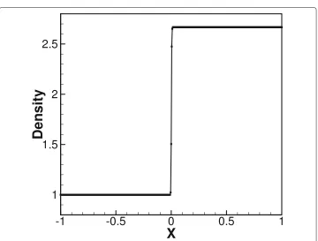
The initial state is the exact solution of the one-dimensional steady Euler equations. It should keep the same shape fort ≥ 0 when we run the code. However, because of the usage of the Lax-Friedrichs flux splitting, the initial condition isnota steady numeri-cal solution of the WENO scheme. The shock wave is smeared across a few grid points. Figure1is the numerical density distribution along the computational domain. The code is run to the non-dimensional time t = 120. We can see that the numerical result is essentially non-oscillatory: no noticeable oscillations can be observed. The profile of the numerical shock wave is quite sharp and appears monotone to the eye. From an engi-neering point of view, this result is quite satisfactory. Figure2contains the zoomed view (left) of the density distribution at the downstream of the shock wave and the time evo-lution (right) of the density at the pointx=0.01. We can see clearly that there are slight spurious oscillations downstream of the shock wave. The amplitude of the spurious oscil-lations is at the level around 10−3_{, which is about the size of the local truncation error}

of the scheme. This is the well known post-shock oscillation that appears downstream of slowly moving or steady numerical shocks. It is the culprit for the failure of high-order shock capturing schemes to converge to ideal steady states.

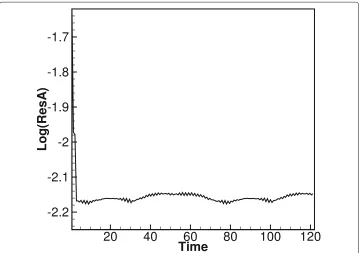
Figure3contains the time evolution of the average residue, which is defined as:

ResA=

n

i=1

|Ri|

N , (36)

whereRiis the local residue defined as

Ri= ∂ρ_∂

t

i

= ρin+1−ρin

t , (37)

andNis the total number of grid points.

Fig. 1Density distribution along the computational domain of 1D steady shock wave with Mach number

Fig. 2Zoomed density distribution (left) downstream of the shock wave and the time evolution of density at the pointx=0.01 (right) of the 1D steady shock wave with Mach numberM_∞=2.

We can see that the convergence property is not so satisfactory. Instead of converging to machine zero or to a small enough value, the average residue hangs around 10−2.2_.

Even though the flow variables do not change much in the long time running, the non-decreasing of the average residue after it reaches around 10−2.2 is a concern. This is because one can no longer use the size of the average residue to determine when to stop the computation, and must rely on experience including a visual comparison of the flow variables after many time steps to make this determination. Moreover, if we use this scheme to compute shock associated noises, the slight post-shock oscillation may be much stronger than the shock associated noises. Hence, it will influence the accuracy of the computation for the shock associated noises.

3.2 Two-dimensional isentropic vortex

The second example is a two-dimensional isentropic vortex, which is a smooth exact solution of two-dimensional steady Euler equations. We use this example to reveal the

convergence of WENO scheme to steady smooth flows. The parameters of the vortex is the same as that in [27,28]:

tangential velocity:uθ(r)=Mυre(1−r2)/2, radial velocity:ur=0,

pressure:p(r)= _γ1[ 1− γ−₂1M2_υe1−r2]γγ−1_,

density:ρ(r)=[ 1− γ−₂1M2_υe1−r2]γ1−1_{, wherer}=(_x−_x

v)2+(y−yv)2.

The center of the vortex is(xv,yv) =(0, 0). The strength of the vortex is set to beMυ =

0.25. The values at the ghost points in our computation are fixed as the exact solution. The computational domain is−4≤x≤4 and−4≤y≤4. A 400×400 equally spaced grid is used and the code is run to non-dimensional timet=50.

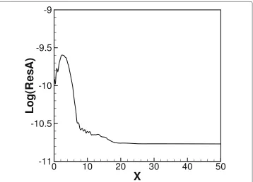
Figure4is the time evolution of the average residue. It converges to about 10−11, which is close to machine zero and is clearly small enough for us to use it as a criterion to stop the run. Figure5contains the density contours (dashed lines) and streamlines (solid lines with arrows). It can be seen that the streamlines and density contours are very smooth near the boundary.

The above two examples suggest that the reason for the non-convergence of the WENO scheme to steady state solutions of Euler equations is the slight post-shock oscillation. If we can find a technique to remove or reduce this post-shock oscillation, we could improve the convergence to steady states.

4 Strategies to improve the convergence to steady state solution for WENO schemes

4.1 A new smoothness indicator for the fifth-order WENO scheme

In [15], Zhang and Shu studied the relationship between the smoothness indicator and the appearance of the post-shock oscillation for the fifth-order WENO scheme. It was

Fig. 5Reproduced from [15]. The density contours (dashed lines from 0.9 to 1.0 with 30 levels) and streamlines (solid lines with arrows) of a two-dimensional isentropic vortex

found that the choice of the smoothness indicator is one reason to influence the appear-ance of the post-shock oscillations of the WENO schemes. Based on the physical analysis of the simple solution of the numerical shock and the characteristics of the different parts of the smoothness indicator, a new smoothness indicator was proposed for the fifth-order WENO scheme. With the new smoothness indicator, the slight post-shock oscillation of the fifth-order WENO scheme can be removed for some typical cases or reduced signif-icantly for some other cases. Therefore, the convergence property to steady state can be improved significantly.

To be more specific, the smoothness indicators given by (19) can be expanded as:

IS0= 1₄

2fx− 2₃fx32+₁₂13fx22+Ox6,

IS1= 1₄

2fx+ 2₃fx32+₁₂13fx22+Ox6,

IS2= 1₄

2fx− 2₃fx32+₁₂13fx22+Ox6.

(38)

Each of these formulae contains two parts P1 and P2. The first term P1 = 1

4

2fx± 2₃fx32includes the contribution from the first and third derivatives. The dominating contribution is from the first derivative. The second term is the second derivativeP2 = 13₁₂

fx22_{. The patterns ofP}

1andP2are quite different in the

indicator, it is a good choice to indicate the (lack of ) smoothness here. However, the sec-ond derivative takes a zigzag pattern in the neighborhood region of the shock wave. The absolute value of the second derivative takes its local maxima at both sides from the cen-ter of the numerical shock wave. At the cencen-ter of the shock wave, the absolute value of the second derivative takes its minimum. Based on the concept of the introduction of the smoothness indicator, the second derivative is not a good choice in the neighborhood region of the shock wave to indicate the (lack of ) smoothness here.

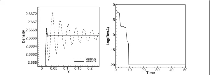
Based on this heuristic analysis, a new smoothness indicator for the fifth-order WENO scheme was proposed by just removing the contribution of the second derivatives in (19). It has the following form:

IS0=

fj−2−4fj−1+3fj

2

,

IS1=

fj−1−fj+1

2

,

IS2=

3fj−4fj+1+fj+2

2

.

(39)

With this technique, the same one-dimensional shock wave as in (35) is computed. The numerical solution is plotted in Fig.6, which contains the zoomed density distribution near the shock region and the time evolution of the residue. We can observe that the post-shock oscillation is removed and the residue can settle down to machine zero.

4.2 Upwind-biased interpolation

The new smoothness indicator proposed in [15] is only suitable for the fifth-order WENO scheme. It can not be applied to higher order WENO schemes. Moreover, even for the fifth-order WENO scheme, it may lead to the degeneration of the order of accuracy at some smooth extrema.

In [14], Zhang et al. studied the convergence property for higher order WENO schemes. They found that the post-shock oscillation is much stronger in the higher order WENO schemes and the non-convergence problem is more serious than that of the fifth-order WENO scheme. Through numerical tests, they found that the Roe averaging method in the local characteristic projection is a key reason to the appearance of the post-shock oscillation. Hence, they proposed an upwind-biased interpolation instead of the Roe averaging method in the local characteristic decomposition procedure. That is, (31) is replaced by:

U_i+1

2 =

U(1)_{, if u}

i+1₂ ≥0,

U(2), if u_i+1

2 <0.

(40)

Here,udenotes the velocity in the Euler equations. U(1) andU(2) are the interpolated values on the cell interface, which are computed either by the first-order, the second-order one-sided interpolation or the higher order upwind-biased WENO interpolation.

The first-order one-sided interpolation is:

U(1)=Ui, U(2)=Ui+1. (41)

The second-order one-sided interpolation is:

U(1)=(3Ui−Ui−1)/2, U(2)=(3Ui+1−Ui+2)/2. (42)

The procedure of the WENO interpolation is very similar to the WENO reconstruction. They use the same stencil and sub-stencils. In the large stencil, a higher order interpola-tion formula can be obtained; and in the sub-stencils, several lower order interpolainterpola-tions can be obtained. Using a similar convex combination, the WENO interpolation with the same order of accuracy as that on the large stencil can be obtained. In the following, only WENO interpolation procedure forU(1)based on the left-biased stencil is presented. The formulae to interpolateU(2)based on the right-biased stencil are symmetric with respect tox_i+1

2 and will not be shown. The detailed formulae forU

(1)_{are as follows.}

ˆ

U_iWENOI₊1

2 =

r−1

k=0

ωkUˆ_i(₊k)1 2

, (43)

whereUˆ(k)

i+1 2

is the lower order interpolation on each sub-stencil given by

ˆ

U(k)

i+1₂ = r−1

j=0

ckjUi−k+j (44)

with constant coefficientsckj. In the following, the fifth-order and seventh-order

interpo-lations are listed.

a. Fifth-order WENO interpolation

In the case ofr=3, the linear fifth-order interpolation is given by

U_i+1

2 =

1

128(3Ui−2−20Ui−1+90Ui+60Ui+1−5Ui+2). (45) The three third-order interpolations from the three sub-stencils are

U0

i+1

2 =

1

8(3Ui−2−10Ui−1+15Ui),

U1

i+1

2 =

1

8(−Ui−1+6Ui+3Ui+1),

U2

i+1₂ = 1

8(3Ui+6Ui+1−Ui+2).

(46)

The linear weights are given by

c0=

1

16, c1= 10

16, c2= 5

16, (47)

and the formulae of the smoothness indicators for the fifth-order WENO interpolation are the same as those of the fifth-order WENO reconstruction given by (19).

In the case ofr=4, the linear seventh-order interpolation is given by

U_i+1

2 =

1

1024(−5Ui−3+42Ui−2−175Ui−1+700Ui+525Ui+1−70Ui+2+7Ui+3). (48) The four fourth-order interpolations from the four sub-stencils are

U0

i+1

2 =

1

48(−15Ui−3+63Ui−2−105Ui−1+105Ui),

U1

i+1₂ = 1

48(3Ui−2−15Ui−1+45Ui+15Ui+1),

U2

i+1₂ = 1

48(−3Ui−1+27Ui+27Ui+1−3Ui+2),

U3

i+1

2 =

1

48(15Ui+45Ui+1−15Ui+2+3Ui+3).

(49)

The linear weights are

c0=

1

64, c1= 21

64, c2= 35

64, c3= 7

64, (50)

and the smoothness indicators are

IS0= Ui−3(79788Ui−3−566568Ui−2+680328Ui−1−273336Ui)

+Ui−2(1027692Ui−2−2523384Ui−1+1034568Ui)

+Ui−1(1610892Ui−1−1378728Ui)+308748U_i2,

IS1= Ui−2(38028Ui−2−232488Ui−1+228168Ui−71736Ui+1)

+Ui−1(401292Ui−1−847224Ui+277128Ui+1)

+Ui(492012Ui−364968Ui+1)+79788Ui2+1,

IS2= Ui−1(79788Ui−1−364968Ui+277128Ui+1−71736Ui+2)

+Ui(492012Ui−847224Ui+1+228168Ui+2)

+Ui+1(401292Ui+1−232488Ui+2)+38028U_i2₊₂,

IS3= Ui(308748Ui−1378728Ui+1+1034568Ui+2−273336Ui+3)

+Ui+1(1610892Ui+1−2523384Ui+2+680328Ui+3)

+Ui+2(1027692Ui+2−566568Ui+3)+79788Ui2+3.

(51)

This new local characteristic decomposition procedure can be applied to different vari-ants of WENO schemes, such as the one using the smoothness indicator proposed in [15], the one using the mapped technique proposed in [23], and the improved WENO scheme in [29].

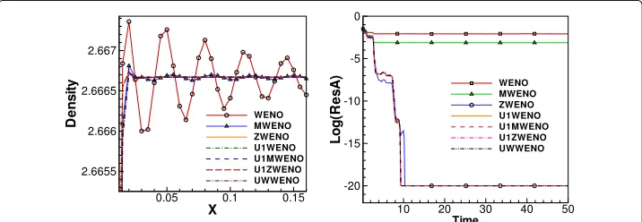
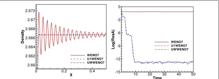
With this technique, the same problem of the one-dimensional steady shock wave of Mach number 2 is computed. Figures 7 and 8 contain the numerical results for the fifth-order WENO scheme and the seventh-order WENO scheme, respectively.

Fig. 8Reproduced from [13]. Numerical solution of the 1D steady shock wave with Mach numberM_∞=2 using the seventh-order WENO scheme with the upwind-biased interpolation. Left: zoomed density distribution downstream of the shock wave. Right: the time evolution of the average residue

From these numerical tests, we can conclude: (1) Upwind-biased interpolation is suit-able for all WENO schemes, including the traditional WENO scheme [6] (represented by WENO here), mapped WENO scheme [23] (MWENO), the improved WENO scheme by Don and Borges in [30] (ZWENO), and WENO schemes with general orders of accuracy. (2) For the fifth-order WENO scheme, the post-shock oscillation is reduced significantly and the residue can settle down to machine zero. (3) The post-shock oscillation is much stronger in higher order WENO schemes than those of fifth-order WENO scheme. With the upwind-biased interpolation, the post-shock oscil-lation is reduced significantly and the residue can go to a very small value close to machine zero.

Unfortunately, these strategies are not good enough for more complicated engineer-ing problems. In [14,15], several two-dimensional complex problems were tested for the WENO schemes with these strategies. The problems contain 135◦oblique shock wave, regular shock reflection on a wall, a supersonic flow past a forward step, and a supersonic flow past a plate. Except for the 135◦oblique shock wave case, the convergence for the other problems is not ideal, even though there are significant improvements compared with the traditional WENO schemes. The tests show that the convergence is sensitive to whether the numerical meshes are aligned with the shock wave. For the case of the 135◦oblique shock wave, the initial shock wave is located exactly on the grid points with

5 Application of the techniques to improve the convergence property to other types of weighted schemes

5.1 Fast sweeping WENO schemes

The fast sweeping method is a typical method to increase the convergence rate towards steady states. The main idea of the fast sweeping method is to combine the finite difference scheme and Gauss-Seidel iterations with alternating sweeping directions.

In [31–36], fast sweeping methods were developed for Eikonal equations and Hamilton-Jacobi equations. Combining the technique of the fast sweeping method and the strategies to improve the convergence to steady state solutions for WENO schemes [13,15], Wu et al. [37] developed a high-order fixed-point sweeping WENO method for steady state Euler equations. Different from other fast sweeping methods, the fixed-point iterative sweeping method has the advantages that they have explicit forms and do not involve inverse operation of nonlinear local systems. Numerical experiments show that the convergence to steady state solutions is much faster than the regular time-marching approach.

For the two-dimensional time dependent Euler Eq. (2), the semi-discretized equation is

∂U

∂t +

ˆ

Fi+1/2,j− ˆFi−1/2,j

x +

ˆ

Gi,j+1/2− ˆGi,j−1/2

y =0, i=1,· · ·,N; j=1,· · ·,M.

(52)

A Jacobi type Euler forward fixed-point iterative scheme is as the following:

U_ijn+1=U_ijn+ _α CFL

x/x+αy/yL

U_in_−r,j,· · ·,U_in_+s,j;U_ijn;U_in_,j−r,· · ·,U_in_,j+s

;

i=1,· · ·,N;j=1,· · ·,M. (53) Here,Lrepresents the difference operator of the WENO scheme. The corresponding fast sweeping scheme can be written as:

U_ijn+1=U_ijn+ _α CFL

x/x+αy/yL

U_i∗_−r,j,· · ·,U_i∗_+s,j;U_ijn;U_i∗_,j−r,· · ·,U_i∗_,j+s

;

i=1,· · ·,N;j=1,· · ·,M, (54) where the Gauss-Seidel philosophy is used here, which means that the newest value of

U, denoted byU∗, is used in the iteration.U∗could either beU_kn_,lorU_kn_,+_l1depending on the current sweeping direction. The iterations do not just proceed in only one direction

i = 1 : N,j = 1 : Mas in the time-marching approach (53), but in the following four alternating directions repeatedly, (1)i = 1 : N,j = 1 : M; (2)i = N : 1,j = 1 : M; (3)i=N: 1,j=M: 1; (4)i=1 :N,j=M: 1.

For the third-order TVD Runge-Kutta scheme,

U_ij(1)=U_ijn+tnL

U_in_−r,j,· · ·,U_in_+s,j;U_ijn;U_in_,j−r,· · ·,U_in_,j+s

,

U_ij(2)= 3₄U_ijn+ ₄1U_ij(1)+1₄tnL

U_i(₋1)_r,j,· · ·,U_i(₊1)_s,j;U_ij(1);U_i(_,1_j−)_r,· · ·,U_i(_,1_j+)_s,

U_ijn+1= 1₃Un

ij +23U

(2)

ij + 23tnL

U_i(₋2)_r,j,· · ·,U_i(₊2)_s,j;U_ij(2);U_i(_,2_j−)_r,· · ·,U_i(_,2_j+)_s,

i=1,· · ·,N;j=1,· · ·,M,

the RK type fixed-point sweeping scheme has the form

U_ij(1)=U_ijn+ _α CFL

x/x+αy/yL

U_i∗_−r,j,· · ·,U_i∗_+s,j;U_ij∗;U_i∗_,j−r,· · ·,U_i∗_,j+s

,

U_ij(2)=U_ij(1)+_4(α CFL

x/x+αy/y)L

U_i∗∗_−r,j,· · ·,U_i∗∗_+s,j;U_ij(1);U_i∗∗_,j−r,· · ·,U_i∗∗_,j+s

,

U_ijn+1=U_ij(2)+ _3(α 2CFL

x/x+αy/y)L

U_i∗∗∗_−r,j,· · ·,U_i∗∗∗_+s,j;U_ij(2);U_i∗∗∗_,j−r,· · ·,U_i∗∗∗_,j+s,

i=i1,· · ·,iN;j=j1,· · ·,jM.

(56)

In the three stage iterations of (56), the newest value is also used in the current sweeping directions, which are represented byU∗,U∗∗, andU∗∗∗respectively in each stage.

The feature of the numerical solution in the neighborhood region of the shock waves and the convergence property for the flow with shock waves in the fast sweeping WENO method are similar with those of WENO schemes. The use of the strategies to improve the convergence property of WENO schemes can also reduce the post-shock oscillation and improve the convergence ability. The fast sweeping technique can relax the stability condition and allow a larger CFL number, therefore leading to an increased convergence rate and decreased CPU time. The one-dimensional steady shock wave of Mach number 2 was computed in [37]. The amplitude of the post-shock oscillation, convergence prop-erty, the CPU costs, and the largest permitted CFL number were compared for different methods. Figure9contains the time evolution of the residues of different iterative meth-ods. The spatial discretization is the fifth-order WENO scheme with the new smoothness indicator. We can observe that the largest CFL number of the Euler forward method is only 0.3. When the fast sweeping is used, a much larger CFL number, 1.1, is permitted. The CPU cost is saved. More details can be found in [37].

5.2 Weighted compact schemes

Linear compact schemes [38] are a typical type of high-order numerical schemes. They have the feature of high-order, low dissipation, and have been applied in many areas. However, linear compact schemes can not simulate flows containing strong shock waves. Combining linear compact schemes and WENO schemes, a series of weighted compact schemes were developed in [14,39,40]. The weighted compact scheme was developed based on the cell-centered compact scheme proposed by Lele [38],

βf_i−2+αf_i−1+f_i+αf_i+1+βf_i+2=c

f_i+5

2 −fi−52

5x +b

f_i+3

2 −fi−32

3x +a

f_i+1

2 −fi−12

x . (57)

The left hand side of the linear compact scheme (57) is a linear combination of the spatial derivativesf_iat some grid nodes and the right hand side is a linear combination of some cell-centered valuesf_i+1

2. Ifβ = 0,c= 0, a fourth order tridiagonal compact scheme is

obtained with:a= 3₈(3−2α),b= 1₈(22α−1). The corresponding scheme is:

αf_i−1+f_i+αf_i+1=b

f_i+3

2 −fi−32

3x +a

f_i+1

2 −fi−12

x . (58)

Ifα= ₆₂9, we obtain a sixth-order tridiagonal scheme. Especially, ifα= ₂₂1, the coefficient

bvanishes. It results in the most compact scheme as follows:

αf_i−1+f_i+αf_i+1=a

f_i+1

2 −fi−12

x . (59)

In (57), (58) and (59), the right hand side cell-centered values are unknowns. In [38], Lele proposed a compact formula to interpolate the unknown values on cell-centers from the values of neighboring grids. The obtained compact scheme is linear. Instead of using compact interpolation, Deng and Zhang [39] and Zhang et al. [14,40] used WENO inter-polation to compute the cell-centered values. The obtained schemes are the weighted compact schemes. The detailed formulae for the WENO interpolation are given by (43) and (44) in Section4.2.

In [12,14], Zhang et al. studied the convergence property to steady state solutions of Euler equations for weighted compact schemes. It is shown that the weighted compact schemes suffer from the same problem as WENO schemes. There is still slight post-shock oscillations, preventing the residue from settling down to a satisfactory small value. Because the WENO interpolation is quite similar with the WENO reconstruction, the strategies to improve the convergence to steady state solution for the WENO schemes are applicable also to weighted compact schemes. The same one-dimensional steady shock wave was computed in [12,14] to test the behavior of the numerical solution, the post-shock oscillation, and the convergence feature of the weighted compact scheme with the strategies to improve the convergence property of WENO schemes. Similar conclusions were obtained. The post-shock oscillation is reduced significantly and the residue can go to a small value close to machine zero. The details can be found in [12,14].

6 A new type of WENO schemes

6.1 The new WENO schemes

schemes [16,17,19]. Thus we have the associated semidiscretization of (6) and reformu-late it as (33). Since the fifth-order version is taken as an example in this paper, we require

1

x

ˆ

fi+1/2− ˆfi−1/2

to be a fifth-order approximation tof(u)x. For upwinding and

sta-bility, we also split the fluxf(u)intof(u) = f+(u)+f−(u)and then approximate each of them separately using its own wind direction. The simple Lax-Friedrichs flux split-ting is used again. All the one-dimensional and two-dimensional finite difference WENO schemes are based on the simple reconstruction procedure detailed below. Suppose we are given the cell averagesw¯j= 1_x

xj+1/2

xj−1/2 w(x)dxfor alljand would like to obtain a

fifth-order WENO polynomial approximationwi(x)defined onIi =[xi−1/2,xi+1/2], based on

an upwind-biased stencil consisting ofIj=[xj−1/2,xj+1/2] withj=i−2, ...,i+2. The

pro-cedure in [16,17], with similar ideas in earlier references [41–43] as well, is summarized as follows.

Step 2.1:We choose the following big spatial stencilS1= {Ii−2, ...,Ii+2}and reconstruct

a quartic polynomialf1(x)satisfying

1

x

xj+1/2

xj−1/2

f1(x)dx= ¯wj, j=i−2, ...,i+2. (60)

We also choose two smaller spatial stencils S2 = {Ii−1,Ii} and S3 = {Ii,Ii+1}, and

reconstruct two linear polynomials satisfying

1

x

xj+1/2

xj−1/2

f2(x)dx= ¯wj, j=i−1,i, (61)

and 1

x

xj+1/2

xj−1/2

f3(x)dx= ¯wj, j=i,i+1. (62)

Step 2.2:We rewrite the quartic polynomialf1(x)as:

f1(x)=γ1

1

γ1

f1(x)−

3

=2

γ γ1

f(x)

+

3

=2

γf(x). (63)

Clearly, (63) holds true for arbitrarily positive linear weightsγ on the condition that ₃

=1γ=1.

Step 2.3:We compute the smoothness indicatorsISk,k = 1, 2, 3, which measure how

smooth the functionsfk(x), k = 1, 2, 3, are in the interval [xi−1/2,xi+1/2], by using the

classical recipe for the smoothness indicators (16).

Step 2.4:We calculate the nonlinear weights, by adopting the strategy in WENO-Z as specified in [29,30,44]

τ =

|IS1−IS2| + |IS1−IS3|

2

2

, (64)

and

ωn= ₃ω¯n =1ω¯

, ω¯n=γn

1+ τ

ε+ISn

, n=1, 2, 3. (65)

Hereεis defined as a tiny positive number as before.

Step 2.5:We replace the linear weights in (63) with the nonlinear weights (65), and the final reconstruction polynomialwi(x)is given by

wi(x)=ω1

1

γ1

f1(x)−

3

=2

γ γ1

f(x)

+

3

=2

The construction of the numerical fluxfˆ_i−_+1/2is mirror-symmetric with respect toxi+1/2.

Finally, the semidiscrete scheme (3) is discretized in time by (34).

Let us mention a few features and advantages of the new WENO schemes. The first is that the linear weights can be any positive numbers on the condition that their sum is one. The second is their simplicity and easy extension to multi-dimensions. The third is that three unequal-sized central/biased spatial stencils are used in the WENO spatial reconstructions. The fourth is such new WENO schemes could main-tain fifth-order accuracy in smooth regions and degrade to second-order accuracy in non-smooth regions, which are different from the fifth-order classical WENO schemes [6] (whose degenerated order is three). The last is that the number of spatial stencils is no bigger than that of the same fifth-order classical finite difference or finite vol-ume WENO schemes [6]. We refer to [16–18, 20, 22] for more details on these new finite difference and finite volume WENO schemes on structured and unstructured meshes.

6.2 The convergence to steady state solution of the new WENO schemes

This new type of WENO schemes uses a convex combination of a quartic polynomial with two linear polynomials on unequal-sized spatial stencils in one dimension and two dimensions. Such new finite difference WENO schemes use the same information as the classical WENO scheme [6] and yield the same fifth-order in smooth regions, yet they have a few advantages over the classical WENO scheme [6], one of them being that the new WENO schemes can provide a unified polynomial approximation in the whole cell with the same nonlinear weights, comparing with the classical WENO scheme which involves different linear and nonlinear weights for different points on the cell boundaries. Computational results in [16,17] indicate that this new type of WENO schemes works well for time-dependent test problems, but this is not what we would like to focus on in this paper.

6.3 Shock reflection problem

In this section, we perform one typical example to test the steady state computation per-formance of the new fifth-order finite difference WENO scheme [16,19] and term it as ZQSWENO scheme. We also make a comparison with the fifth-order classical finite dif-ference WENO scheme [6] and term it as JSWENO scheme. The CFL number is 0.6. The average residue is defined as

ResA=

N

i=1

|R1i| + |R2i| + |R3i| + |R4i|

4×N , (67)

whereR∗i are local residuals of different conservative variables, that is,R1i = ∂ρ_∂t|i = ρn+1

i −ρin

t , R2i = ∂(ρ u) ∂t |i =

(ρu)ni+1−(ρu)ni

t ,R3i = ∂(ρ v) ∂t |i =

(ρv)ni+1−(ρv)ni

t , R4i = ∂∂Et|i = En_i+1−En

i

t , andNis the total number of grid points. Notice that here we are using a single

indexito list all the two-dimensional grid points. The linear weights are set asγ1=0.98

andγ2=γ3=0.01 in this section.

The computational domain is a rectangle of length 4 and height 1. The boundary con-ditions are that of a reflection condition along the bottom boundary, supersonic outflow along the right boundary and Dirichlet conditions on the other two sides:

(ρ,u,v,p)T=

(1.0, 2.9, 0, 1.0/1.4)T|_(0,y,t)T,

(1.69997, 2.61934,−0.50632, 1.52819)T_| (x,1,t)T.

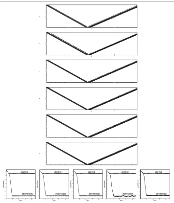
Initially, we set the solution in the entire domain to be that at the left boundary. We show the density contours with 15 equally spaced contour lines from 1.10 to 2.58 in Fig.10, after numerical steady state is reached. The history of the residue (67) as a function of time is also shown in Fig.10. The difference between the two types of WENO schemes can be clearly observed from the residue history. It can be observed that the average residue of the JSWENO scheme can only settle down to a value around 10−1, while the average residue of the ZQSWENO scheme withε= 10−2_{,ε= 10}−4_{,ε = 10}−6_{,ε = 10}−8_{, and}

ε=10−10_{can settle down to a value around 10}−12.5_{, close to machine zero.}

7 Conclusion

The convergence to steady state solutions is a key problem for shock capturing schemes. It becomes more difficult for high-order shock capturing WENO schemes. The key reason is there is a slight post-shock oscillation.

Two techniques have been developed to improve the convergence to steady state solu-tions of Euler equasolu-tions for high-order WENO schemes. One is a new smoothness indicator, which was proposed for the fifth-order WENO scheme. The other is an upwind-biased interpolation, introduced to compute the physical value at the cell interface in the procedure of the local characteristic projection replacing the traditional Roe average for general WENO schemes. With these techniques, the slight post shock oscillation can be removed or reduced significantly. The convergence property to steady state solution is improved. Moreover, these two techniques are applicable to other weighted schemes such as the fast sweeping WENO schemes and weighted compact schemes.

X

Y

0 1 2 3 4

0 0.5 1

X

Y

0 1 2 3 4

0 0.5 1

X

Y

0 1 2 3 4

0 0.5 1

X

Y

0 1 2 3 4

0 0.5 1

X

Y

0 1 2 3 4

0 0.5 1

X

Y

0 1 2 3 4

0 0.5 1 Time Log1 0 (R e s A )

5 10 15 20 -14 -12 -10 -8 -6 -4 -2 0 JSWENO ZQSWENO(1) Time Log1 0 (R e s A )

5 10 15 20 -14 -12 -10 -8 -6 -4 -2 0 JSWENO ZQSWENO(2) Time Log1 0 (R e s A )

5 10 15 20 -14 -12 -10 -8 -6 -4 -2 0 JSWENO ZQSWENO(3) Time Log1 0 (R e s A )

5 10 15 20 -14 -12 -10 -8 -6 -4 -2 0 JSWENO ZQSWENO(4) Time Log1 0 (R e s A )

5 10 15 20 -14 -12 -10 -8 -6 -4 -2 0 JSWENO ZQSWENO(5)

Fig. 10 The shock reflection problem. From top to bottom and left to right: 15 equally spaced density contours from 1.10 to 2.58 of JSWENO scheme; ZQSWENO scheme with (1)ε=10−2, (2)ε=10−4, (3)

ε=10−6, (4)ε=10−8, and (5)ε=10−10; the evolution of the average residue. 121×31 points

The residue can reach a tiny value close to machine zero for a large class of test prob-lems, including the difficult two-dimensional problems where the shocks pass through the boundary of the computational domain.

In the viewpoint of applications, the convergence to steady state solution of high-order WENO schemes is still a difficult problem for complex engineering problems. However, with the advance made over the past years, as reviewed in this paper, especially the new type of WENO schemes summarized in Section6, we have a good hope to overcome this difficulty of convergence to steady state solutions for complex engineering problems.

Acknowledgements No.

Authors’ contributions

Authors’ information

The information of all authors are included in the first page of this paper.

Funding

The work of the first author was supported by NSFC grant 11732016. The research of the second author was supported by NSFC grant 11872210. The research of the third author was supported by NSF grant DMS-1719410.

Availability of data and materials

All data and materials are available from the authors of this paper.

Competing interests

The authors declare that they have no competing interests.

Author details

1_{State Key Laboratory of Aerodynamics, China Aerodynamics Research and Development Center, Mianyang, Sichuan}

621000, China.2_{College of Science, Nanjing University of Aeronautics and Astronautics, Nanjing, Jiangsu 210016,}

People’s Republic of China.3_{Division of Applied Mathematics, Brown University, Providence, RI 02912, USA.}

Received: 29 April 2019 Accepted: 17 June 2019

References

1. Harten A (1983) High resolution schemes for hyperbolic conservation laws. J Comput Phys 49:357–393 2. Harten A, Engquist B, Osher S, Chakravarthy S (1987) Uniformly high order essentially non-oscillatory schemes, III. J

Comput Phys 71:231–303

3. Shu C-W, Osher S (1988) Efficient implementation of essentially non-oscillatory shock capturing schemes. J Comput Phys 77:439–471

4. Shu C-W, Osher S (1989) Efficient implementation of essentially non- oscillatory shock capturing schemes II. J Comput Phys 83:32–78

5. Balsara DS, Shu C-W (2000) Monotonicity preserving weighted essentially non-oscillatory schemes with increasingly high order of accuracy. J Comput Phys 160:405–452

6. Jiang G-S, Shu C-W (1996) Efficient implementation of weighted ENO schemes. J Comput Phys 126:202–228 7. Liu XD, Osher S, Chan T (1994) Weighted essentially non-oscillatory schemes. J Comput Phys 115:200–212 8. Zhang HX (1984) The exploration of the spatial oscillations in finite difference solutions for Navier-Stokes shocks.

ACTA Aerodyn Sin 1(1):12–19. (in Chinese)

9. Zhang HX (1988) Non-oscillatory and non-free-parameter dissipation difference scheme. ACTA Aerodyn Sin 6(2):143–165. (in Chinese)

10. Zhang HX, Zhuang FG (1991) NND schemes and their applications to numerical simulation of two and three dimensional flow. Adv Appl Mech 29:193–256

11. Osher S, Chakravarthy C (1984) High resolution schemes and the entropy condition. SIAM J Numer Anal 21:955–984 12. Zhang S, Deng X, Mao M, Shu C-W (2013) Improvement of convergence to steady state solutions of Euler equations

with weighted compact nonlinear schemes. Acta Math Applicatae Sin Engl Ser 29:449–464

13. Zhang S, Jiang S, Shu C-W (2011) Improvement of convergence to steady state solutions of Euler equations with the WENO schemes. J Sci Comput 47:216–238

14. Zhang S, Jiang S, Shu C-W (2008) Development of nonlinear weighted compact schemes with increasingly higher order accuracy. J Comput Phys 227:7294–7321

15. Zhang S, Shu C-W (2007) A new smoothness indicator for the WENO schemes and its effect on the convergence to steady state solution. J Sci Comput 31:273–305

16. Zhu J, Qiu J (2016) A new fifth order finite difference WENO scheme for solving hyperbolic conservation laws. J Comput Phys 318:110–121

17. Zhu J, Qiu J (2017) A new type of finite volume WENO schemes for hyperbolic conservation laws. J Sci Comput 73:1338–1359

18. Zhu J, Qiu J (2017) A new third order finite volume weighted essentially non-oscillatory scheme on tetrahedral meshes. J Comput Phys 349:220–232

19. Zhu J, Shu C-W (2017) Numerical study on the convergence to steady state solutions of a new class of high order WENO schemes. J Comput Phys 349:80–96

20. Zhu J, Shu C-W (2018) A new type of multi-resolution WENO schemes with increasingly higher order of accuracy. J Comput Phys 375:659–683

21. Zhu J, Shu C-W (2019) Numerical study on the convergence to steady state solutions of a new class of finite volume WENO schemes: Triangular meshes. Shock Waves 29:3–25

22. Zhu J, Shu C-W (2019) A new type of multi-resolution WENO schemes with increasingly higher order of accuracy on triangular meshes. J Comput Phys 392:19–33

23. Henrick AK, Aslam TD, Powers JM (2005) Mapped weighted essentially non-oscillatory schemes: achieving optimal order near critical points. J Comput Phys 207:542–567

24. Roe PL (1981) Approximate Riemann solvers, parameter vectors, and difference schemes. J Comput Phys 43:357–372 25. Shu C-W (1988) Total-Variation-Diminishing time discretizations. SIAM J Sci Stat Comput 9:1073–1084

26. Saad MA (1993) Compressible Fluid Flow, Prentice Hall, Englewood Cliffs, NJ, USA