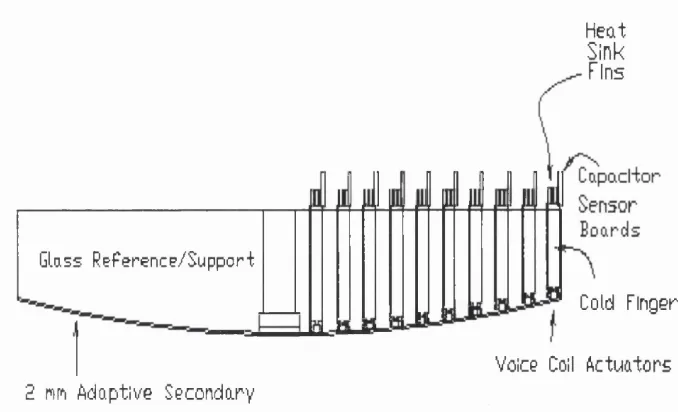
A deformable secondary demonstrator for adaptive optics

A D eform able Secondary D em on strator

for A d ap tive O ptics

A Thesis Submitted for the Degree

of

Doctor of Philosophy of the University of London

by

Jun Ho Lee

pzZ

---Optical Science Laboratory

Department of Physics and Astronomy

University College

University of London

ProQ uest Number: 10016152

All rights reserved

INFORMATION TO ALL U SE R S

The quality of this reproduction is d ep en d en t upon the quality of the copy subm itted. In the unlikely even t that the author did not sen d a com plete manuscript

and there are m issing p a g e s, th e se will be noted. Also, if material had to be rem oved, a note will indicate the deletion.

uest.

ProQ uest 10016152

Published by ProQ uest LLC(2016). Copyright of the Dissertation is held by the Author. All rights reserved.

This work is protected against unauthorized copying under Title 17, United S ta tes C ode. Microform Edition © ProQ uest LLC.

ProQ uest LLC

789 East E isenhow er Parkway P.O. Box 1346

A b str a c t

C on ten ts

A b stra ct 3

List o f F igures 9

L ist o f Tables 18

G lossary 20

1 In trod u ction 22

1.1 B a c k g ro u n d ... 22

1.2 Adaptive Secondary Mirror ... 24

1.3 The A uthor’s Contributions and Contents of the T h e s is ... 25

1.3.1 The A uthor’s C o n trib u tio n s ...26

1.3.2 Contents of the T h e s i s ... 27

2 W h a t is A d a p tiv e O ptics? 28 2.1 Adaptive Optics S y ste m s... 28

2.1.1 Guide S t a r s ...29

2.1.2 Wavefront Sensors ...30

2.1.3 Wavefront Correction D e v ic e s ... 33

2.1.4 Wavefront Control S y s te m ...36

2.2 Wavefront Distortion By the A tm o sp h ere... 38

2.2.1 Spatial Phase V a ria tio n s ... 38

2.2.2 Temporal Phase V ariatio n s...39

2.2.3 Atmospheric Turbulence and Zernike P o ly n o m ia ls...40

2.2.4 Angular Iso p lan atism ... 42

2.2.5 C^{h) Variation with H e ig h t...43

2.3 Scientific Drivers for Adaptive O p tic s ... 45

3 W h y A d a p tiv e Secondary M irrors? 46 3.1 Throughput, Emissivity, and Polarisation C om parison... 46

3.1.1 T h r o u g h p u t...48

3.1.2 E m issiv ity ... 50

3.1.3 P o la ris a tio n ...52

3.2 Location of an Adaptive Secondary Mirror as a Wavefront Corrector . 55 3.3 World-wide Development of Adaptive Secondary Mirror Systems . . . 59

3.4 Previous Deformable Secondary Mirror Work at the O S L '...61

4 D esig n in g th e dem on strator 63 4.1 Defining the Demonstrator P r o j e c t ... 63

4.2 W hat is the d em o n strato r?... 64

4.3 Requirements for the d e m o n s tr a to r ... 65

4.3.1 Mirror Substrate I n te g r i t y ...65

4.3.2 High System Reliability ... 66

4.3.3 Temporal Response Requirements and Required Stroke of Ac­ tuators ... 67

4.4 Mechanical D e s i g n ... 70

4.4.1 Mirror S u b s t r a t e ... 70

4.4.3 C u p s ...75

4.4.4 Flexure C o u p lin g ... 78

4.4.5 Actuators and Displacement S e n s o r s ... 78

4.4.6 Actuator M o u n ts ... 81

4.4.7 Support p l a t e ...82

4.5 Drive Electronics D e s ig n ... 83

4.5.1 Closed Loop Actuator C o n tro l...83

4.5.2 A c tu a to r ... 84

4.5.3 Strain Gauge and W heatstone B rid g e ...85

4.5.4 Pre-amplifier ...86

4.5.5 Error A m p lifie r... 87

4.5.6 Actuator Power A m p lif ie r ... 88

4.5.7 Simulation of the D e s ig n ... 89

4.5.8 Thermal D r i f t ...90

5 Perform ance P red iction s 92 5.1 In tro d u c tio n ...92

5.2 Finite Element A n a l y s i s ... 92

5.2.1 Finite Element Modelling ... 93

5.2.2 R e su lts...94

5.3 Performance P r e d ic tio n s ... 101

5.3.1 Fitting Error ...101

5.3.2 Defining the Best-fit Z j of the D e m o n stra to r... 103

5.3.3 R e su lts...104

5.4 Conclusion and D isc u ssio n ...108

6.1 A ctuator Tests ...I l l 6.1.1 Hysteresis and Linearity T e s t s ... I l l

6.1.2 Stability T e s t ... 112

6.1.3 Dynamic T e s t ... 115

6.1.4 Resolution T e s t ...119

6.2 Life Tests of the flexure coupling ...122

6.3 Production of the mirror substrate ...122

6.3.1 Machining and P re-polishing... 123

6.3.2 Pre-polishing T e s tin g ... 126

6.3.3 C o a t i n g ... 128

6.3.4 P olishing... 128

6.3.5 T e stin g ... 129

6.3.6 Discussion of the T e s tin g ...132

6.4 Assembly/Disassembly of the D e m o n s tr a to r ...133

6.4.1 The First Assembly T r ia l...133

6.4.2 The Second Trial Assembly ... 134

6.4.3 D isassem bly... 140

6.4.4 The Third Assembly T r i a l ...141

7 L aboratory T ests 144 7.1 A Controlled Switch-off P r o c e s s ... 144

7.2 Flexure Test of the M i r r o r ... 146

7.3 Control System Setup ... 149

7.4 Static E v a lu a tio n ... 150

7.4.1 Influence F u n c tio n s ...150

7.4.2 Lower order Zenike f l t t i n g ...152

8 C on clusions &: Future work 159

A ck n ow led gem en t 172

A A p u p il-im aging gradient sensor 174

A .l S im u latio n ... 175

A .1.1 Sensor O u tp u t... 175

A. 1.2 R e su lts... 178

A. 1.3 Effects of the edge of the s e n s o r ...178

A.2 T e stin g ...180

A.2.1 O v erlap p in g ...180

A.2.2 Overall tip /tilt s e n s in g ... 182

List o f Figures

1.1 Schematic diagram of an adaptive optics system. (Prom http:/www. aoinc.com/A O S/Aotutorial.html: reprinted with permission from Adap­ tive Optics Associates, Inc. a unit of Hamilton Standard, a UT co.

... 24

1.2 Schematic of the adaptive secondary mirror system in the 6.5 m Multi-Mirror Telescope (MMT) adaptive optics [81]... 25

2.1 Schematic illustration of the use of mesospheric sodium as an artificial star for adaptive optics, (from h ttp ://t4 .lanl.gov/pw m /adaptive.htm l: with permission from P. M ilo n n i) ...30 2.2 Focal-anisoplanatism error arises not only from the unsampled tu r­

bulence above the beacon altitude, but also from the portion of the turbulence below the beacon altitude th at is sampled incorrectly be­ cause of the difference between the ray paths of the radiation from the beacon and the star (reproduced from Zollars [8] ) ... 31 2.3 Schematic diagram of Hartmann-Shack wavefront sensor. (From http:

/ www.aoainc.com/AOS/ A otutorial.htm l: reprinted with permission from Adaptive Optics Associates, Inc. a unit of Hamilton Standard,

a UT CO. ( 1 9 9 7 ) )... 33

2.4 Cross section of a bimorph deformable m i r r o r ... 35 2.5 Infrared absorption by atmospheric gases, reproduced from S.L. Val­

ley [ 9 7 ] ... 38 2.6 Time averaged C^(h) profile given by Valley [44] with height h (km):

3.1 Bigelow’s results on total reflectivity for multiple reflections (1, 3, 5, 10, 15, and 20) [ 1 0 ] ... 47 3.2 a) Reflectivity (%) of overcoated silver coating [29] b) Reflectivity (%)

of broadband multi-layer anti-reflection coatings [2 9 ]... 49 3.3 Total throughput (%) for the MMT and W HT AO systems in poly­

chromatic wavefront sensing, a) For wavefront sensing (centred at 0.7 iim) b) For science instrument (centred at 2.2 fim). The solid and dotted lines represent the results of the author and Bigelow [10, 11], respectively... 50 3.4 Emissivity(%) for MMT and W HT AO systems for science instru­

ments (around 2.2 f i m )... 51 3.5 Polarisation reflectivity curves for perpendicular reflections Rj. and

parallel reflections Ry, for a) aluminum and b) silver. Note the dif­ ference in vertical scales...53 3.6 Schematic of the WHT AO system reproduced from Bigelow [10, 11] . 54 3.7 Final optical layout of the WHT AO system upto the science pickoff

(NAOMI) [ 8 5 ] ... 54 3.8 A schematic diagram of a) seeing conjugation and b) pupil conjugation 57 3.9 UKIRT pupil vignetting due to seeing conjugation, fractional loss, by

height and angle. Reproduced from Bigelow [10, 1 1 ] ...58 3.10 Pupil conjugation with shear and vignetting at the secondary mirror . 58 3.11 The fast adaptive tip /tilt and focus secondary mirror for UKIRT, re­

produced from http://w w w .m pia-hd.m pg.de/M PIA /Projects/U K IR T / with kind permission of Andreas Glindemann VLTI group, ESO, Ger­ man ... 60 3.12 Gross-sectional view of the adaptive secondary mirror developed at

the Genter for Astronomical Adaptive Optics (GAAG), University of Arizona, reproduced from http://athene.as.arinoa.edu:8000/caao

/adapt.sec.html with, kind permission of Michael Lloyd-Hart, Steward

4.1 The proposed design of 1 meter diameter ASM with 90 actuators for

the Gemini telescope [11]... 64

4.2 Drawing of a 1 m mirror with 90 actuators positioned at + marks in the drawing. Small offset circle represents the dem onstrator of 270 mm diameter with 7 actuators... 65

4.3 Optical layout of the demonstrator AO system on the optical bench in the GHRIL... 66

4.4 Histogram of seeing data from the Cassegrain autoguider and the DIMM. The DIMM values are normalised to the same peak value as the autoguider (regenerated from h ttp:://ingAac.es/nom /histo.htm l with permission of Neil O Mahony)... 68

4.5 Median seeing for each month from the WHT autoguiders and the DIMM from Jan 93 to Jan 97 (regenerated with from http:://ing. iac.es / n o m / seasonal.html with permission of Neil O M ahony)... 68

4.6 The preliminary design of the dem onstrator... 71

4.7 Mechanical drawing of the assembled dem onstrator... 71

4.8 Mechanical drawing of the faceplate (units in m m )...72

4.9 Schematic diagram of coupling between the faceplate and an actuator. 73 4.10 Mechanical drawing of the boss (units in m m )... 74

4.11 Mechanical drawing of the cup (units in m m )... 76

4.12 Schematic diagram of the assembly setup... 76

4.13 Mechanical drawing of the flexure (units in m m )...78

4.14 A picture of the cups, the bosses and the flexures... 79

4.15 Cross section of the MS actuator [31] (units in m m )... 80

4.16 A Picture of the MS actuator with the flexure... 80

4.17 Actuator clamps... 82

4.19 Closed loop control of the actuators with a strain gauge sensor. . . . 83

4.20 Circuit diagram for the drive electronics... 84

4.21 Schematic diagram for the strain gauge bridge... 85

4.22 Schematic diagram for the pre-amplifier... 87

4.23 Schematic diagram for the error amplifier...87

4.24 Schematic diagram for the actuator power amplifier...88

4.25 The modelling of the drive electronics in a commercial software package. 89 4.26 Simulated amplitude transfer function of the drive electronics against the frequency of input signal from the DAC... 90

5.1 The finite elements model of the dem onstrator... 93

5.2 Defiections of the mirror substrate of the demonstrator due to gravity under a) Zenith pointing and b) horizontal pointing. The magnitudes of the defiections are expressed by the different colours. The values which colours represent are also shown in this figure. Note the differ­ ent colour scales between two figures... 96

5.3 The first 4 resonant modes of the dem onstrator respectively at 1) 547.22 HZ, 2) 644.86 Hz, 3) 709.77 Hz and 4) 1778.2 Hz... 97

5.4 The infiuence functions of the central and outer actuator when each actuator is pushed by 1 fim respectively. The defiections are displayed by colours. The values which the colours represent are also in the figures. Note the different colour scales...98

5.5 FEA results of the ASM demonstrator, the deformation of the demon­ strator when the central and the outer actuator are pushed by 1 /im respectively... 99

5.6 FEA results of the ASM demonstrator, stresses of the central fiexure when the central actuator was pushed by 1 /zm... 100

5.8 An example of the approximation of a circular aperture of radius

R — 1 with 49 elements. The shadowed region in this figure shows

the area of the 18*^ element represents. S is the width of the square element ... 104 5.9 3D plots of FEA results, the influence functions... 105 5.10 Zernike terms Zj {Z2 through Z5) and the corresponding best fit terms

Z j by the dem onstrator ... 106 5.11 aij (eqn. 5.11) between the first 22 Zernike terms Zj and the best

fit terms Z j. This figure represents orthogonality between the Zernike terms Zi and the best-fit terms Z j. In this plot, a z-axis value of 1 means perfect matching while 0 means perfect orthogonality. 107 5.12 Diagonal terms of aij (eqn. 5.11 and figure 5.11) between the first 22

Zernike terms Zj and the best fit Z j. This plots shows how well the mirror matches the Zernike polynomials. A z-axis value of 1 means perfect matching while 0 means zero-ability to fit the term ... 107 5.13 Strehl Ratio of the demonstrator ...108 5.14 Two orthogonal modes of Bigelow’s 36 actuator model, which most

closely approximate the Zernike tip /tilt modes [10, 11]... 110

6.1 Results of actuator and strain gauge hysteresis and linearity... 112 6.2 Schematic diagram of the stability test s e t u p ... 113 6.3 Movement of the actuator for constant inputs (0, 0.3, 0.6, 0.9, 1.2

volts) referred to the initial zero position at zero voltage input . . . .1 1 3 6.4 The therm al output of the strain gauge [95]...114 6.5 Maximum thermal drift of the actuator after 30 minutes with constant

inputs. Dotted line is the quadratic best fit curve... 115 6.6 A picture of the unit of the control drive e le ctro n ic s... 116 6.7 Hysteresis curve for sinusoidal input signals of two amplitudes (1 ,4

6.8 Strain gauge output vs. input signal to the drive electronics. Fre­

quency = 1 Hz, 10 cycles 117

6.9 Amplitude transfer function of seven closed loop actuators at 0.3 volts am plitude...118 6.10 Amplitude transfer function of one actuator for different am plitude

(0.3, 0.65, 1.15, 1.5 volts) sinusoidal inputs... 119 6.11 The eddy current sensor output for zero movement... 120 6.12 The signal of the eddy current sensor and strain gauge bridge for

linearly increasing control signal (0.5m V /sec)...121 6.13 The signal of the eddy current sensor and strain gauge bridge signal

for linearly increasing control signal (O .lv/sec)...121 6.14 Schematic diagram of the flexure coupling life test setup... 123 6.15 The mechanical drawings of the mandrels... 124 6.16 The mirror blank was ground against the rear tool (figure 6.15-b). . . 125 6.17 A lap of pitch with 25 mm square facets prepared for the polishing

and the polished mirror substrate...126 6.18 The fringes of the mirror surface obtained by a scatter plate interfer­

ometer during the pre-polishing tests... 127 6.19 A picture of the polishing...128 6.20 Optical setup of the test tower...129 6.21 Schematic diagram of a scatter plate interferometer (Drawn by D.H.

Kim )... 130 6.22 One measurement of the faceplate with 9 fringes: a) Fringes and b)

OPD calculated from the fringes...130 6.23 One measurement of the faceplate with 14 fringes: a) Fringes and b)

OPD calculated from the fringes...131 6.24 The coordinate system by which the aberrations were specified and

6.25 One measurement of the faceplate three months after the first mea­ surements (figure 6.22, 6.23): a) Fringes and b) OPD calculated from

the fringes... 134

6.26 The picture of the demonstrator with fringes after the first trial as­ sembly...135

6.27 Positions of the actuators on the faceplate and numbering the actuators. 135 6.28 Interferograms of the mirror as the boss was threaded into the back surface of the mirror and was tightened... 136

6.29 Schematic front view of the vertical mounting of the mirror for optical testing...137

6.30 Interferograms before and after the seven bosses were screwed into the back plate of the mirror and were secured with a thread locking adhesive...138

6.31 Interferograms of the mirror after the second trial assembly... 139

6.32 The deformation of the backing plate during the assembly calculated using FEA ...140

6.33 Interferogram after disassembly...141

6.34 Interferogram after the third assembly tria l... 142

6.35 A picture of the demonstrator unit after assembly... 143

7.1 Four fringes of the switch on/off sequence measured using a He-Ne laser of 0.6328 //m wavelength: a) System switched off, b) System switched on but actuators at near zero random positions, c) After sinusoidal cycling of all actuators and d) After system switched off. . 145

7.2 A preliminary test to calibrate the assembled demonstrator. Displace­ ments of various points were measured while an actuator was being actuated with a sinusoidal input of 1 Volt and 0.02 Hz...147

7.3 A picture of the assembled dem onstrator and a schematic diagram of the deformation of the actuator m ount... 148

7.5 The DOS mirror control interface (written in Q-Basic)...150 7.6 Optical setup to measure the deformation of the dem onstrator...151 7.7 Measured influence functions of the central and outer actuators. The

influence functions have been rescaled to have a maximum of 1 /zm. . 151 7.8 The measured mirror deformation to match the first four Zernike

terms: Two tilts, defocus, astigm atism ...153 7.9 The measured residual errors of the mirror deformation to m atch the

lower Zernike terms: Two tilts, defocus, astigm atism ... 154 7.10 A picture of the quadcell... 155 7.11 Optical setup for dynamic evaluation of the dem onstrator... 156 7.12 A picture of the motor with a window glass which introduces periodic

tip /tilt wavefront aberrations... 157 7.13 T ip /tilt signals from the quadcell when tip /tilt wavefront aberrations

were introduced by rotating the glass and the dem onstrator system was open... 157 7.14 T ip /tilt signals from the quadcell when tip /tilt wavefront aberra­

tions were introduced and the dem onstrator system was closed via the quadcell... 158

A .l Optical layout of the proposed demonstration pupil-imaging wave-front gradient sensor [ 9 0 ] ... 174 A.2 The tip /tilt response calculated by Pugh [9 0 ]... 175 A.3 Simulated four pupil images on the detector for the first 13 Zernike

te r m s ... 176 A.4 Sensor output for the first 10 Zernike terms of various magnitudes

(unit radian) ... 177 A. 5 The sensor output for the first 9 Zernike terms considering edge effects

A.7 Four pupil images for various aperture sizes from 2 mm (F/175) to 24m m ( F / 1 4 .5 ) ... 181 A .8 Measured four pupil images for introduced tip /tilt aberrations of var­

List o f Tables

2.1 The first 11 Zernike polynomial terms and the mean square residual errors for Kolmogorov turbulence after removal of the first j Zernike p o ly n o m ia ls ...41 2.2 Values for ro, fa , for various wavelengths with limiting V magni­

tude for polychromatic wavefront sensing and sky coverage at av­ erage Galactic latitude, reproduced from Beckers [64]. Conditions are: 0.75 arcsec seeing at 0.5/xm; Tdet = O.Stq; V^aind = lOm/sec; H = 5000 m; photon detection efficiency (includes transmission and quantum efficiency) = 20%; spectral bandwidth=300 nm; Signal to Noise Ratio (SNR) = 100 per Hartmann-Shack image; detector noise = 5e“ ...44 2.3 High priority science cases for the Gemini AO [112] 45

3.1 Reflecting and refracting surfaces counts for the W HT and MMT AO systems, Reproduced from Bigelow [ 1 0 ] ... 47 3.2 Bigelow’s results on total infrared (0.7 - 20.0 fim) reflectivity Rt o t a l

and emissivity for multiple reflections and two reflectivity values (99 % and 98%) [ 1 0 ] ... 48 3.3 Expected degree of polarisation in the optical bands, reproduced from

Tinbergen [6 9 ]... 52 3.4 Achievable accuracy in measurement of degree of polarisation in the

optical band, reproduced from Tinbergen [69]...55

4.2 Characteristics of the four epoxy casting and laminating resin sys­

tems [1 7 ] ... 77 4.3 Specifications of the MS actuator [31]... 79 4.4 Characteristics of the strain gauge [ 9 5 ] ... 81

5.1 Covariance m atrix C between the 8 first Zernike modes reproduced from Roddier[104]. {D/VoŸ^^ units where D is the diameter of the entrance pupil of the telescope and Vq is the coherence le n g th ... 102

G lossary

A D C Analogue to Digital Converter A N S Y S FEA Software Package

A O Adaptive Optics AS Adaptive Secondary

A S M Adaptive Secondary Mirror

G A A G Center for Astronomical Adaptive Optics at Steward Observatory C C D Charge-Coupled Device

C IL T Canary Island Large Telescope D A C Digital to Analog Converter

D IM M Differential Image Motion Monitors E M Electro-Magnetic

E S O European Southern Observatory

F A S T R R A C Fast AS for Tip-Tilt Removal by Automatic Centroiding F E A Finite Element Analysis

F O V Field Of View

F W H M Full W idth Half Maximum G F Gauge Factor

G H R IL Ground-based High Resolution Imaging Laboratory at the WHT H A P Half Arcsecond Program

H E L High Energy Laser IF Influence Function IN G Isaac Newton Group IN T Isaac Newton Telescope I R Infra-Red (wavelengths) J K T Jacobus Kapteyn Telescope

J O S A Journal of the Optical Society of America

M M T NO AO Multi-Mirror Telescope M S Magneto-Strictive

N A O M I N atural guide star AO system for Multiple-Purpose Instrum entation N O A O National Optical Astronomical Observatory (USA)

O P D Optical P ath Difference O S A Optical Society of America

O S L Optical Science Laboratory at the UCL O T F Optical Transfer Function

P C Personal Computer P C B Printed Circuit Board

P P A R C Particle Physics and Astronomy Research Council (UK) P S D Power Spectral Density

P S F Point Spread Function P V Peak to Valley

Q E Quantum Efficiency

R G O Royal Greenwich Observatory R M S Root Mean Squared

R O E Royal Observatory Edinburgh

S a T R e C SaTellite Research Center at the KAIST S N R Signal to Noise Ratio

S P IE Society of Photo-optical Instrum entation Engineers S R Strehl Ratio

S V D Singular Value Decomposition T N G Telescopio Nazionale Galileo (Italy) U C L University College London

U K A O UK Adaptive Optics program U K IR T UK Infra-Red Telescope W F C Wave-Front Corrector W F S Wave-Front Sensor

C hapter 1

In trod u ction

1.1

B a ck grou n d

Since their invention 300 years ago, astronomical telescopes have evolved to achieve better performance in two tasks: 1) to collect as much radiation as possible from astronomical objects to allow the detection of fainter and more distant objects and 2) to focus the gathered radiation into as sharp (small) images as possible. The light-collecting power or collecting area of a telescope is a function of the telescope diameter D as 7rD ^/4. The optical resolution, which represents the sharpness of the image or the ability of the telescope to separate two closely-spaced equally bright stars into individual objects [117], can be improved up to the ultim ate achievable resolution called the diffraction lim it The angular resolution 0 of a diffraction limited telescope of diameter D at wavelength A is given as

0 ^ ^ (rad) (1.1)

For a perfect telescope in a vacuum, both the light-collecting power and the angular resolution can be improved simply by increasing the diameter. A plane wavefront from a distant star would be converted by the telescope into a perfectly spherical wavefront, forming the diffraction limited image.

overcoming these limitations.

First, a number of mechanical improvements were made to minimise the effect of optical errors introduced by the telescope [88]: 1) improved mirror figuring and pol­ ishing techniques were developed, 2) stiffer structures and mirrors were introduced to avoid gravitationally induced deformations, 3) low-expansion glass was used to keep the mirror free from thermally induced deformations. However for telescopes with primary mirrors well above 4 m in diameter, these conventional methods of main­ taining optical quality were ruled out by cost and structure weight lim itations [88]. As a result, a new technique known as active optics was proposed to optimise image quality automatically by inbuilt corrective optical elements operating at fairly low tem poral (less than 0.01 Hz [88]) and spatial frequency [15].

Second, to overcome the effects of atmospheric turbulence Babcock [51] in the early 1950’s proposed the idea of real-time compensation of the degraded images. Babcock stated in his proposal:

. .. If we had a means of continually measuring the deviation of rays from all parts of the mirror, and of amplifying and feeding back this information so as to correct locally the figure of the mirror in response both for seeing and for any inherent imperfections of optical figure...

He described a system consisted of a rotating knife edge to measure the wavefront errors, a deformable optical surface to correct these errors and a simple circuit to close a control loop between them. Based on the idea, the use of adjustable optical elements to compensate for atmospheric errors at a high tem poral frequency (up to 1000 Hz [24]) has been developed, a technique which became known as adaptive

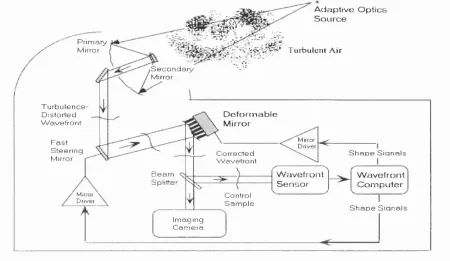
optics (AO) [52, 66, 64, 71, 88, 108]. Figure 1.1 shows a schematic diagram of an

adaptive optics system.

A d a p tiv e O p tic s S o u r c e

P r im a r y

M irr o r T u r b u le n t A ir

S e c o n d a r y M irr o r

T u r b u le n c e -D is to r t e d W a v e f r o n t

D e f o r m a b le M irror

M irro r D r iv e r

F a s t S te e r in g

M irr o r C o r r e c te d_{W a v e fr o n t} S h a p e S iq n a ls W a v efro n t

S e n s o r B e a m

S p litte r

W a v e fr o n t C o m p u t e r

M irro r

D r iv e r C o n tro l_{S a m p le}

S h a p e S iq n a ls Im a g in g

C a m e r a

Figure 1.1: Schematic diagram of an adaptive optics system. (From http:/www. aoinc.com/AOS/Aotutorial.html: reprinted with permission from Adaptive Optics Associates, Inc. a unit of Hamilton Standard, a UT co. (1997))

turbulence compensation for astronomy [108].

1.2

A d a p tiv e Secon d ary M irror

Conventional adaptive optics operate like auxiliary instruments and are more or less independent of the telescope. A typical system (figure 1.1) uses additional relay optics to form an image of the telescope’s pupil or an image conjugated with a nominal turbulent layer(s) in the atmosphere on a deformable mirror(s) mounted on an optical bench. The system usually also includes a separate mirror for removing the tip /tilt component of the wavefront distortion. Further reimaging optics are then required to bring the light to a focus on the science and wavefront sensing cameras.

Adaptive S econdary Mitror

Control System

5 W C W laser turned to 5 8 9 .0 nm

Science Instrum ent R eference star

Tilt Detector

W avefront Sensor

Figure 1.2: Schematic of the adaptive secondary mirror system in the 6.5 m Multi- Mirror Telescope (MMT) adaptive optics [81]

secondary approach needs no extra relay or reimaging optics, the approach has sev­ eral advantages compared to the conventional approach: 1) optical throughput is greatly enhanced, 2) negligible extra IR emissivity is introduced, which is a crucial advantage for a system intended to operate primarily in the infrared and 3) no ex­ tra polarisation is caused. Figure 1.2 shows a schematic diagram of the adaptive secondary mirror system of the 6.5 m Multi-Mirror Telescope (MMT) [81].

1.3

T h e A u th o r ’s C o n trib u tio n s and C o n ten ts o f

th e T h esis

grant. Optical test equipment was procured under the UK Higher Education Fund­ ing Council (England) Joint Research Equipment Initiative Scheme.

1 .3 .1

T h e A u t h o r ’s C o n tr ib u tio n s

When the author joined the project in September 1995 as part of international col­ laboration between KAIST and UCL, Bigelow [10, 11] had finished the preliminary or conceptual design of the demonstrator and identified some commercial compo­ nents for the system. He had then left the OSL to join the Observatories of the Carnegie Institute of Washington, USA.

The project has been progressed under the author’s full responsibility from the very beginning of the author’s joining. The author’s contribution to the ASM project can be summarised as follow:

• Re-comparison analysis of the MMT AO system and the William Herschel Telescope (WHT) AO system in terms of throughput, emissivity and polari­ sation

• Defining the technical and operational requirements of the project • Detailed mechanical design of all parts

• Extensive Finite Element Analysis (FEA) of the dem onstrator

• Theoretical analysis of the dem onstrator’s ability to compensate the atmospheric induced distortions

• Production and analysis of the drive electronics designed by G. Nixon at the OSL

• Development of assembly and disassembly techniques

• Development of on-off procedures to preserve the optical quality of the demon­ strator even when the power is off

• Static testing of the demonstrator

• Extension of simulation and experiments on the OSL/SIRA wavefront sensor

• Dynamic testing of the demonstrator

• Control and interface software development

1 .3 .2

C o n te n ts o f t h e T h e s is

The contents of the thesis, by chapter, are as follow.

• Chapter 2 presents a summary of adaptive optics systems and the character­ istics of atmospheric turbulence.

• Chapter 3 introduces the concept of adaptive secondary mirrors and reviews the current research on deformable secondary mirrors in the world and at the OSL.

• Chapter 4 examines design considerations and presents detailed design work for the dem onstrator and for its drive electronics.

• Chapter 5 describes the results of performance analysis of the dem onstrator using FEA.

• Chapter 6 presents the building of the dem onstrator and details the results of testing programs to characterise each component.

• Chapter 7 provides the results of the laboratory performance tests of the demonstrator.

C hapter 2

W h at is A d ap tive O ptics?

2.1

A d a p tiv e O p tics S y ste m s

An adaptive optics system could be defined as a system which removes or improves the wavefront distortions introduced by the earth ’s atmosphere by means of an optical component introducing a controllable counter wavefront distortion which both spatially and temporally follows th at of the atmosphere [64]. An adaptive optics system usually consists of four components; 1) an astronomical reference source known as a guide star^ 2) a wavefront sensor to measure the distorted wavefront, 3)

a wavefront correction device to produce the wavefront correction (usually including

a separate steering mirror to remove the tip /tilt component) and 4) a control system

to calculate and apply the necessary drive signals to the wavefront correctors. The AO system delivers the corrected output to a scientific instrum ent to record the data from the astronomical object of interest.

A variant of the system described above is a multiconjugated adaptive optics system

2 .1 .1

G u id e S ta rs

Adaptive optics systems are designed to compensate turbulence-distorted wavefronts continuously and independent of the direction of the observation in the sky. A sufficiently bright guide star must then be available within the isoplanatic angle

(see section 2.2.4) around the astronomical object being observed. However, it is not always possible to find a sufficiently bright guide star close to an arbitrary astronomical object (table 2.2) and this limits the achievable sky coverage of an AO system.

The situation is improved by observing astronomical objects in the infrared (IR) rather than in the visible part of the spectrum (section 2.1.5 and 2.2). In the infrared, the isoplanatic angle is bigger and the spatial and tem poral sampling of the wavefront can be reduced for a given image quality. Therefore, most astronomical adaptive optical systems intend to operate in the far-red or near infrared part of the spectrum, with only partial correction in the visible [13, 40]. In many cases, the sensor uses the visible light to detect the wavefront while the science instrum ent operates in the infrared, an approach which is known as polychromatic wavefront

sensing [64].

Another promising way to overcome the sky coverage limitation is the use of artificial

reference stars, also referred to as laser guide stars, laser probes and laser beacons.

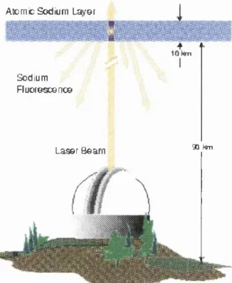
This was proposed by Feinleib in 1982 [58] and independently discovered by Foy and Labeyrie in 1985 [101]. The artificial star is generated using a laser either by Rayleigh backscatter from heights lower than 20 km or by spontaneous emission from Na atoms located in a layer at % 90 km. Such an artificial reference star can be created as close to the astronomical target as desired and a wavefront sensor measuring the returned laser light can be used to correct the wavefront aberrations of the target object. Figure 2.1 illustrates the use of mesospheric sodium as an artificial reference star for adaptive optics in Los Almos Laboratory.

Nevertheless, the dissimilarity in range between the laser guide star and the object leads to errors in the measurement of the aberrations known as focal anisoplanatism

Atomic Sodium Layer

Sodium Fluorescence

90 Wn

Laser Beam

Figure 2.1: Schematic illustration of the use of mesospheric sodium as an artificial star for adaptive optics, (from h ttp ://t4 .lanl.gov/pwm /adaptive.htm l: with permis­ sion from P. Milonni)

as on the way down, whereas the star light only traverses its path once, the artificial star can not be used to measure the tip /tilt component of the seeing. The prob­ lem can be solved by using a separate natural guide star to determine the tip /tilt component of the wavefront distortion. This still leads to an improvement in the sky coverage because i) only the tip /tilt is being measured therefore a much fainter guide star is needed than with a wholly natural guide star system, ii) the star can be further from the astronomical object of interest since the tip /tilt of the wavefront is correlated over a wider angle than higher order aberrations and iii) the image of the star will be also improved by the adaptive correction for scientific objects.

2 .1 .2

W avefron t S en sors

Unsampled ^ Turbulence

above \

Beacon

Incorrectly M easured"" Turbulence

r guide star)

# -, fV &

T elescop e with Adaptive Optic*

is to measure the distortions. Several astronomical wavefront sensors have been proposed or used: 1) the shearing interferometer [18, 70], 2) the Shack-Hartmann wavefront sensor [26, 28], 3) the pupil-imaging wavefront gradient sensor [90], and 4) the curvature wavefront sensor. The first three sensors measure wavefront tilts (gradients) while the last one measures curvature directly.

Shearing interferometer wavefront sensors work by comparing two copies of the

wavefront shifted (sheared) laterally or radially by a small amount relatively to each other. Since the separation of the fringes is proportional to the wavelength used, gratings are commonly used to perform the shear which is also proportional to the wavelength. Therefore the resultant separation of the fringes generated by gratings is independent of the wavelength. Thus the sensor can be used with a broadband, white-light signal. It is necessary to make at least two orthogonal measurements to assess the full wavefront.

The Shack-Hartmann or Hartmann-Shack wavefront sensors are particular forms of

the H artm ann sensor and are the most commonly used in adaptive optics (figure 2.3). The traditional Hartm ann screen in the pupil is replaced by an array of small lenslets at a conjugate to an image of the pupil or deformable mirror. Each lenslet forms an independent image of the incoming wavefront. Shifts in the positions of these images can be shown by simple geometric optics to be proportional to the mean wavefront gradient over each lenslet. It is not necessary to divide the light into two as is the case for shearing interferometer devices and almost all the light collected is used for wavefront measurement.

Pugh [90] in 1995 proposed a new approach to wavefront sensing called pupil-imaging

wavefront gradient sensing. It has a simple sensor configuration (figure A .l) which

Ray

Directions

Incoming

W ave

Lenslet

Array

üubaperture

2-Dimensional

Detector Array

I _ Spot

Deviation

Figure 2.3: Schematic diagram of H art maim- S h ack wavefront sensor. (From http: / www.aoainc.com/AOS/Aotutorial.html: reprinted with permission from Adaptive Optics Associates, Inc. a unit of Hamilton Standard, a UT co. (1997))

The curvature wavefront sensor was proposed and developed by Roddier [91, 92,

94]. The sensor compares the illumination patterns in two extra-focal images and measures the local wavefront curvature. In principle, the signal from a curvature sensor then can be amplified and directly applied to membrane or bimorph mirrors. Although in practice every one needs control system because no system behaves ideally, the combination of wavefront curvature sensing and bimorph can still result in substantial advantages in the control of the adaptive optics system. However, this is not the case for many other adaptive optics systems, where the curvature signals have to be converted into the tilts or phase signals.

2 .1 .3

W avefron t C o rr ectio n D e v ic e s

of propagation. At the present time, reflective devices (i.e. mirrors) are the most successful and generally used.

Many types of correction devices have been developed and used to m atch the wave- front distortion under varying conditions. These can be categorised into four types: 1) segmented mirrors, 2) continuous thin-plate mirrors, 3) bimorph or membrane mirrors and 4) other types.

Segmented mirrors providing tilt or both piston and tilt capability have been used

in a number of systems [25, 56, 79]. From the optical design point of view, the use of segments providing both piston and tilt capability is preferable to piston-only cor­ rection because fewer segments are required to match a given wavefront. Segmented mirrors have some advantages compared to the other types: 1) the mirrors can be controlled directly from tilt-sensing wavefront sensors, and 2) segmented mirrors can provide a better fliting performance than a continuous facesheet mirror when coupled to a Shack Hartm ann wavefront sensor. However the gaps between the segments cause concerns because of light loss, extra infrared therm al emission, and scattering of light. The former two effects are less im portant for solar observations th an in other astronomical observations. Therefore segmented mirrors have been used in solar AO systems [25] while continuous faceplate mirrors have been mostly chosen for non-solar AO systems.

The continuous thin-plate type with discrete actuators is widely used for active or

adaptive mirrors in the medium size range from about 10 cm up to 2 m in diam­ eter [15, 33, 67, 106] and only for active mirror in the large size range above 2 m in diameter. Deformation of a thin-plate requires an array of actuators located at discrete points. The deformation of the mirror by a single actuator is called the in­

fluence function (IF) of the actuator. The actuators may exert either forces normal

/

G lass

Piezo-electric material

Electrod e s

Figure 2.4: Cross section of a bimorph deformable mirror

mirrors while position actuators are used for small mirrors in which the provision of the necessary backing plate stiffness and stability is not a great problem. In the bending case, the use of bending moments allows the deformation of the mir­ ror without reaction forces from a backing plate and therefore a lighter mechanical structure can be used.

2 .1 .4

W a v efro n t C o n tr o l S y s te m

Closed loop adaptive optics systems must compensate for time-varying wavefronts on the basis of noisy and finite sensor measurements. The control system should calculate from the wavefront sensor measurement the command sent to the actuators of the deformable mirror. The calculation must be done quickly (up to 1000 Hz) (See 2.2.2), otherwise the state of the atmosphere may have changed rendering the wavefront measurement inaccurate.

There are two types of compensation techniques: modal [73] and zonal [23] correc­ tion. In modal correction the wavefront signal is expressed by a linear combination of modes of a set of basis functions such as the Zernike polynomials. Usually some of the modes are corrected depending on the image quality requirement and the design considerations. On the other hand, in zonal correction, each zone/ segment/ mirror element is controlled independently in a manner analogous to a phased array. The correction will be imperfect because of the finite size and number of sensors, measurement noise, the finite number of degrees of freedom in the correction and possible deficiencies in the control law [39, 103]. The control systems try to minimise the imperfection based on a figure of merit {merit function), which is a numerical representation of how closely an optical system meets a specified set of goals [121]. There are several types of merit functions: 1) the Strehl ratio which is the ratio of the peak intensity of a point image to the peak intensity of the point image formed by a perfect aberration-free system, 2) the Full-Width Half-Maximum (FWHM) which is the w idth across the profile of a point image at half maximum value of its peak, 3) the encircled energy which represents the percentage of the total energy in a point image which is contained within a given diameter which is usually the diam eter of the Airy disk and 4) the en-rectangled energy which represents the percentage of the to tal energey in a point image which is contained within a form of rectangle. Strehl ratio is a good measure of image quality when the optical system is well corrected [117]. The relation between Strehl ratio and the root-mean-squared (RMS) optical path difference(OPD) is well approximated by

squares fitting techniques to optimise the Strehl ratio by fitting the optical compo­ nent shape to the wavefront signal pattern [14, 35]. An adaptive optical system can also be controlled by a neural network where the neural control perm its a direct conversion of the intensity distribution measured in the near field into the control signals of a wavefront corrector [48].

2 .1 .5

W a v e le n g th

Electro-magnetic (EM) radiation from the sky includes not only visible light, but also infrared radiation, microwaves, radio waves, ultraviolet lights and X-rays. EM radiation is generated by processes which occur at various energies. There is much unique information to be gained from observations in different wavelength ranges. For example, extremely hot m atter with tem peratures of millions of degrees such as gigantic explosions can be observed only in the ultraviolet or X-ray whilst extremely cool stars can be observed in the infrared [49, 96]. Star formation and the formation and evolution of galaxies also can be studied in the infrared [7].

Certain portions of the EM spectrum get absorbed or blocked by the atmosphere while the rest can get through the atmosphere, at least partially. The spectral band over which the EM spectrum can get through the atmosphere is called the atmospheric window (figure 2.5). Optical light, which is not shown in figure 2.5, can travel nearly unimpeded through the atmosphere.

o

1 0 0

V

C C D

o

1 0 0 T

C H ^

----1 o

1 0 0 _... o

i , o o

O3 ----1 k o

1 0 0 " I f \ r

- - T y

CXD2

1 0 0

---1---— M 1 II

irfr-V

HD O

o

1 0 0 f ï i n y ' r '

HyD

o lOO

1 2 3 4 s e 7 8 S 1 0 11 1 2 1 3 1 4

A a g r a a a t a a b m a r p t ia n

1 6 W a v o l a n e t h

Figure 2.5: Infrared absorption by atmospheric gases, reproduced from S.L. Val- ley [97]

2.2

W avefront D isto r tio n B y th e A tm o sp h ere

When light passes through the earth’s atmosphere, the light is disturbed by the random refractive index inhomogeneities of the atmosphere. The disturbance takes the form of 1) distortion of the phase of the wavefront and 2) variations of the am­ plitude called scintillation across the wavefront. If the light is collected by a lens and brought to focus, the quality of the image formed is influenced by the distor­ tions. The scintillation causes random apodization which degrades the image [110]. However, the image quality is much less sensitive to 2) than 1). Moreover, these amplitude effects are uncorrectable with deformable mirrors. So only the effects of atmospherically induced phase errors are generally considered in planning and evaluation of adaptive optics system.

2 .2 .1

S p a tia l P h a s e V a ria tio n s

associated with the deformations are denoted by 0(x) and 0(x'), respectively, then the phase structure function is defined as

= < > (2.2)

where

r = |x — x'l (2.3)

and the brackets < > denote an ensemble average.

According to theory developed by Kolmogorov [5], the phase structure function at the entrance function of the telescope caused by so called Kolmogorov turbulence is

/ \ 5 / 3

D^(r) = 6 .8 8 (^ -j raxf (2.4)

where the coherence length or Fried parameter ro which depends on the wavelength (A) and zenith angle of the viewing path (() is given by

ro = 0.185\^/^{cosCŸ^HJcl{h)dh\ (2.5)

C^{h) is commonly referred to as the structure constant of refractive index variations

and it represents the average turbulence strength as a function of altitude h. An aperture of dimension ro produces a near-diffraction-limited image th a t appears to change position as the atmosphere evolves with time.

2 .2 .2

T e m p o r a l P h a s e V a r ia tio n s

Optical turbulence is induced by tem perature fluctuations produced by air velocity fluctuations [5]. The wind velocities, responsible for the atmospheric optical turbu­ lence, live longer th at the time it takes for them to move across the aperture of telescopes. So the turbulence can be described as a set of frozen layers th a t move across the aperture at speeds th at vary as a function of altitude. This is known as

Taylor’s Hypothesis [45].

Greenwood [24] derived a critical time constant tq, for the coherence length ro and the average wind velocity over which turbulence remains essentially un­ changed:

To % 0 . 3 1 4 - ^ (2.6)

where the average wind velocity V^ind is given by the following equation for velocities

v{h) varying with height (h).

-'—(S')'"

Greenwood also derived the 3 DB cutoff frequency response of a simple closed loop control system, called the Greenwood Frequency fg . It is generally taken to be

fa = 0 .4 3 ^ ^ ^ = 0.135/. (2.8)

r . with

/o = - (2.9)

'^O

For typical cases of astronomical imaging, fo is of the order of 10 to 100 Hz.

2 .2 .3

A tm o s p h e r ic T u rb u le n c e a n d Z ern ik e P o ly n o m ia ls

The phase-structure function D ^(r) describes the statistics of phase fluctuation. However, to understand more clearly the nature of the effects of wavefront defor­ m ation on an optical system, the information concerning the shape of the deformed wavefront should be obtained from the structure function.

A set of Zernike polynomials are commonly used in describing the shape of the wave- front deformation in unobscured, circularly symmetric optical systems [77]. Follow­ ing Noll [104], the Zernike polynomials Zj{n, m), in which n is the degree of a radial polynomial and m the azimuthal frequency of a sinusoidal/ cosinusoidal wave and the index j is a mode ordering number, are defined by

^even j = + l-R» W \/2 cos(m(9)

^odd j = y / n T Ï R n { r ) V 2 sin(m^)

Zj = y/n -f IR nir), m = 0

(2.10)

where

D m / ^ ^ ____t t_______________^ « - 2 3 (2 1 1 ^

^ s! [(n + m )/2 - s]! [(n - m )/2 - s]!

Noll’s definition gives logical ordering to the modes and allows the modal orthogo­ nality given by

n m Expression Name Residual Variance A j(rad^)

1 0 0 1 piston 1.030 { D/ r of / ^

2 1 1 2rcos9 tilt 0.582 (D/ro)^/^

3 1 1 2rsin9 tilt 0.134 {D/ro)^/^

4 2 0 \/3(2r^ - 1) defocus 0.111

5 2 2 \/6r^sin29 astigmatism 0.0880 [ D/ r o f / ^

6 2 2 y/6r^cos29 astigmatism 0.0648 (D/ro)5/3

7 3 1 \/8(3r^ — 2r)sin9 coma 0.0587

8 3 1 \/8(3r^ — 2r)cos9 coma 0.0525 { D/ r o f / ^

9 3 3 y/8r^cos39 trefoil 0.0463 { D/ r of / ^

10 3 3 y/8r^sin39 trefoil 0.0401 { D/ r o f / ^

11 4 0 \/5(6r^ — 6r^ + 1) spherical 0.0377

Table 2.1: The first 11 Zernike polynomial terms and the mean square residual errors for Kolmogorov turbulence after removal of the first j Zernike polynomials

where

W{r) = I /tt r < 1

0 r > 1 (2.13)

An arbitrary wavefront (j){r, 6) over a circular aperture of arbitrary radius (R) can be expanded as a linear sum of Zernike polynomials given by

4>{Rp,0) = Y^üj Zj {p, 9) ,

3

with p = r / R and the coefficients aj being given by

% = j d'^'rpW(p)4>{Rp,e)Zj{p,e)

(2.14)

(2.15)

2 .2 .4

A n g u la r Iso p la n a tism

An adaptive optics system compensates the distorted wavefront based on the mea­ surements of the turbulence-induced phase fluctuations across the aperture of the optical system. The perturbations are detected by measuring the shape of a wave- front from a reference star (section 2.1.1), which may coincide with or be adjacent to the scientiflc star.

In the later case, the light from the reference star and the science objects travel through different regions in the turbulence (flgure 2.2). So the distortions are only partially correlated, which means the possible degradation of the accuracy of the wavefront compensation in the adaptive optics system. However, there is an angular region over which the atmospheric wavefront disturbances can be practically con­ sidered identical [42]. The angular diameter of this region is called the isoplanatic

angle 6q which is given by:

00 = 0 .3 1 4 ^ (rad), (2.16)

where H is the average distance of the seeing layer or

The isoplanatic angle typically ranges from 1 up to 10 arcsec in the visible [41]. The size of the isoplanatic angle bounds the operation of adaptive optics system by two fundamental limitations. Firstly, the probability of flnding a reference star bright enough for an efficient wavefront sensing would be about 10“ ^ ~ 10“^ in the visible and would reach ~ 1, only when the wavelength is larger th an 5 fim [102]. Even when a laser guide star is used as the reference source (section 2.1.1), a natural star is still needed to measure the tilt which can not be measured with such an artiflcial star. Secondly, the fleld of view in which the correction is performed is limited by the isoplanatic angle.

, - 1 6 1

, - 1 7 1

O

, - 1 8 1

, - 1 9 1

20

H e ig h t (km )

Figure 2.6: Time averaged C^(h) profile given by Valley [44] with height h (km):

C^{h) = (2.05 X h^^exp{—h) + 0.93 x 10~^^exp{ — h /1 .5 ))n ~ ‘^^^

technique to sense the position and contribution to the wavefront distortion of each turbulent layer.

2 .2 .5

C^{h)

V a ria tio n w ith H eig h t

To derive numerical values for the turbulence parameters, the profiles for turbulence or the structure constant of refractive index variations as a function of height must be established.

Figure 2.6 shows the model of turbulence given by Valley [44]. This model represents the time averaged C^{h) profile. The actual C^{h) profile varies temporally and from site to site. The curve in figure 2.6 does not show the rapid fluctuations in

C^{h) shown by Talion [83]. However, the model is often taken to be representative

Spectral Band A {^lm) ro (cm) To (sec) Tdet (sec) ^0 (arcsec)

Sky Coverage (%)

U 0.365 9.0 .009 .0027 7.4 1.2 1.8 E-5 B 0.44 11.5 .011 .0034 8.2 1.5 6.1 E-5 V 0.55 14.9 .015 .0045 9.0 1.9 2.6 E-4 R 0.70 20.0 .020 .0060 10.0 2.6 0.0013 I 0.90 27.0 .027 .0081 11.0 3.5 0.006 J 1.25 40 .040 .0120 12.2 5.1 0.046 H 1.62 55 .055 .0164 13.3 7.0 0.22

K 2.2 79 .079 .024 14.4 10.1 1.32

L 3.4 133 .133 .040 16.2 17.0 14.5

M 5.0 210 .21 .063 17.7 27.0 71

N 10 500 .50 .150 20.4 64 100

Table 2.2: Values for ro, /g , for various wavelengths with limiting V magni­ tude for polychromatic wavefront sensing and sky coverage at average Galactic lat­ itude, reproduced from Beckers [64]. Conditions are: 0.75 arcsec seeing at 0.5

T'det = O.Stq; Vyjind = lOm/scc; 5000 m; photon detection efficiency (includes

transmission and quantum efficiency) = 20%; spectral bandwidth=300 nm; Signal to Noise Ratio (SNR) = 100 per Hartmann-Shack image; detector noise = 5e“ .

Table 2.2, reproduced from Beckers [64], lists a range of values for coherence length ro. Greenwood frequency /g , and isoplanatic angle 6q for several wavelengths. The values were computed using a wind velocity of 10 m /s and an average turbulence height of 5000 m. This table also shows the reference star limiting m agnitude for wavefront sensing in a polychromatic wavefront sensing mode (section 2.1.1) for the different photometric bands. The resulting sky coverage was derived taking into consideration the isoplanatic angle size 6q and the number of stars per unit area of

Scientific programmes Prime Band

Field of View

Magn. Range

Besoin (arcsec)

Desirable Strehl Ratio Images:

Brown Dwarfs and M stars H < 10" 12-20 0.1 0.5 Young Stellar Object Disks H < 10" 12-20 0.1 0.5 Planet Searches H < 5" 20-29 - 0.5

Local Group Star Clusters K 20" 20-26 < 0.1 0.3 G ravitational Arcs H 20" 19-34 < 0.1 0.3

Spectra:

Studies of Star Formation K 20" - < 0.1 0.5

Local Group Old Stars K 10-20" 20-23 < 0.3 0.3 Galaxy Nuclei Dynamics K 10" 14-17 < 0.1 0.3 Starburst Galaxies K 20" 19-23 < 0.3 0.2 Gravitational Arcs H 20" 19-23 < 0.1 0.3

Table 2.3: High priority science cases for the Gemini AO [112]

2.3

S cien tific D rivers for A d a p tiv e O p tics

Since AO for astronomy has been developed to provide useful information to as­ tronomers, it is im portant for the design and performance of an AO system to be driven by science rather than technology. It is therefore worth reviewing the scien­ tific drivers for AO systems.

C hapter 3

W h y A d ap tive Secondary

M irrors?

3.1

T h r o u g h p u t, E m issiv ity , an d P o la r isa tio n C o m ­

p a riso n

An adaptive secondary mirror, unlike conventional adaptive optics systems, does not add any polarisation, reflective losses, and emissivity. This section lists the results of a comparison analysis between the W HT AO system and an adaptive secondary mirror system for the MMT conversion (figure 1.2) in terms of throughput, emissivity, and polarisation. The respective minimum numbers of surfaces for the two systems, excluding the telescope primary and secondary mirrors, were from Bigelow [10] and are shown in table 3.1.

This analysis was originally performed by Bigelow [10]. Figure 3.1 plots the reflec­ tivity d ata for over-coated silver which he used in the analysis, from 0.32 /im to 0.82 fim, and the resultant total reflectivity after multi (3, 5, 10, 15, and 20) reflec­ tions / refractions. He also calculated the infrared (0.7 - 20.0 fim) to tal reflectivity and emissivity for multiple reflections and two reflectivity values (99% and 98%), which are tabulated in table 3.2.

Optical Path Reflections Refractions total Surfaces WHT Nasmyth system:

Tracker 8 12+ 20+

WPS 7 9+ 16+

Science 5 5+ 10+

MMT Adaptive Secondary:

Tracker - 3+ 3+

WPS - 3+ 3+

Science - 2+ 2+

Table 3.1: Reflecting and refracting surfaces counts for the WHT and MMT AO systems, Reproduced from Bigelow [10]

0.9 0.8 0.7

0.6

<u cc

0.4 0.3

0.2

0.1

750 800

700 650

500 550

W a v e l e n g t h (n m ) 600 450

400 350 300

Figure 3.1: Bigelow’s results on total reflectivity for multiple reflections (1, 3, 5, 10, 15, and 20) [10]

Reflectivity Surfaces _Rto t a l{%) Emissivity (%)

99% 3 97.0 3.0

99% 5 95.1 4.9

99% 10 90.4 9.6

99% 15 86.0 14.0

99% 20 81.8 18.2

98% 3 94.1 5.9

98% 5 90.4 9.6

98% 10 81.7 18.3

98% 15 73.9 26.1

98% 20 66.8 33.2

Table 3.2: Bigelow’s results on total infrared (0.7-20.0 f i m ) reflectivity Rt o t a l and

emissivity for multiple reflections and two reflectivity values (99 % and 98 %) [10]

3 .1 .1

T h r o u g h p u t

Throughput is a measure of the amount of light th at is transm itted through an

optical system. In polychromatic sensing, the light in the infrared band is used for the scientific measurement while the light in the visible band is used for the wavefront sensing. Therefore the throughput in both bands, which determines the amount of the light for scientiflc measurement and wavefront sensing, is a key param eter of the ASM.

The comparison was performed based simply on the number of optical surfaces in the system. D ata on the reflectivity of over-coated silver coating was obtained from a commercial product catalog [29] (flgure 3.2(a)). Reflectivity d ata for an anti-reflection coating for refracting optical surfaces was obtained from the same catalog [29] (flgure 3.2(b)). The incident angle was assumed to be zero for the simplicity of calculation as this only marginally effects the resulting values.

100

a ) W a v e le n g th in m ic ro n s

6 0 0 6 5 0 7 0 0 7 5 0

b ) W a v e le n g th in n an o m e te rs

8 5 0

Figure 3.2: a) Reflectivity (%) of overcoated silver coating [29] b) Reflectivity (%) of broadband multi-layer anti-reflection coatings [29]

respectively.

The WHT system will lose 17 % and 6 % of the original flux for the wavefront sensor (at 0.7 /im) and for the science instrument (at 2.2 //m) respectively, whilst the MMT AO system will lose less than 1 % of the original flux in both. The 17 % loss of the WHT system for the wavefront sensor is better than the result of Bigelow’s analysis i.e. 35% loss (see flgure 3.3). This is because he used the reflectivity data of over­ coated silver for refraction in the visible bands which has lower value than th at of the multi-layer coating (flgure 3.2).

For the same amount of total flux in the wavefront sensor, the WHT needs a 20 % brighter guide star to compensate for the 17% loss of the original flux. Since the apparent magnitude of a star m y is a logarithm of the brightness of the star bm as

given by

Ol CD C3 o 100 90 80 70 60 50 4 0 30 20 10 0 100 95 /

... - 90 T "

---\ /

/ \ 85

& 80

S 75_CD

65

60

55

50

0.6 0.7 0.8

W a v e l e n g t h in m i c r o n s

2 1 2 2 2 3

W a v e l e n g t h in m i c r o n s

Figure 3.3: Total throughput (%) for the MMT and WHT AO systems in polychro­ matic wavefront sensing, a) For wavefront sensing (centred at 0.7 iim) b) For science instrument (centred at 2.2 fim). The solid and dotted lines represent the results of the author and Bigelow [10, 11], respectively.

will the difference between the minimum stellar magnitudes for the WFIT and the MMT. When the original reflectivity has deteriorated by 4%, the total losses will become 60% for the WHT system and 12% for the MMT system. The difference would then approximately correspond to one stellar magnitude.

The required magnitude for a natural guide star is determined by many factors including the level of adaptive compensation, the telescope aperture size, and the properties of the WFS detector. However, the loss of one stellar magnitude will significantly reduce the number of astronomical objects accessible to the AO system and hence the science instrument it feeds.

3 .1 .2

E m iss iv ity

Light not transm itted or reflected by the optical surface in an AO system is absorbed and re-emitted as thermal radiation. For infrared observations, emissivity in the optical train will reduce the signal-to-noise ratio (SNR) in the final image.

20

18 16 14

g 12

10

CO CO

s 8

6

4 2 0 2 .0 5

WHT AO

MMT AO

2.1 2 .1 5 2.2 2 .2 5

W a v e le n g th in m ic ro n s

2.3

Figure 3.4: Emissivity (%) for MMT and WHT AO systems for science instruments (around 2.2 (im)

about the AO system optics, temperatures, baffling, and the surrounding environ­ ment. A comparison was therefore performed simply based on the number of optical surfaces in the system. The analysis also assumed that all energy not reflected during reflection and not transm itted during refraction is absorbed and re-emitted.

Figure 3.4 shows emissivity of MMT and WHT AO systems for science instruments. The total emissivity for the WHT system is 6% while th at for the MMT system is smaller than 1 %. Note that the Gemini telescope requirement [82] for total IR emissivity is 4%, with a goal of 2%. The WHT AO system will introduce more than one and half times the Gemini emissivity requirement while the MMT AO system introduces a smaller IR emissivity than the goal of Gemini telescopes. (Total emissivity of the telescope and AO system in the K band must be less than 19%, with a goal of this emissivity to b/im.)