ORIGINAL ARTICLE
Optimization of Cutting Parameters
for Trade-off Among Carbon Emissions, Surface
Roughness, and Processing Time
Zhipeng Jiang
1, Dong Gao
1, Yong Lu
1*and Xianli Liu
2Abstract
As the manufacturing industry is facing increasingly serious environmental problems, because of which carbon tax policies are being implemented, choosing the optimum cutting parameters during the machining process is crucial for automobile panel dies in order to achieve synergistic minimization of the environment impact, product quality, and processing efficiency. This paper presents a processing task-based evaluation method to optimize the cutting parameters, considering the trade-off among carbon emissions, surface roughness, and processing time. Three objective models and their relationships with the cutting parameters were obtained through input–output, response surface, and theoretical analyses, respectively. Examples of cylindrical turning were applied to achieve a central com-posite design (CCD), and relative validation experiments were applied to evaluate the proposed method. The experi-ments were conducted on the CAK50135di lathe cutting of AISI 1045 steel, and NSGA-II was used to obtain the Pareto fronts of the three objectives. Based on the TOPSIS method, the Pareto solution set was ranked to find the optimal solution to evaluate and select the optimal cutting parameters. An S/N ratio analysis and contour plots were applied to analyze the influence of each decision variable on the optimization objective. Finally, the changing rules of a single factor for each objective were analyzed. The results demonstrate that the proposed method is effective in finding the trade-off among the three objectives and obtaining reasonable application ranges of the cutting parameters from Pareto fronts.
Keywords: Automobile panel dies, Carbon emission, Parameter optimization, Multi-objective optimization, NSGA-II
© The Author(s) 2019. This article is distributed under the terms of the Creative Commons Attribution 4.0 International License (http://creat iveco mmons .org/licen ses/by/4.0/), which permits unrestricted use, distribution, and reproduction in any medium, provided you give appropriate credit to the original author(s) and the source, provide a link to the Creative Commons license, and indicate if changes were made.
1 Introduction
In 2017, the total number of automobiles in China reached 217 million, and has shown an increasing trend each year [1]. In recent years, the upgrading of cars has accelerated which has caused an acceleration of the need for automobile panel dies. The design and manufactur-ing times of automobile panel dies accounts for 2/3 of the automobile development cycle [2], and therefore the pro-cessing efficiency and quality of the die directly restrict the speed of an auto body modification. There are large numbers of rotating machinery parts on the die. Turn-ing is a necessary process for the machinTurn-ing of rotary
parts, such as ejector pins [3]. However, carmakers have been striving to maximize profits, putting their economic benefit first and ignoring the environmental attributes of their products. Carbon emissions (C) are the major causes of global problems, such as the melting of the Arctic and Antarctic glaciers, rising sea levels, and global warming. To neutralize or alleviate the environmental pressure of carbon emissions, and to achieve the sustain-able development of the economy, society, and future generations, countries around the world have jointly for-mulated a series of environmental laws and regulations and related standards. The international community first enacted an environmental-related law (United Nations Framework Convention on Climate Change) in 1992 to meet the challenge of global warming. The enforcement of the Kyoto Protocol in 2005 marked the entry into a
Open Access
*Correspondence: [email protected]
1 School of Mechatronics Engineering, Harbin Institute of Technology, Harbin 150001, China
substantial phase of reducing greenhouse gases in the international community [4].
Lightweight design technologies used in machine tool structures, 3-R manufacturing, the application of new processing technologies and other aspects are potential measures for energy saving and a reduction of emissions in the manufacturing industry [5]. However, these meas-ures are difficult to apply widely within a short time.
There is a massive amount of existing machine tools in reserve, and parameter optimization for existing machine tools and processing technology is not only an effective way to improve the processing quality and efficiency [6], it is also an effective measure in energy saving and the reduction of emissions [7]. Therefore, parameter optimi-zation has become a hotspot in current research. Cam-patelli et al. [8] employed an experimental approach to model the energy consumption in the milling of AISI 1050 carbon steel, and claimed that increasing the mate-rial removal rate (MRR) as much as possible will help reduce energy consumption during the processing. Wójcicki et al. [9] adopted a model-based approach for a systematic energy efficiency evaluation and optimization during turning operations, combining a spindle, chiller, and material removal models, and taking into account the strong interrelations between the cutting process, a spindle with a permanent magnet motor, and its chiller. Zhong et al. [10] considered the effects of the cutting parameter combinations on the energy consumption at a certain material removal rate, and based on this dis-covery, considered a specific energy consumption as the optimization goal and took the cutting parameters as the optimization variables during the material removal pro-cess during the turning; cutting parameter sets with a large feed rate were then recommended. Bilga et al. [11] regarded the cutting speed, feed rate, cutting depth, and nose radius along with their interactions as the variables to optimize energy consumption, and showed that the feed rate is the vital dominating parameter for a reduc-tion of the energy consumed; however, the nose radius does not contribute much. To lower the specific cut-ting energy in high-speed milling, Wang et al. [12] took 7050-T7451 aluminum alloy as the processing object to reveal the influence of the cutting speed, undeformed chip thickness, and tool rake angle on the cutting energy consumption.
However, parameter optimization aiming at mini-mizing the environmental cost (energy consump-tion or carbon emission) often sacrifices the economy of the mechanical products, machining processes, or product performance. Therefore, parameter optimiza-tion constrained by multiple optimizaoptimiza-tion objectives has received increasing attention. Wang et al. [13] took energy consumption, cost, and surface roughness as the
inaccurate, and used three analysis methods (the RSM-based Goal Programming model, TOPSIS-RSM-based Taguchi approach, and Grey Relational Analysis-based Taguchi approach) to analyze the coupling relationship between cutting parameters and different tools (multi-coated TiCN+Al2O3+TiN, surface carbon coating, and dia-mond coating), and different materials (6061, 6082, and 7075). The results show that the RSM-based Goal Pro-gramming approach is generally better than the other two. Li et al. [22] used a multi-objective particle swarm optimization algorithm as a tool to minimize the energy and processing time simultaneously through the opti-mization of the cutting parameters during CNC milling, and pointed out that the width of cut is a major process parameter affecting both the energy and processing time. To address the problem of a simultaneous optimization of the cutting parameters and processes, Zhang et al. [23] used an improved universal gravity search algorithm to establish a two-part search space for the cutting param-eters and process layout, and proposed a target optimi-zation model for minimizing the processing time and carbon emissions.
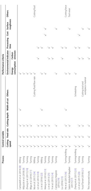
A comparison of the literature on the optimization of environmental indicators in recently published studies is shown in Table 1. Summarizing the findings of the thor-ough literature review above, it can be claimed that the current studies on parametric optimization for minimiz-ing the negative environmental influence present the fol-lowing shortages.
1. Numerous parameter optimization models only take energy consumption, carbon emissions, or other environmental indicators as the optimization objec-tive, which often sacrifice processing efficiency or product quality, and are extremely one-sided. To fully analyze the trade-offs among environmental, product quality, and efficiency indicators, for example, mini-mizing the carbon emissions and processing time and maximizing the product quality, multi-objective parameter optimization is worth studying.
2. The optimal parameters in many studies are directly derived from experimental parameter combinations, the results of which are extremely dependent on the selected experimental parameters. If the experimen-tal parameters are not chosen well, they are easily trapped into the local optimum.
3. In multi-objective optimization studies using carbon emissions as an indicator, the same cutting depth is often specified, or the carbon emissions are calcu-lated after a single cutting according to the orthogo-nal test table. Although the former applies the same processing tasks, it limits the cutting depth and the parameter optimization is not comprehensive. The
latter will result in a different amount of material removed owing to a different cutting depth, and the results lack comparability.
As shown in Table 1, energy consumption minimi-zation is usually selected as an environmental indica-tor in the literature. However, compared with energy consumption, carbon emissions can more fully reflect the environmental impact of the machining process, and are more in line with the actual situation. Surface roughness is one of the commonly used indicators for evaluating the product quality. Different surface rough-ness thresholds may cause large changes in the process-ing time, tool wear, carbon emissions, and other factors. The surface roughness is a reasonable indicator of the surface quality. The processing time largely determines the market competitiveness of the products and the ability to cope with market risks. It is also an important indicator used to measure the technical and manage-ment level of an enterprise. It is therefore reasonable to take lower carbon emissions, a lower surface rough-ness, and a lower processing time as the optimization objectives. In terms of the decision variable selection, cutting parameters directly affect the carbon emissions, surface quality, and processing time, and thus the cut-ting parameters were chosen as the decision variables. During actual processing, the workpiece material is often selected long in advance, and there is no need to apply an optimization. Cutting tools have an effect on the optimized targets and a particular optimization space [24], which can be used as one of the decision variables. However, in an investigation into the factory setting, it was found that the tool used is relatively fixed and that the tool parameters cannot be easily replaced. For the time being, however, this is not considered as a control variable in the present study.
Table 1 C omparison among the pr op osed optimiza
tion algorithm and other studies in the lit
er atur e Pr oc ess Con tr ol v ariable Per formanc e crit eria
Cutting speed
Feed r at e Cutting depth W idth of cut O thers En vir onmen tal indica tor Pr oc essing time Cost Sur fac e roughness O thers Ener gy consumption
Carbon emission
Campat
elli et
al
. (2014) [
8 ] M illing √ √ √ √ √ W ójcick i et al
. (2018) [
9 ] Tur ning √ √ √ √ Zhong et al
. (2017) [
10 ] Tur ning √ √ √ √ Bilga et al
. (2016) [
11 ] Tur ning √ √ √ √ M a et al
. (2017) [
24 ] M illing √ √
Cutting fluid flo
w rat e √ Cutting fluid Lin et al
. (2015) [
18 ] Tur ning √ √ √ √ √ Li et al
. (2016) [
22 ] M illing √ √ √ √ √ √ W ang et al
. (2014) [
13 ] Tur ning √ √ √ √ √ √ Li et al
. (2013) [
25 ] Tur ning √ √ √ √ √ Yi et al
. (2015) [
14 ] Tur ning √ √ √ √ Camposeco -Neg ret e (2015) [ 19 ] Tur ning √ √ √ √ √
Liu (2016) [
15 ] √ √ √ √ He et al
. (2017) [
16 ] Tur ning/milling √ √ √ √ √ √ Cutting f or ce
Salem Abdullah Bagaber (2017) [
17 ] Tur ning √ √ √ √ √ Tool w ear Zhang et al
. (2017) [
23 ] Tur ning/milling √ √ Scheduling √ √ Lin et al
. (2017) [
20 ] Tur ning √ √ √ √ √ √ Yusuf
Tansel (2018) [
between each objective and achieve a better surface quality, shorter processing time, and less environmental costs.
2 Methods
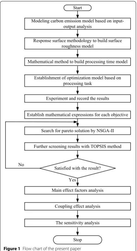
Facing increasingly severe environmental problems, the trade-off and restrictive relationship among the process-ing efficiency, processprocess-ing quality, and environmental impact were studied along with the optimization of the cutting parameters as decision variables to reduce the environmental impact, and improve the processing qual-ity and efficiency. First, existing optimization models of the cutting parameters when considering the environ-mental impact were analyzed, and it was found that the multi-objective optimization model is a popular but dif-ficult research topic. In view of the existing problems of this research, carbon emissions, the processing time, and the surface roughness were selected in this study as the optimization objectives, with the cutting parameters as the decision variables; RSM, NSGA-II, and TOPSIS as the technical means; and the processing task as the research object used to solve the multi-objective optimi-zation problem. Figure 1 shows the organization of the present paper.
First, three objective models and their relationships with the cutting parameters are needed, namely, the mod-eling carbon emissions model based on an input–output analysis to ensure the reliability of the system boundary, a response surface analysis to model the surface roughness to ensure the accuracy of the prediction, and a math-ematical method to build the processing time model to ensure the accuracy of the processing time calculation. The mathematical relationships used to establish the pro-cessing task-based multi-objective optimization model for high-efficiency, low carbon emissions, and high-qual-ity processing manufacturing are described in Section 3.
A turning case study is given in Section 4, and the multi-objective optimization equation is derived accord-ing to the experiment results.
The results and a discussion of the optimal Pareto solu-tions are presented in Section 5. NSGA-II was selected as the multi-objective optimization method to obtain the Pareto frontier. The optimal solution was obtained by sorting the Pareto solution set based on TOPSIS. A main effect analysis was carried out to find the ranking of significant factors. Contour maps were drawn through a simulation analysis to analyze the interaction between the decision variables and optimization objectives. Sub-sequently, a sensitivity analysis was carried out to analyze and explain the changing rules between the objectives and decision variables.
Finally, some concluding remarks are given.
3 Multi‑Objective Optimization Model 3.1 Decision Variables
In this study, the traditional turning process was selected as the research object for multi-objective optimization research, although the research method and theory can be applied to other machining processes. As mentioned in Section 1, the spindle speed, cutting depth, and feed rate were selected as decision variables.
3.2 Targets to be Optimized
3.2.1 Carbon Emission
An input–output analysis was originally applied to the field of economics, and the concept was quickly applied to other areas, playing an important role in describing the relation-ship between the final demand and total outputs from an
Mathematical method to build processing time model
Establishment of optimization model based on processing task
Experiment and record the results
Establish mathematical expressions for each objective
Search for pareto solution by NSGA-II
Further screening results with TOPSIS method
Main effect factors analysis
Modeling carbon emission model based on input-output analysis
Coupling effect analysis Start
Response surface methodology to build surface roughness model
Satisfied with the result?
Yes No
The sensitivity analysis
Stop
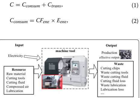
up-down perspective. The carbon emission model of the machine tools used during the cutting process should not only consider the carbon emissions produced by electric energy consumption, but also the carbon emissions pro-duced by auxiliary equipment, tools, and cutting fluid. An input–output analysis is used to analyze the carbon emissions during the machining processes to ensure the accuracy of the carbon emission calculation, as shown in Figure 2. The machining process requires the input of power and resources, in addition to the target products, and is also accompanied by a large amount of waste gen-erated at the output. According to the consumption form of the energy resources used during the machining process, carbon emissions are divided into consumable and trans-ferable carbon emissions. Consumable carbon emissions refer to carbon emissions from the electricity consumed during the machining process. The use of electricity does not produce carbon emissions, but the production process of electricity does. Carbon emissions from electric power are obtained by multiplying the electricity consumption by the electricity carbon emission factor (Eq. (2)). A calcula-tion of the electricity consumpcalcula-tion of CNC machine tools can be found in a previous study [26]. Transferable car-bon emissions refer to the carcar-bon emissions transferred from raw materials, cutting tools, cutting fluids, and other resources during the processing, which are transformed into waste materials such as chips, scrap cutting tools, and scrap cutting fluids. That is, transferable carbon emissions include two parts: input resource carbon emissions and output waste carbon emissions. As the calculation method, the mass/volume is multiplied by the carbon emission coef-ficient. Products are effectively exported, regardless of the carbon emissions produced. Because a processing task-based optimization model is adopted in this paper, the amount of material removed is also fixed, which cannot and does not need to be optimized. Therefore, this part of the carbon emissions is not calculated in this multi-objec-tive optimization
(1) C=Cconsum+Ctrans,
(2) Cconsum=CFene×Eene,
3.2.2 Surface Roughness
The formation of the surface roughness during the mechan-ical cutting process can be roughly summarized into three factors: geometric factors, physical factors, and vibrations of the process system. Geometric factors refer to the residual area of the cutting layer left behind on the machined sur-face when the tool moves relative to the workpiece. Many theoretical surface-quality calculation models are calcu-lated based on this characteristic [27]. The actual surface roughness after cutting has a large difference from the theo-retical roughness, which is mainly affected by the physical properties of the material being processed and the cutting mechanism. During the cutting process, the edge fillet of the tool and the flank surface will be plastically deformed by pressing and rubbing against the workpiece. The higher the toughness, the greater the plastic deformation of the material, allowing built-up edge and scale to easily appear, seriously deteriorating the roughness. The vibration of the processing system, such as the cutting parameters and the cooling lubricants, is an important factor affecting the sur-face roughness, and is an important means to control and improve the surface roughness during actual cutting. In this paper, the quality of dry turning is improved by chang-ing the cuttchang-ing parameters. For dry turnchang-ing, in this study, the machining quality is improved by changing the cutting parameters. Because the surface roughness of the workpiece is a non-linear process, a second-order polynomial response surface mathematical equation is utilized, as shown in Eq. (6), and the coefficients of the function can be obtained using the least squares method.
where h represents the turning parameters (spindle speed, feed rate, and depth of cut), β is the coefficient of
each term, and ε is a residual error.
3.2.3 Processing Time
Taking machine tools as a whole as the research object, the machining processing time Tmachin refers to the time required to complete the processing of a part, which con-sists of the maneuver time (also known as the basic time)
tmaneuver and auxiliary time tauxiliary.
(3) Ctrans=Cresource+Cwaste,
(4)
Cresource=Ctool+Ccool+Cair,
(5) Cwaste=Cchips+Ctool−w+Ccool−w,
(6) Ra=β0+
i
βihi+
i<j
βijhihj+
i
βiih2i +ε,
(7) Tmachin=tauxiliary+tmaneuver.
Waste Cutting chips Waste cutting tools Waste cutting fluid Cutting fluid loss Waste lubrication Lubrication loss Resource
Raw material Cutting tools Cutting fluid Compressed air Lubrication
Production
effective output
machine tool
Input Output
Electricity
The maneuver time tmaneuver is the cutting time needed to directly change the size, shape, and surface quality of the workpiece, including the stand-by time and idle run-ning time.
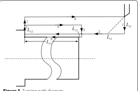
The idle running time, tidle , is determined as indicated in Figure 3.
The auxiliary time tauxiliary is the time consumed by
various auxiliary actions used to process each workpiece during a certain process, such as starting and stopping the machine tools, changing a tool, trial cutting, meas-urements, and other related steps consuming auxiliary action time. In this study, AISI 1045 steel was processed, and the processing task was small. It is considered that the auxiliary times of each group of processing tasks are the same, and thus there is no room for optimiza-tion, which can be omitted for convenience, and that the stand-by time is the same.
According to the generalized Taylor formula [28], the tool life is as shown in Eq. (12):
(8) tmaneuver =tstand−by+tidle+tcut.
(9) tidle=max
Lx1
vfx ,Lz1
vfz
+ N
j=1 L
z2j vf
+Lx2j vf
+Lz3j+Lz2j vfz
+Lx2j vfx
+max
L x1−Lx2
vfx
,Lz1+Lz2+Lz3 vfz
,N=1, 2, 3,· · ·
Lx2j=Lx2+j·ap.
(10) tcut =
N
j=1
Lz3j vf
,N=1, 2, 3,· · ·
(11) tauxiliary =tclam+tset+tpro+
tchan·tcut Ttool +tunl.
3.3 Constrains
For the diversity of the materials to be processed, the pro-cessing equipment, and fine and rough propro-cessing tech-nology, the proper values of the cutting parameters will be within a different interval. At the same time, the range of the cutting parameters will be defined by the proces-sors based on personal experience. Therefore, for the spe-cific practical machining process, the cutting parameters should be restricted to a certain scope to avoid unneces-sary calculations and a waste of resources.
Combined with the above research, a multi-objective optimization equation is obtained.
4 Case Study
4.1 Experiments and Data Acquisition
The turning process was taken as the research object. The experimental scenarios were carried out on a SMTCL CAK50135di CNC lathe with a spindle power of 6.5 kW, and its maximum spindle speed can reach 1450 r/min. The fast forward speed of the machine tool is 1900 mm/ min. A carbide cutting tool was employed for the experi-ment. The cutting tool material is YT15 and the rake angle is 10°, the main cutting-edge angle is 75°, and the tool tip radius is 1 mm. Some AISI 1045 steel bars with dimen-sions of φ90 × 120 mm were employed. The hardness of the steel is 187 HB, and its composition is 0.42%–0.50%C, 0.50%–0.80%Mn, 0.17%–0.37%Si, and ≤ 0.25%Cr [29].
The experimental setup is shown in Figure 4. The power requirement during the mechanical machining process was measured using a WT333 type digital power meter (Yokogawa). The measurement software provided by the manufacturer is WTViewerFreePlus. This type of measurement equipment can be used to measure all AC and DC parameters; moreover, integral and harmonic measurements can be conducted at the same time with-out changing the measurement mode. The limits of the measured current can be as low as 50 μA and as high as 40 A. The sampling frequency is 10 Hz, and the read-ing accuracy is 0.1%. For a more detailed description of the experiment, refer to our previous study [26]. A sur-face roughness measurement was conducted using a Tr200V1.5 surface roughness meter (Beijing Times Rui Da Technology Co., Ltd.) with a range of 0.005–80 μm.
(12)
Ttool =
A1/m vm
c ·axp/m·fy/m
.
(13)
min{C,t,Ra},
(14) s.t.,
nmin≤n≤nmax, fmin≤f ≤fmax,
ap−min≤ap≤ap−max.
1 x
L
1 z
L 2
x
L
3 z L
z
L
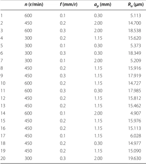
To establish a regression model of the surface roughness, a bar with a diameter of 66.5 mm was selected as the test object according to the actual experiment conditions. The central composite design can fit the response surface bet-ter than the Box–Benhnken design. At the same time, it is advisable that the experiment level not exceed the bound-ary of the cube to avoid exceeding the processing capacity of the machine. To reduce the number of experiments and ensure the accuracy of the results, the central composite inscribed design method was selected. The value of α was set to ± 1. Table 2 shows the experiment design and results.
As mentioned above, to ensure the comprehensiveness of the parameter optimization and the comparability of the results, a task-based parameter optimization method was chosen. The designated processing task is to process a bar with a diameter of 90–84 mm, the cutting length is equal to 30 mm. In addition, it is assumed that the machine starts to perform a fast forward after 30 s of a standby period.
To establish a multi-objective optimization equation, the following parameters or data need to be measured and acquired.
According to the actual measurement of SMTCL CAK50135di, the stand-by power under the selected cut-ting parameter is 321 W. The tool used is produced by Zhuzhou Cemented Carbide Cutting Tools Co., Ltd. The cutting tool material is YT15 and its weight is 474 g.
The cutting fluid needs regular supplementation and replacement, and according to an investigation on machine tools, the coolant is water-based, the specifica-tions of the cutting fluid is 20 L/barrel, the ratio of oil to water is 1:10, and the frequency of replacement is 5 months. The machine tool runs 22 days per month, with coolant applied for 8 h per day. The remaining coolant to be replaced is approximately 8 L.
The carbon emission factors used are as shown in Table 3.
4.2 Establishment of Multi‑Objective Optimization Model The experiment data recorded in Table 2 can be regressed using a response surface method, see Appendix A for details, and the surface roughness model is therefore as follows:
Applying the above data, combined with Section 3, the multi-objective optimization equations for machining tasks is obtained, and at the same time, the restrictive conditions are given according to the actual situation.
(15)
Ra= −11.556+203.16f −343.4f2.
Figure 4 Experiment setup
Table 2 Design of regression analysis experiment n (r/min) f (mm/r) ap (mm) Ra (μm)
1 600 0.1 0.30 5.113
2 450 0.2 2.00 14.700
3 600 0.3 2.00 18.538
4 300 0.2 1.15 15.620
5 300 0.1 0.30 5.373
6 300 0.3 0.30 18.349
7 300 0.1 2.00 5.209
8 450 0.2 1.15 15.916
9 450 0.3 1.15 17.919
10 600 0.2 1.15 14.727
11 600 0.3 0.30 17.985
12 450 0.2 1.15 15.812
13 450 0.2 1.15 15.462
14 600 0.1 2.00 4.907
15 450 0.2 1.15 15.976
16 450 0.2 1.15 15.113
17 450 0.1 1.15 6.028
18 450 0.2 0.30 14.977
19 450 0.2 1.15 15.090
20 300 0.3 2.00 19.630
Table 3 Equivalent carbon emission factors
Name of carbon emission factors Quantitative value
CFene (g-CO2/kW·h) 724.2
CFtool (g-CO2/kg) 29600
CFc_pro (g-CO2/L) 2850
CFc_dis (g-CO2/L) 4000
CFmaterial (g-CO2/kg) 2690
where
where Δ is a corrected coefficient, of which any value greater than the cutting depth will be reasonable.
5 Results and Discussion 5.1 Analysis of Optimization Results
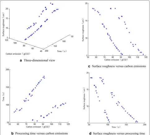
A non-dominated sorting genetic algorithm with an elitist strategy (NSGA-II) is one of the most popular multi-objec-tive genetic algorithms, which reduces the complexity of the non-inferior sorting genetic algorithm and has the advantages of a fast running speed and good convergence of the solution set [30]. In this paper, NSGA-II is employed as a computing tool for the Pareto frontier in multi-objective optimization. The population size is 50 and the reproductive algebra is set to 2000, with the remaining parameters set by default. Matlab R2014a is used to sim-ulate the optimization model, and the Pareto front of the multi-objective optimization is as shown in Figure 5. The corresponding Pareto frontier is shown in Appendix C.
The curve in Figure 5(a) reflects the trade-off among the three objectives. Meanwhile, the relationships
(16) min
C=724.2×Eene+Ttooltcut ×CFtool×Mtool+ (tcut+tidle)3168 ×89,
t=tcut +tidle,
Ra= −11.556+203.16f −343.4f2,
(17) s.t.,
300≤n≤600, 0.1≤f ≤0.3, 0.3≤ap≤2,
(18) Eene=
321.4×30+
750.9+115.4×n/60+11.32×(n/60)2 ×tidle
3.6×10⁶
+
750.9+115.4×n/60+11.32×(n/60)2+2.256×πd·n/60·f ·ap
×tcut−1
3.6×10⁶
+
750.9+115.4×n/60+11.32×(n/60)2+2.256×πd·n/60·f ·rem
R−r,ap
×tcut−2
3.6×10⁶ ,
(19)
tidle = 498
19 +ceil
R−r ap
×
8 n/60·f +
228 190
,
tcut =tcut−1+tcut−2,
tcut−1=floor
R−r ap
× 30
n/60·f,
tcut−2=ceil
rem
R−r,ap
/�
× 30
n/60·f,
Ttool = 60 f
6×10⁵ 3.1415926×n/60
2.13
,
between the two targets among the three goals are shown in Figure 5(b), (c), and (d). From Figure 5(b), there is an approximate linear relationship between the processing time and carbon emissions. That is, within the bound-ary of the system, the increase in the processing time will
cause an approximately linear increase in carbon emis-sions, which has a certain relationship with the selec-tion of the system boundaries, but little effect on the law. From Figure 5(c), the amount of carbon emissions and surface roughness are inversely proportional. This means that reducing the surface roughness often results in greater carbon emissions. The same relationship is also shown between the surface roughness and the processing time (Figure 5(d)).
The cutting parameters for minimizing the carbon emissions are ap= 1.5 mm, n= 300 r/min, and f= 0.3
mm/r, with 55.57 g of carbon emissions, a processing time of 79.28 s, and a surface roughness of 18.49 μm. The parameters minimizing the processing time are ap= 1.5
mm, n= 600 r/min, and f= 0.3 mm/r, with carbon emis-sions of 83.07 g, a processing time of 53.94 s, and a sur-face roughness of 18.49 μm. Usually, the bigger the cutting parameters are, the smaller the processing time; however, the cutting depth here is not the maximum in the optional interval because the processing task-based optimization model was chosen in this study. When the specified total processing depth is 3 mm, for the maxi-mum spindle speed and feed rate, the total processing time of the cutting depth in the interval [1.5, 2.0] is the same, which is the least used. Here ap= 1.5 mm is given
When one of them reaches the minimum, the other two goals are often unsatisfactory.
In general, the Pareto solution set obtained by the multi-objective optimization problem is at the same non-dominated solution level, and there are many solutions with the same degree of congestion, and the dimensions of each optimization target are often different. There is no unified standard, making a comparison difficult, which causes problems for decision makers. Usually, the execution solution is selected from the Pareto frontier based only on subjective consciousness or personal expe-rience. To this end, this study adopts the TOPSIS method to sort the three targets.
In this research, the TOPSIS method is applied to rank the Pareto frontier. TOPSIS is one of the commonly used multi-attribute decision-making methods. The idea is to sort the finite objects to be evaluated based on the ideal optimal and worst values using the Euclidean distance, obtaining the degree of approximation of each point with these values, and thus giving the optimal solution. See Appendix C for the Pareto frontier results. Accord-ing to the calculation, the optimal approximation is 0.6206, and the corresponding decision variables are
ap= 1.88 mm, n= 560 r/min, and f= 0.12 mm/r. Carbon
emissions under the decision variables are 104.94 g·CO2,
the processing time is 97.59 s, and the surface roughness is 7.65 μm.
5.2 Analysis of the Main Effect Factors
To analyze the impact of the decision variables on each goal, the response values of the carbon emissions and processing time are calculated according to Table 4, and an S/N ratio analysis is carried out. The S/N ratio is uti-lized to measure how the response changes relative to the nominal/target values. For static designs, Minitab offers four signal-to-noise ratios. The purpose of multi-objec-tive optimization in this study is to minimize the car-bon emissions, processing time, and surface roughness. Thus, the lower-the-better type of objective function was selected [31]. The conversion relation between the S/N ratio and the signal is as follows:
where n is the number of experiments, and yi is the value of the carbon emissions or processing time.
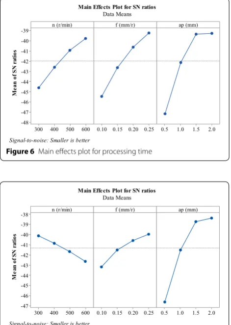
The S/N ratio at each level for the various factors of the carbon emissions and processing times is plotted in Fig-ures 6 and 7 respectively. As shown in Figure 6, on the whole, the larger the cutting parameters are, the smaller the processing time. The condition at ap= 1.5 mm or
2.0 mm, n= 600 r/min, and f= 0.25 mm/r can be consid-ered as the level at which the processing time is minimal within the given range of parameters. This is because this study adopted a task-based optimization model, under which the spindle speed and feed rate are fixed, and for a cutting depth of 3 mm, when ap= 1.5 mm or 2.0 mm, two
cutting processes are needed, and therefore the process-ing times under these two sets of cuttprocess-ing parameters are the same. In fact, the machining processing time is the same when the cutting depth is located within the inter-val [1.5 mm, 2 mm).
In addition, the carbon emissions will be at minimum when ap= 2.0 mm, n= 300 r/min, and f= 0.25 mm/r
within the given range of parameters. From the results, it can be found that, within the selected cutting param-eters, the cutting parameters that minimize the carbon
(20) S
N = −10×lg
1
n n
i=1
y2i
,
emissions differ from those that minimize the process-ing time, even the law of change is reversed (the spindle speed has the opposite effect on the carbon emissions and processing time). However, whether it is for the carbon emissions or processing time, the optimal result depends on the selected cutting parameters. The selec-tion of the cutting parameter values directly determines the accuracy of the optimization results. This means that the optimal values of this part are only optimal among the selected discrete cutting parameters and are not glob-ally optimal.
Tables 5 and 6 are the S/N ratios of the carbon emis-sions and processing time, respectively. A first rank con-tribution is assigned to the highest range value. For both the carbon emissions and processing time, the cutting depth is the most significant factor, followed by the feed rate, and the spindle speed is the least significant factor.
5.3 Coupling Effect Analysis
The effect of the cutting parameters on the carbon emis-sions and processing time based on the processing task in this study can be observed from the contour plots in
Table 4 Levels and factors selected for S/N ratios
Spindle speed
(r/min) Feed rate (mm/r) Cutting depth (mm)
1 300 0.1 0.5
2 400 0.15 1
3 500 0.2 1.5
4 600 0.25 2
600 500 400 300 -39 -40 -41 -42 -43 -44 -45 -46 -47 -48
0.25 0.20 0.15
0.10 0.5 1.0 1.5 2.0 n (r/min)
Me
an
of
SN
ra
tios
f (mm/r) ap (mm) Main Effects Plot for SN ratios
Data Means
Signal-to-noise: Smaller is better
Figure 6 Main effects plot for processing time
600 500 400 300 -38 -39 -40 -41 -42 -43 -44 -45 -46 -47
0.25 0.20 0.15
0.10 0.5 1.0 1.5 2.0 n (r/min)
Me
an
of
SN
ra
tios
f (mm/r) ap (mm) Main Effects Plot for SN ratios
Data Means
Signal-to-noise: Smaller is better
Figures 8 and 9. For the processing time during the turn-ing process, in general, the greater the values of the cut-ting parameters are, the shorter the processing time, although the influence rate of the decision variables on the processing time is different. The effect of the cutting depth on the processing time is more significant than that of the spindle speed on the processing time based on the contour map (Figure 8(a)). The effect of the cutting depth on the processing time is more significant than that of the feed rate on the processing time (Figure 8(b)). The effect of the feed rate on the processing time is more significant than that of the spindle speed (Figure 8(c)). The influence of the cutting depth, feed rate, and spindle speed on the processing time is gradually weakened. This is consistent with the analysis results in Section 5.2. Thus, the mini-mum processing time can be achieved when the levels of the spindle speed, feed rate, and cutting depth are at their highest levels.
The value of the carbon emissions is minimized when the cutting depth and the feed rate were at their high-est values, and the spindle speed was at its lowhigh-est value (Figure 9). Moreover, as stated in the graphs, the effects
Table 5 S/N ratios of carbon emissions
Level ap n f
1 − 46.62 − 40.11 − 43.16
2 − 41.52 − 40.83 − 41.51
3 − 38.72 − 41.66 − 40.58
4 − 38.37 − 42.63 − 39.97
Delta 8.25 2.52 3.19
Rank 1 3 2
Table 6 S/N ratios of processing time
Level ap n f
1 − 47.17 − 44.6 − 45.45
2 − 42.14 − 42.62 − 42.64
3 − 39.34 − 40.94 − 40.61
4 − 39.27 − 39.76 − 39.22
Delta 7.89 4.84 6.23
Rank 1 3 2
a
b
c
f (mm/ r)*n (r/ min)
600 500
400 300
0.28
0.24
0.20
0.16
0.12
ap (mm)*n (r/ min)
600 500
400 300
2.0
1.5
1.0
0.5
ap (mm)*f (mm/ r)
0.28 0.24 0.20 0.16 0.12 2.0
1.5
1.0
0.5 n (r/ min) 450
f (mm/ r) 0.2 ap (mm) 1.15 Hold Values
> – – – – < 100 100 200 200 300 300 400 400 500 500 Time (s)
Figure 8 Contour plots of processing time
f (mm/ r)*n (r/ min)
600 500
400 300
0.28
0.24
0.20
0.16
0.12
ap (mm)*n (r/ min)
600 500
400 300
2.0
1.5
1.0
0.5
ap (mm)*f (mm/ r)
0.28 0.24 0.20 0.16 0.12 2.0
1.5
1.0
0.5 n (r/ min) 450f (mm/ r) 0.2 ap (mm) 1.15 Hold Values
> – – – < 100 100 200 200 300 300 400 400 (gCO2) Carbon
a
b
c
of the cutting depth on the carbon emissions are more significant than those of the spindle speed on the carbon emission (Figure 9(a)), whereas the effects of the cutting depth on the carbon emissions are more significant than the feed rate on the carbon emissions (Figure 9(b)), This is also consistent with the analysis results in Section 5.2.
5.4 Sensitivity Analysis
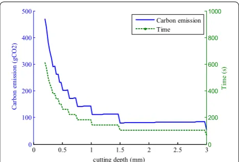
To further analyze the changing rules of the target to be evaluated with the decision variables, a sensitivity analy-sis method is adopted (Figures 10, 11, 12). From the per-spective of the target to be evaluated, it is easy to find that the processing time decreases monotonously with the increase in the three decision variables. The carbon emis-sions decreased monotonously with an increase in the feed rate and the cutting depth; however, with an increase in the spindle speed, the carbon emissions show a decreas-ing trend first, followed by an increasdecreas-ing trend. From the impact of the decision variables on the evaluation objec-tives, the objectives to be optimized vary smoothly with the
spindle speed and feed rate, but with an increase in the cut-ting depth, they show a stepped decrease. This is because, in this study, a processing task-based optimization model was selected, and for the processing depth (3 mm) speci-fied in this paper, a cutting depth that can be divided by 3 without any remainder (e.g., 0.5 mm, 0.75 mm, 1.0 mm, 1.5 mm) is a watershed for the processing time and car-bon emissions. Between the two watersheds, although the cutting depth changes, the total processing time remains unchanged. However, the processing time at the watershed will decline in a cliff-like descent. This is because, at the watershed, the cutting cycle processing times will change suddenly, which will lead to the step change in the process-ing time. The step change of the processprocess-ing time directly affects the step change of the carbon emissions. However, there is a weak upward trend in carbon emissions between the two watersheds, the reason for which is as follows: although the processing times between the two watersheds are constant, that is, the idle time and cutting time remain unchanged, with the increase in the cutting depth, the devi-ation between the setting of the cutting depth and the cut-ting depth during the last cutcut-ting increases, which causes an increase in the cutting power fluctuation of the machine tool, leading to an increase in the energy consumption during the entire processing process, naturally causing an increase in the carbon emissions.
6 Conclusions
In this study, a task-based multi-objective optimization model that incorporates the environment impact, prod-uct quality, and processing efficiency was considered, and the following conclusions were obtained.
1. Different optimal cutting parameters were obtained for different optimization purposes. When only the processing time is optimized, the cutting parameters
200 300 400 500 600
120 130 140 150 160 170 180 190
Spindle speed (r/min)
Car
bon
em
issi
on
(g
CO
2)
100 150 200 250 300 350 400 450
Ti
me
(s
)
Carbon emission Time
Figure 10 Influence of spindle speed on the optimization target
0 0.05 0.1 0.15 0.2 0.25 0.3 0.35
0 200 400 600
Feed rate (mm/r)
Ca
rb
on
em
issi
on
(g
CO
2)
0 500 1000 1500
Ti
me
(s
)
Carbon emission Time
Figure 11 Influence of feed rate on the optimization target
0 0.5 1 1.5 2 2.5 3
0 100 200 300 400 500
cutting depth (mm)
Car
bon
em
issi
on
(g
CO
2)
0 200 400 600 800 1000
Ti
me
(s
)
Carbon emission Time
selected should be as large as possible. When only the surface roughness is optimized, a smaller feed rate should be selected. When only carbon emissions are optimized, the cutting parameters need to be considered comprehensively, as is the case when the three targets are simultaneously optimized.
2. The cutting depth among the other parameters has the most significant effect on both the carbon emis-sions and processing time, and the spindle speed has the least significant effect by comparison, with the feed rate being between them.
3. The variation of the carbon emissions and processing time with the decision variables is analyzed. The rea-son for the decrease in carbon emissions and time in a cliff-like descent is analyzed emphatically. This also explains the reason for the slight increase in carbon emissions between the two watersheds.
4. Future studies will be conducted on milling, grinding, drilling, and other extensions. Meanwhile, factors such as the cutting tools and machining operations will be added to the decision variables, and the deci-sion variables will be optimized to find the trade-off that takes the environment impact, product quality, processing efficiency, and even cost into account.
Abbreviations
A: a constant denoting the coefficient related to the operation conditions; ap: the depth of the cut (mm); C: total carbon emissions in metal cutting
processes (g); Cconsum: consumable carbon emissions (g); Cair: carbon emissions
for preparing compressed air (g); Cchips: carbon emissions from chips (g); Ccool:
carbon emissions from the use of coolant (g); Ccool-w: carbon emissions from
waste coolant (g); CFc-pro: carbon emission factor of coolant fluid production
(g-CO2/L); CFc-dis: carbon emission factor for waste coolant disposal (g-CO2/L); CFdisposal: carbon emission factor for chips disposal (g-CO2/kg); CFene: carbon
emission factor of electricity (g/kwh); CFmaterial: carbon emission factor of
material production (g-CO2/kg); CFtool: carbon emission factor of cutting tools
(g-CO2/g); Cresource: carbon emission caused by resource depletion (g); Ctrans:
transferable (transitional) carbon emissions (g); Ctool: carbon emissions caused
by tools, which include tool usage stage and tool sharpening process (g); C tool-w: carbon emissions from scrap tool treatment (g); Cwaste: carbon emissions
caused by waste generation (g); Eene: energy consumption of machine tools
(kW·h); f: feed rate (mm/r); h: spindle speed, feed rate, and depth of cut; Mtool:
weight of a tool (g); n: spindle speed (r/min); Ra: roughness height; t: the sum
of tidle and tcut(s); tchan: tool changing processing time (s); tcut: the actual cutting
processing time (s); tclam: Workpiece clamping processing time (s); tstand-by: the
period when the machine tool stays without any operations (s); tidle: the period
when the spindle rotates without cutting (s); tset: tool setting processing time
(s); tpro: programming time (ignored during mass processing) (s); tunl:
unload-ing blank processunload-ing time (s); Ttool: life cycle of cutting tools (min); x, y, z, m:
influence index; β: the coefficients of each term; ε: residual error.
Authors’ Contributions
YL and DG were in charge of the whole trial; ZJ wrote the manuscript; XL assisted with sampling and laboratory analyses. All authors read and approved the final manuscript.
Authors’ Information
Zhipeng Jiang, born in 1988, is currently a PhD candidate at Harbin Institute of Technology, China. His research interests include green manufacturing and mechatronics engineering.
Dong Gao, born in 1970, is currently an professor at Harbin Institute of Tech-nology, China. He received his PhD degree from Harbin Institute of TechTech-nology, China, in 1999. His research interests include sustainable manufacturing tech-niques and error modeling and compensation for heavy-duty machine tool.
Yong Lu, born in 1971, is currently an professor at Harbin Institute of Tech-nology, China. He received his PhD degree from Harbin Institute of TechTech-nology, China, in 2000. His research interests include space on-orbit service technol-ogy and intelligent tool condition monitoring technoltechnol-ogy.
Xianli Liu, born in 1961, is currently an professor at Harbin University of Science & Technology, China. His research interests include high efficiency machining and cutting tool technology.
Competing interests
The authors declare that they have no competing interests.
Funding
Supported by National Hi-tech Research and Development Program of China (863 Program, Grant No. 2014AA041503), and National Natural Science Foun-dation of China (Key Program, Grant No. 51235003).
Author Details
1 School of Mechatronics Engineering, Harbin Institute of Technology, Har-bin 150001, China. 2 State Engineering Laboratory of High Efficiency Cutting and Tool, Harbin University of Science and Technology, Harbin 150080, China.
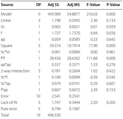
Appendix A. Response Surface Analysis
Minitab was used to analyze the response surface experi-ment, and a variance analysis, model summary, and regression model of the surface roughness were obtained.
The regression equation in uncoded units space is as follows:
1. Considering the total effect in Table 7, in this case, the P value of the regression term is 0.000, which indicates that the original hypothesis should be rejected and that the model is generally valid. Mean-while, the P value of a lack-of-fit is 0.203, which is significantly higher than the significant level of 0.05. Accepting the original hypothesis, it is considered that there is no unfit phenomenon in this model. 2. Considering the total effect of the fit, in this case,
R-Sq is close to R-Sq(adj), and the fitting effect of the model is considered good. Here, R-Sq (pred) is closer to the R-Sq value, which is larger, indicating that the future prediction using this model is reliable (Table 8).
3. Considering the significance of each effect, it can be seen from the table that the corresponding probabil-ity values of feed rate f and its squared term are less than 0.05, indicating that these effects are significant. The probability values corresponding to the other items are far greater than 0.05, which is obviously greater than the significant level. It is considered that these items are not significant.
(21) Ra= −10.99+0.0049Vc+194f +0.95ap
Based on the above analysis, we know that, except for feed rate f and its squared term, the other items are not significant and should be eliminated, and thus we need to re-fit the new model.
Regression equation in uncoded units,
1. The P value of the regression term is 0.000 (Table 9), which indicates that the original hypothesis should be rejected and that the model is generally valid. Meanwhile, the P value of a lack-of-fit is 0.219, which is significantly higher than the significant level of 0.05. Accepting the original hypothesis, it is consid-ered that there is no unfit phenomenon even though seven items are deleted from the model.
2. Although there are seven fewer items in the model, R-Sq is close to R-Sq(adj), and the fitting effect of the model is considered good. R-Sq (pred) is closer to the R-Sq value, which is larger, indicating that the future prediction using this model is reliable (Table 10).
(22) Ra= −11.556+203.16f −343.4f2.
3. It can be seen from the table that the corresponding probability values of feed rate f and its squared term
are less than 0.05, indicating that these two effects are significant. This shows that the effect of the regres-sion is still good after deleting the insignificant inter-action.
Appendix B. Processing Time Calculation
As the requirement of the experiment mentioned above, a bar with a diameter of 90 mm is required to be machined to a diameter of 84 mm, that is, the total cutting depth on one side is 3.0 mm. When the cutting depth is set at 0.5, 1.0, 1.5, and 2.0 mm, the cycle is six, three, two, and two processing times, respectively. For a 2.0 mm cutting depth, two cycles are needed, one for a cutting depth of 2.0 mm, and the other for a cutting depth of 1.0 mm instead of 2.0 mm. Then, the fourth set of experimental parameters in Table 3 were taken as an example calculation.
During the experiment, the tool path (fast forward, feed, and withdraw) and the distance were as shown in Figure 2, with Lx1=200 , Lz1=400 , Lz2=2 , Lz3=30 , and Lx2=6 . The standby processing time of each group is set at a fixed value of 30 s, and combined with the information of the machine tool coordinate system set-tings, the idle running processing time will be as follows:
Table 7 Analysis of variance
Source DF Adj SS Adj MS F‑Value P‑Value
Model 9 493.989 54.8877 216.03 0.000
Linear 3 1.798 0.5992 2.36 0.133
Vc 1 0.002 0.0021 0.01 0.929
f 1 1.737 1.7370 6.84 0.026
ap 1 0.059 0.0585 0.23 0.642
Square 3 59.374 19.7914 77.90 0.000
Vc*Vc 1 0.001 0.0006 0.00 0.961
f*f 1 28.426 28.4262 111.88 0.000
ap*ap 1 0.337 0.3371 1.33 0.276
2-way interaction 3 0.781 0.2604 1.02 0.422
Vc*f 1 0.100 0.0999 0.39 0.545
Vc*ap 1 0.074 0.0741 0.29 0.601
f*ap 1 0.607 0.6072 2.39 0.153
Error 10 2.541 0.2541
Lack-of-fit 5 1.747 0.3494 2.20 0.203
Pure error 5 0.794 0.1587
Total 19 496.530
Table 8 Model summary
S R‑sq (%) R‑sq (adj) (%) R‑sq (pred) (%)
0.504053 99.49 99.03 97.21
Table 9 Analysis of variance
Source DF Adj SS Adj MS F‑Value P‑Value
Model 2 491.814 245.907 886.47 0.000
Linear 1 432.846 432.846 1560.36 0.000
f 1 432.846 432.846 1560.36 0.000
Square 1 58.969 58.969 212.58 0.000
f*f 1 58.969 58.969 212.58 0.000
Error 17 4.716 0.277
Lack-of-fit 12 3.922 0.327 2.06 0.219
Pure error 5 0.794 0.159
Total 19 496.530
Table 10 Model summary
S R‑sq (%) R‑sq (adj) (%) R‑sq (pred) (%)
Although the cutting depth is set to a certain value, the total depth to be cut is not necessarily an integral multi-ple of the cutting depth. When the cutting depth is dif-ferent from the set cutting depth in the last cutting, the cutting power of the machine tool will change. Therefore, this study calculated the processing time with the same cutting depth as the set cutting depth, and the process-ing time with a different cuttprocess-ing depth as the set cuttprocess-ing depth, which were called tcut−1 and tcut−2 , respectively. When the total depth to be machined is an integer multi-ple of the set cutting depth, tcut−2=0.
Appendix C. Carbon Emission Calculation Carbon Emissions from Consumable Carbon Emissions Combined with the power calculation formula of the machine tools, the carbon emissions from the consum-able carbon emissions is as follows:
Carbon Emissions from Cutting Tools
The carbon emissions from the cutting tools includes carbon emissions from the tool production and from tool re-sharpening after a tool failure. The tool
(23) tidle =
400
1900/60+ceil
3
ap
×
8
n/60·f +
38
1900/60
+ 430
1900/60
= 498
19 +ceil
3
ap
× 480
n·f +
228
190
.
(24) tcut =tcut−1+tcut−2,
tcut−1=floor
R−r ap
× 30
n/60·f,
tcut−2=ceil
rem
R−r,ap
/�
× 30
n/60·f.
(25) Eene=
321.4×30+
750.9+115.4×n/60+11.32×(n/60)2
×tidle
3.6×10⁶
+
750.9+115.4×n/60+11.32×(n/60)2+2.256×πd·n/60·f ·ap
×tcut−1
3.6×10⁶
+
750.9+115.4×n/60+11.32×(n/60)2+2.256×πd·n/60·f ·rem
R−r,ap
×tcut−2
3.6×10⁶ ,
(26) Cconsum=724.2×Eene.
re-sharpening process is not included in this case owing to limited conditions. The tool quality is 474 g, and therefore, the carbon emissions caused by tool wear can be obtained.
The calculating method of the tool life is shown in the following formula. According to the cutting parameters, the calculating method of the tool life is obtained [25]:
Carbon Emissions from Coolant Fluid
Thus, carbon emissions caused by coolant can be calcu-lated based on Section 4.1.
Thus, the formula for calculating the carbon emissions is as follows:
(27) Ctool =
tcut Ttool
×29.6×474.
(28) Ttool =
60
f
6×10⁵ 3.1415926×n/60
2.13
.
(29)
Ccool=
(tcut+tidle)
5×22×8×60×60(2850×20+4000×8)
= (tcut+tidle)
3168 ×89.
(30) C=724.2×Eene+ tcut
Ttool
×14030.4+(tcut+tidle)
3168 ×89.
Appendix D. Pareto Front Solution Set
Table 11 Pareto front solution set
No. Cutting depth (mm)
Spindle speed (r/min)
Feed rate (mm) Carbon emissions (g‑CO2)
Processing
time (s) Surface roughness (μm)
Relative closeness Note
1 1.50 300 0.30 55.57 79.28 18.49 0.5007 Minimum carbon emission
2 1.50 300 0.10 91.26 180.61 5.33 0.4943 Minimum surface roughness
3 1.50 300 0.10 91.26 180.61 5.33 0.4943 Minimum surface roughness
4 1.50 600 0.30 83.07 53.94 18.49 0.5029 Minimum processing time
5 1.93 600 0.10 116.97 104.61 5.33 0.6056 Minimum surface roughness
6 1.51 546 0.30 77.39 56.48 18.49 0.5073
7 1.99 600 0.19 94.31 68.83 14.57 0.5378
8 1.66 335 0.22 64.48 89.43 16.70 0.5000
9 1.52 300 0.13 78.50 144.21 9.22 0.5175
10 1.53 300 0.26 58.61 87.56 17.99 0.4885
11 1.53 333 0.25 61.72 84.31 17.64 0.4965
12 1.89 560 0.13 101.99 92.52 8.76 0.6187
13 1.53 336 0.24 62.74 85.92 17.31 0.4979
14 1.55 300 0.15 74.01 131.14 11.02 0.5172
15 1.52 326 0.15 75.68 124.45 10.80 0.5407
16 1.98 559 0.20 87.94 68.55 15.61 0.5259
17 1.61 300 0.28 57.08 82.42 18.43 0.4934
18 1.54 300 0.11 86.51 166.75 6.64 0.5042
19 1.52 300 0.12 83.44 158.22 7.55 0.5102
20 1.57 310 0.18 68.07 109.66 13.99 0.5093
21 1.50 300 0.10 90.22 177.63 5.59 0.4966
22 1.55 300 0.18 67.41 112.31 14.01 0.5026
23 1.55 301 0.14 76.72 138.38 9.94 0.5193
24 1.53 300 0.11 87.92 170.81 6.24 0.5012
25 1.89 590 0.11 110.87 98.26 6.77 0.6162
26 1.59 314 0.17 69.44 111.70 13.46 0.5154
27 1.94 599 0.10 114.82 101.59 5.91 0.6102
28 1.88 560 0.12 104.94 97.59 7.65 0.6206 Minimum overall
29 1.51 309 0.10 91.55 176.00 5.33 0.5021 Minimum surface roughness
30 1.91 567 0.12 104.45 94.49 8.13 0.6199
31 1.52 300 0.11 84.60 161.31 7.19 0.5084
32 1.98 594 0.12 107.61 91.45 8.14 0.6165
33 1.55 301 0.13 77.70 141.14 9.57 0.5189
34 1.95 600 0.21 91.19 64.18 16.18 0.5153
35 1.77 600 0.17 96.91 74.07 12.81 0.5677
36 1.98 596 0.21 90.75 64.28 16.22 0.5150
37 1.72 300 0.17 69.77 117.41 13.16 0.5063
38 1.51 300 0.11 85.11 163.05 7.02 0.5071
39 1.71 327 0.17 72.28 112.90 12.66 0.5288
40 1.95 600 0.15 100.03 78.02 11.57 0.5851
41 1.50 544 0.29 77.71 57.56 18.48 0.5051
42 1.96 558 0.21 87.39 67.91 15.83 0.5231
43 1.92 600 0.10 116.92 104.61 5.33 0.6057 Minimum surface roughness
44 2.00 599 0.18 95.29 70.59 13.99 0.5469
45 1.55 301 0.12 82.24 153.67 7.99 0.5140
46 1.89 589 0.11 111.72 99.91 6.46 0.6149
47 1.54 304 0.13 80.70 148.25 8.52 0.5190
Received: 26 March 2019 Revised: 10 July 2019 Accepted: 4 November 2019
References
[1] Ministry of Ecology and Environment of the People’s Republic of China. China Vehicle Environmental Management Annual Report (2018). http:// www.vecc-mep.org.cn/huanb ao/conte nt/944.html. (in Chinese) [2] X L Liu, Z P Jiang, M Y LI, et al. New rounded end mill for mold processing
based on scallop-height. Journal of Mechanical Engineering, 2015, 51(5): 192-204. (in Chinese)
[3] D F Liu, X J Zhang. The influence of hard turning technology on product quality and cost. Die and Mould Technology, 2006, 5(6): 57-60. (in Chinese) [4] https ://unfcc c.int/proce ss-and-meeti ngs/the-kyoto -proto
col/what-is-the-kyoto -proto col/what-is-col/what-is-the-kyoto -proto col /(accessed on 24 May 2019).
[5] R Huang, M Riddle, D Graziano, et al. Energy and emissions saving poten-tial of additive manufacturing: The case of lightweight aircraft compo-nents. Journal of Cleaner Production, 2016, 135: 1559-1570.
[6] R Li, Q Zhang, X Zhang, et al. Control method for steel strip roughness in Two-stand temper mill rolling. Chinese Journal of Mechanical Engineering, 2015, 28(3): 573-579.
[7] D B Tang, M Dai. Energy-efficient approach to minimizing the energy consumption in an extended job-shop scheduling problem. Chinese Journal of Mechanical Engineering, 2015, 28(5): 1048-1055.
[8] G Campatelli, L Lorenzini, A Scippa. Optimization of process parameters using a Response Surface Method for minimizing power consumption in the milling of carbon steel. Journal of Cleaner Production, 2014, 66(2): 309-316.
[9] J Wójcicki, M Leonesio, G Bianchi, et al. Integrated energy analysis of cutting process and spindle subsystem in a turning machine. Journal of Cleaner Production, 2018, 170: 1459-1472.
[10] Q Zhong, R Tang, T Peng. Decision rules for energy consumption mini-mization during material removal process in turning. Journal of Cleaner Production, 2016, 140: 1819-1827.
[11] P S Bilga, S Singh, R Kumar. Optimization of energy consumption response parameters for turning operation using Taguchi method. Jour-nal of Cleaner Production, 2016, 137: 1406-1417.
[12] B Wang, Z Liu, Q Song, et al. Proper selection of cutting parameters and cutting tool angle to lower the specific cutting energy during high speed machining of 7050-T7451 aluminum alloy. Journal of Cleaner Production, 2016, 129: 292-304.
[13] Q Wang, F Liu, X Wang. Multi-objective optimization of cutting param-eters considering energy consumption. International Journal of Advanced Manufacturing Technology, 2014, 71(5-8): 1133-1142.
[14] Q Yi, C Li, Y Tang, et al. Multi-objective parameter optimization of CNC machining for low carbon manufacturing. Journal of Cleaner Production, 2015, 95: 256-264.
[15] Z J Liu, D P Sun, C X Lin, et al. Multi-objective optimization of the operat-ing conditions in a cuttoperat-ing process based on low carbon emission processing times. Journal of Cleaner Production, 2016, 124: 266-275.
[16] K He, R Tang, M Jin. Pareto fronts of cutting parameters for trade-off among energy consumption, cutting force and processing time. Interna-tional Journal of Production Economics, 2017, 185: 113-127.
[17] S A Bagaber, A R Yusoff. Multi-objective optimization of cutting param-eters to minimize power consumption in dry turning of stainless steel 316. Journal of Cleaner Production, 2017, 157: 30-46.
[18] W W Lin, D Y Yu, et al. Multi-objective teaching–learning-based optimiza-tion algorithm for reducing carbon emission and operaoptimiza-tion process-ing time in turnprocess-ing operations. Engineerprocess-ing Optimization, 2015, 47(7): 994-1007.
[19] C Camposeco-Negrete. Optimization of cutting parameters using Response Surface Method for minimizing energy consumption and maximizing cutting quality in turning of AISI 6061 T6 aluminum. Journal of Cleaner Production, 2015, 91: 109-117.
[20] W W Lin, D Y Yu, C Y Zhang, et al. Multi-objective optimization of machin-ing parameters in multi-pass turnmachin-ing operations for low-carbon manufac-turing. Proceedings of the Institution of Mechanical Engineers Part B Journal of Engineering Manufacture, 2017, 231(13): 2372-2383.
[21] Ic Yusuf Tansel, Saraloğlu Güler Ebru, Cabbaroğlu Ceren, et al. Optimisa-tion of cutting parameters for minimizing carbon emission and maximis-ing cuttmaximis-ing quality in turnmaximis-ing process. International Journal of Production Research, 2018, 56(11): 1-21.
[22] C Li, Q Xiao, Y Tang, et al. A method integrating Taguchi, RSM and MOPSO to CNC cutting parameters optimization for energy saving. Journal of Cleaner Production, 2016, 135: 263-275.
[23] Y Zhang, Q Liu, Y Zhou. Integrated optimization of cutting parameters and scheduling for reducing carbon emission. Journal of Cleaner Produc-tion, 2017, 53(5): 886-895.
[24] F Ma, H Zhang, H J Cao, Multi-objective cutting parameters optimiza-tion for low energy and minimum cutting fluid consumpoptimiza-tion. Journal of Mechanical Engineering, 2017, 53(11): 157-163. (in Chinese)
[25] C B Li . Multi-objective NC cutting parameters optimization model for high efficiency and low carbon. Journal of Mechanical Engineering, 2013, 49(9): 87-96. (in Chinese)
[26] Z P Jiang, D Gao, Y Lu, et al. Electrical energy consumption of CNC machine tools based on empirical modeling. The International Journal of Advanced Manufacturing Technology, 2018, https ://doi.org/10.1007/s0017 0-018-2808-x.
[27] Z H Zhou. Metal cutting theory. Shanghai Scientific and Technical Publish-ers, 1984. (in Chinese)
[28] S Kalpakjian, S R Schmid. Manufacturing engineering and technology: machining. Beijing: China Machine Press, 2006.
[29] E Oberg, F D Jones, H L Horton. Machinery’s Handbook. 26th ed. New York: Industrial Press Inc., 2000.
[30] K Deb, A Pratap, S Agarwal, et al. A fast and elitist multiobjective genetic algorithm: NSGA-II. IEEE Transactions on Evolutionary Computation, 2002, 6(2): 182-197.
[31] G Box. Signal-to-noise ratios, performance criteria, and transformations. Technometrics, 1988, 30(1): 1-17.
Table 11 (continued)
No. Cutting depth (mm)
Spindle speed (r/min)
Feed rate (mm) Carbon emissions (g‑CO2)
Processing
time (s) Surface roughness (μm)
Relative closeness Note
49 1.52 327 0.14 76.88 127.17 10.33 0.5428