Shielding properties of a conducting bar calculated with a boundary integral method

(1)

Advances in Radio Science, 3, 119–123, 2005 SRef-ID: 1684-9973/ars/2005-3-119

Advances in

Radio Science

Shielding properties of a conducting bar calculated with a boundary

integral method

L. O. Fichte, S. Lange, Th. Steinmetz, and M. Clemens

Professur für Theoretische Elektrotechnik und Numerische Feldberechnung, Helmut-Schmidt-Universität, Universität der Bundeswehr Hamburg, PO. Box 700822, 22008 Hamburg, Germany

Abstract. A plane rectangular bar of conducting and per-meable material is placed in an external low-frequency mag-netic field. The shielding properties of this object are in-vestigated by solving the given plane eddy current problem for the vector potential with the boundary integral equation method. The vector potential inside the rectangle is governed by Helmholtz’ equation, which in our case is solved by sep-aration. The solution is inserted into the remaining bound-ary integral equation for the exterior vector potential in the domain surrounding the bar. By expressing its logarithmic kernel as a Fourier integral the overall solution inside and outside the bar is calculated using analytical means only.

1 Introduction

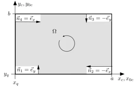
Subject of this investigation are the shielding properties of a rectangular bar of constant conductivityκi and permeabil-ity µi. The space outside the bar has the arbitrary con-stant permeabilityµa and conductivityκa=0. The vector rq=xqex+yqeyis pointing at the lower left corner of the bar, the dimensions of it beinga andb, as shown in Fig. 1. We name the cross-section of the barand its contourC=∂.

An exciting loop consists of two thin conductors, which carry the currentsi(t )and−i(t ), withi(t )=<{I ej ωt},I be-ing the phasor describbe-ing the complex current . They are located at

re= ±xeex.

The angular frequencyωis considered to be low enough so that displacement currents can be neglected:J∂

∂tD, where Jis the current density inside the bar andDthe electric flux. Thez-directed dimensions of both bar and loop are sup-posed to be infinite.

2 Differential equations for the vector potential

As all exciting currents are oscillating at one single fre-quency, all fields will show the same time dependency and can be expressed by their complex phasors.

Correspondence to: L. O. Fichte

([email protected])

Introducing a complex vector potential A as B=curlA, where B denotes the magnetic flux, and investigating its properties, we find that an additional term has to be added to the vector potential if we consider points inside the bar. The additional term can be expressed as the time domain in-tegral of the gradient of a complex electrical scalar potential φi(z)by

Z

(gradφi)dt =Cez,

where C denotes an unknown complex constant. The vec-tor potentialAiinside the bar can be redefined by using the Buchholz convention

A∗_i =Ai +

Z

grad8idt=Ai+Cez

from which the fields can be computed with Bi=curlA∗i and Ei= −j ωA∗i.

From Maxwell’s equations we find that the modified vec-tor potential inside the bar is governed by Helmholtz’ equa-tion, which for complex fields takes the form

1A∗_i −j ωµiκiA∗i =0. (1)

Outside the bar the equation

1Aa= −µaJe, (2)

is valid for the vector potentialAa. The exciting current den-sityJecan be expressed as

Je= {δ1(x−xe)−δ1(x+xe)}δ1(y)·Iez.

The symbol δ1(x−xo) denotes the one-dimensional Dirac function; accordingly, δ2 and δ3 are the two- and three-dimensional Dirac functions.

Since we allow onlyz-directed exciting currents, all vector potentials will also be exclusivelyz-directed. They can be described by theirz-componentsAaz andA∗_iz, respectively. The boundary conditions forAazandA∗_izare

Aaz=A∗iz−C ∧ 1

µano·gradAaz= 1

µino·gradA ∗ iz,

(2)

120 L. O. Fichte et al.: Shielding properties of a conducting bar calculated with a boundary integral method

SHIELDING PROPERTIES OF A CONDUCTING BAR

CALCULATED WITH A BOUNDARY INTEGRAL METHOD

Lars Ole Fichte, Sebastian Lange, Thorsten Steinmetz, Markus Clemens Professur f¨ur Theoretische Elektrotechnik und Numerische Feldberechnung

Helmut-Schmidt-Universit¨at Universit¨at der Bundeswehr Hamburg PO. Box 700822, D-22008 Hamburg, Germany Tel.(+49)40-6541 2460, Fax.(+49)40-6541 3764

ABSTRACT: A plane rectangular bar of con-ducting and permeable material is placed in an ex-ternal low-frequency magnetic field. The shielding properties of this object are investigated by solving the given plane eddy current problem for the vec-tor potential with the boundary integral equation method. The vector potential inside the rectangle is governed by Helmholtz’ equation, which in our case is solved by separation. The solution is inserted into the remaining boundary integral equation for the exterior vector potential in the domain surround-ing the bar. By expresssurround-ing its logarithmic kernel as a Fourier integral the overall solution inside and outside the bar is calculated using analytical means only.

1. INTRODUCTION

Subject of this investigation are the shielding prop-erties of a rectangular bar of constant conductivity

κi and permeability µi. The space outside the bar

has the arbitrary constant permeabilityµaand

con-ductivity κa = 0. The vector ~rq = xq~ex+yq~ey is

pointing at the lower left corner of the bar, the di-mensions of it beingaandb, as shown in Fig.1. We name the cross-section of the bar Ω and its contour

C=∂Ω.

An exciting loop consists of two thin conductors, which carry the currentsi(t) and−i(t), withi(t) =

<{Iejωt_}_, _I _{being the phasor describing the}

com-plex current . They are located at

~re =±xe~ex.

The angular frequency ω is considered to be low enough so that displacement currents can be ne-glected: J~¿ _∂t∂D~, where J~ is the current density inside the bar and D~ the electric flux.

Thez-directed dimensions of both bar and loop are supposed to be infinite.

2. DIFFERENTIAL EQUATIONS FOR THE VECTOR POTENTIAL

As all exciting currents are oscillating at one single PSfrag replacements

x, x0

y, y0

−I0 +I0

xc, x0c yc, y0c

a b

conducting bar

~rq

Figure 1: Screening bar and exciting loop

frequency, all fields will show the same time de-pendency and can be expressed by their complex phasors.

Introducing a complex vector potential A~ as B~ = curlA~, whereB~ denotes the magnetic flux, and in-vestigating its properties, we find that an additional term has to be added to the vector potential if we consider points inside the bar. The additional term can be expressed as the time domain integral of the gradient of a complex electrical scalar potential

ϕi(z) by w

(gradϕi)dt=C~ez,

where C denotes an unknown complex constant. The vector potential A~i inside the bar can be

re-defined by using the Buchholz convention

~

A∗i =A~i+

w

(gradϕi)dt=A~i+C,

from which the fields can be computed with

~

Bi= curlA~

∗

i and E~i =−jω ~A

∗

i.

From Maxwell’s equations we find that the modi-fied vector potentialinside the baris governed by

Fig. 1. Screening bar and exciting loop.

3 Derivation of Boundary Integral Equation (BIE)

In Green’s second theorem

Z Z

τ Z

(8 19−9 18)dτ=

= v

F=∂τ(8grad9

−9grad8)·nodF,

we insert the single component of the vector potentialAaas 9 and a kernel functionK satisfying1K=−δ3as8. As a result, we get an integral representation valid forAa: Aa= − v

F=∂τ(AagradK

−KgradAa)·nodF+

+µaI +∞ Z −∞ K xo=±xe yo=0

dzo.

The integrand of the surface integral at the right hand side of the above equation does not depend onz. Hence thez -directed integration is only affecting the kernel functionK, for which the elementary Kernel function

K= 1

4π r,

is inserted. Thereby we can define a new kernel functionG20 as

G20= +∞

Z

−∞

Kdzo=1 4π

+∞

Z

−∞

dzo p

(x−xo)2+(y−yo)2+(z−zo)2

= − 1 2π ln

p

(x−xo)2+(y−yo)2 ρo

!

= − 1 2π ln

_ρ

ρo

,

withρ=p(x−xo)2+(y−yo)2andρo=const. While we are aware that the above integral is divergent, it can be solved by performing a suitable renormalization.

The function G20 satisfies 1G20=−δ2, as is shown in Ehrich et al. (2000).

Helmholtz’ equation, which for complex fields takes the form

∆A~∗

i −jωµiκiA~

∗

i = 0. (1)

Outsidethe bar the equation

∆A~a=−µaJ~e, (2)

is valid for the vector potential A~a. The exciting

current densityJ~ecan be expressed as

~

Je={δ1(x−xe)−δ1(x+xe)}δ1(y)·I~ez.

The symbolδ1(x−xo) denotes the one-dimensional Dirac function; accordingly, δ2 andδ3are the

two-and three-dimensional Dirac functions.

Since we allow onlyz-directed exciting currents, all vector potentials will also be exclusivelyz-directed. They can be described by their z-componentsAaz

andA∗

iz, respectively. The boundary conditions for

AazandA∗izare

Aaz=A

∗

iz−C ∧

1

µa~no·gradA

az=

1

µi~no·gradA

∗

iz,

where~nois a unit vector normal to the boundary.

3. DERIVATION OF BOUNDARY INTE-GRAL EQUATION (BIE)

In Green’s second theorem

ww

τ

w

(Φ ∆Ψ−Ψ ∆Φ)dτ =

= {

F=∂τ

(Φ gradΨ−Ψ gradΦ)·~nodF,

we insert the single component of the vector po-tential Aa as Ψ and a kernel functionKsatisfying

∆K =−δ3 as Φ. As a result, we get an integral

representation valid forAa:

Aa=−

{

F=∂τ

(AagradK−KgradAa) ·~nodF+

+µaI

+w∞ −∞

K¯¯ ¯_x

o=±xe

yo=0

dzo.

The integrand of the surface integral at the right hand side of the above equation does not depend on z. Hence thez-directed integration is only affecting the kernel function K, for which the elementary Kernel function

K= 1 4πr,

PSfrag replacements

xc, x0c ~n1=~ey ~n2=−~ex

~n4=~ex ~n3=−~ey yc, y0c

Ω

a b

xq yq

Figure 2: Normals on boundary scetions

is inserted. Thereby we can define a new kernel functionG20as

G20= +w∞ −∞

Kdzo= 1 4π

+w∞ −∞

dzo p

(x−xo)2+ (y−yo)2+ (z−zo)2

= − 1

2πln( p

(x−xo)2+ (y−yo)2 ρo

) =−1

2πln( ρ ρo

),

withρ =p

(x−xo)2+ (y−yo)2 andρo = const. While we are aware that the above integral is di-vergent, it can be solved by performing a suitable renormalization.

The functionG20satisfies ∆G20=−δ2, as is shown

in [3].

If we use the new kernel and define the influence of the exciting loop as

Ae:=µaIG20|_x

o=±xe

yo=0

,

we can write the integral representation forAaas

Aa=−

z

C=∂Ω

(AagradG20−G20gradAa)·~nods+Ae.

We use the cross-section of the bar as integration domain Ω with its facet normals defined as shown in Fig. (2).

By taking into account the boundary conditions dis-cussed above, we get an integral representation for the vector potential outside the bar:

Aa=−

z

C=∂Ω

[(Wi−C) gradG20−

−G20

µa

µigradWi]·~nods+A

e.

(3) Fig. 2. Normals on boundary scetions.

If we use the new kernel and define the influence of the exciting loop as

Ae:=µaI G20|_x o=±xe yo=0

,

we can write the integral representation forAaas Aa= −

I

C=∂

(AagradG20−G20gradAa)· nods+Ae.

We use the cross-section of the bar as integration domain with its facet normals defined as shown in Fig. (2).

By taking into account the boundary conditions discussed above, we get an integral representation for the vector poten-tial outside the bar:

Aa= −

I

C=∂

[(A∗_i−C)gradG20−G20 µa µi

gradA∗_i] ·nods+Ae. (3)

It can be shown that

I

C=∂

(CgradG20)·nods=0,

so we can omit this term in Eq. (3).

In a last step we take the normal derivative ofAaon each of the four contour sections ofand move the observation point to the very same section, i.e.

(1)y =yq, (3)y =yq+b, (2)x =xq+a, (4)x =xq.

As a result, we get four independent integral equations µa

µi

n_o· gradA∗_i =n_o·grad (4)

 

 I

C=∂

(A∗_i gradG20−G20 µa

µi gradA ∗

i)nods+Ae

 



x=xq∨x=xq+a,y x,y=yq∨y=yq+b Conventionally, one would derive another boundary inte-gral equation, this one valid forA∗_i, using

G20i= 1 4jH

1 0(k

ρ ρ0

(3)

L. O. Fichte et al.: Shielding properties of a conducting bar calculated with a boundary integral method 121

PSfrag replacements

x/m y/m

−0.1 +0.1

~ B

Figure 3: Quadratic bar in homogenous field

Figure 4: Abs(A∗

i) for bar in homogenous field

As an additional verification, different values ofω, κ andµri= _µµ₀i are considered. We calculated the

av-erage of the absolute ofA∗

i over the cross-section of

the bar Ω as functions of . By this we can estimate which amount of the outside field permeates into the conducting area. The average ofA∗

i has been

normalized on the valueA0 = 1·10−6V s_A in Figs.

(5) and (6) and onA1= 1·10−7V s_A in Fig. (7).

4.2 SINGLE EXCITING LINE

In a next step, one conducting bar of quadratic cross-section with a = b = 0,1m is placed at ~rq= (−0.1,−0.1)m. One single exciting line, carry-ingI= 100 A, is placed at (0.0,−0.15) m, as shown in Figure (8).

Figure (9) displays the resulting lines of the mag-netic field forω= 501

s andκ= 57·10 6 A

Vm, µri= 1;

the field attenuation ∆Aa (and thereby the

shield-PSfrag replacements ¯_A/A

0

ω/(2π) / 1

s

Figure 5: ¯A/A0as a function ofω,κ, µconst.

PSfrag replacements ¯_A/A

0

κ/ 106 A Vm

Figure 6: ¯A/A0as a function ofκ,ω, µconst.

1

µri

Figure 7: ¯A/A0as a function ofµi,ω, κconst. Fig. 3. Quadratic bar in homogenous field.

PSfrag replacements

x/m y/m

−0.1 +0.1

~ B

Figure 4: Abs(A∗

As an additional verification, different values ofω, κ andµri=_µµi

0 are considered. We calculated the

i has been

normalized on the valueA0= 1·10−6V s_A in Figs.

s andκ= 57·10 6 A

Vm, µri= 1;

the field attenuation ∆Aa(and thereby the

0

ω/(2π) / 1

s

Figure 5: ¯A/A0as a function ofω,κ, µconst.

0

κ/ 106 A Vm

Figure 6: ¯A/A0as a function ofκ,ω, µconst.

1

µri

Figure 7: ¯A/A0as a function ofµi,ω, κconst.

Fig. 4. Abs(A∗_i) for bar in homogenous field.

as a kernel function Hanson and Yakovlev (2002). The func-tion H1₀ is the Hankel function of the first kind and order zero. The resulting system of two integral equations could be solved to yield the solutions for the two unknown func-tionsAaandA∗_i.

Here, we find a solution to Eq. (1) by separation, using a product of functions depending only on one coordinate for the descrition ofA∗_i.

A∗_i(xc, yc)= ∞

X

n=1

v1ncosh(βn(b−yc))+v3ncosh(βnyc)cos(αnxc)

+v2ncosh(βñ(a−xc))+v4n cosh(βñxc)cos(αñyc), αn=

nπ a , βn=

q α2

n+j ωκµ, ˜

αn= nπ

b , ˜ βn=

q

˜ α2

n+j ωκµ. (5)

Then, the unknown constantsvin, i=1, ...,4 will have to be determined.

We can now insert the result forA∗_i into Eq. (4). Using the PSfrag replacements

x/m y/m

−0.1 +0.1

~ B

Figure 4: Abs(A∗

As an additional verification, different values ofω, κ andµri= _µµi

0 are considered. We calculated the

i has been

s andκ= 57·10 6 A

Vm, µri= 1;

the field attenuation ∆Aa(and thereby the

0

ω/(2π) / 1

s

Figure 5: ¯A/A0 as a function ofω,κ, µconst.

0

κ/ 106 A Vm

Figure 6: ¯A/A0 as a function ofκ,ω, µconst.

1

µri

Figure 7: ¯A/A0 as a function ofµi,ω, κconst.

Fig. 5.A/A¯ 0as a function ofω,κ, µconst.

PSfrag replacements

x/m y/m

−0.1 +0.1

~ B

Figure 4: Abs(A∗

As an additional verification, different values ofω, κ andµri=_µµ₀i are considered. We calculated the

the bar Ω as functions of . By this we can estimate which amount of the outside field permeates into the conducting area. The average of A∗

i has been

s andκ= 57·10 6 A

Vm, µri= 1;

0

ω/(2π) / 1

s

0

κ/ 106 A Vm

1

µri

Fig. 6._A/A¯

0as a function ofκ,ω, µconst.

orthogonality of the cosine functions 2π

Z

0

cos(nξ )cos(pξ )dξ =

 



0 n6=p π n=p6=0 2π n=p=0,

we can isolate one coefficient vim on the left hand side of Eq. (4). Expanding the right hand side into a series of cosine functions by multiplication with cos(αmxc)(or cos(αmyc)˜ , respectivly) and computing its integral along one of the con-tour sections we get

µa µi

vimdim= 4

X

i=1 ∞

X

n=1

[γinmvin] +bm, m∈_N.

If we take only the firstN series elements into account, this equation can be written as a matrix equation

0v=b, (6)

with matrix0and vectors v, b of finite dimensions. Equa-tion (6) represents a system of linear equaEqua-tions from which the 4N unknown coefficientsvincan be computed.

(4)

122 L. O. Fichte et al.: Shielding properties of a conducting bar calculated with a boundary integral method PSfrag replacements

x/m y/m

−0.1 +0.1

~ B

Figure 4: Abs(A∗

As an additional verification, different values ofω, κ andµri=_µµ₀i are considered. We calculated the

i has been

normalized on the value A0 = 1·10−6V s_A in Figs.

s andκ= 57·10 6 A

Vm, µri= 1;

0

ω/(2π) / 1

s

0

κ/ 106 A Vm

1

µri

Fig. 7._A/A¯

0as a function ofµ,ω,κconst.

PSfrag replacements

x/m

y/m

0.1 +0.3 0.1

0.3

0.05

Figure 8: Quadratic bar and single line

Figure 9: Magnetic field at 50 Hz

ing effect of the conducting bar) is plotted in Figure (10). The resulting plots are slightly non-symmetric because of roundoff-errors.

Figs. (11) and (12) show the lines and the attenua-tion of the magnetic field for the same configuraattenua-tion and a significantly lower frequency ofω= 51

s.

Con-ductivity and permeability areκ= 57·106 A Vm, µri=

1.

5. CONCLUSIONS

We applied a hybrid method to determine the field properties of a rectangular conducting bar in the field of an exciting loop. While Helmholtz’ equation governing the vector potential inside the bar has been solved by separation, we obtained an integral

Figure 10: Field attenuation at 50 Hz

Figure 11: Magnetic field at 5 Hz Fig. 8. Quadratic bar and single line.

Once the values of these coefficients are known, they can be used to express the vector potential outside the shielding bar as a series of known functionsAk(x, y), k=1, ...,4:

Aa(x, y)= M X

n=1

v1nA1(x, y)+v2nA2(x, y)+

+v3nA3(x, y)+v4nA4(x, y).

This solution for the vector potentialAa is used to deter-mine the shielding properties of the bar by

1A=Aa Ae .

4 Numerical results

4.1 Verification of method

The applied method involves rarely used special functions, i.e. the exponential integral function for complex arguments, E1(z)(see Abramowitz and Stegun (1970), pp. 227 for de-tails), which is not included in commericial numerical soft-ware packages. A focus of our paper is on the validation of the model. Therefore, in a first step, we use the presented method on a conducting bar which has been placed into an

PSfrag replacements

x/m y/m

0.1 +0.3

0.1 0.3

0.05

s.

1.

5. CONCLUSIONS

Figure 11: Magnetic field at 5 Hz Fig. 9. Magnetic field at 50 Hz.

PSfrag replacements

x/m y/m

0.1 +0.3

0.1 0.3

0.05

s.

1.

5. CONCLUSIONS

homogenous magnetic field – see Fig. (3 – and compare the results with the expected behaviour.

The following Fig. 4 shows the absolute value of the mod-ified vector potential inside the plate.

As an additional verification, different values ofω, κ and µri=_µµi

0 are considered. We calculated the average of the ab-solute ofA∗_i over the cross-section of the baras functions of . By this we can estimate which amount of the outside field permeates into the conducting area. The average ofA∗_i has been normalized on the valueA0=1·10−6V s_A in Figs. 5 and 6 and onA1=1·10−7V s_A in Fig. 7.

4.2 Single exciting line

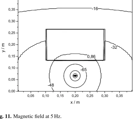
In a next step, one conducting bar of quadratic cross-section with a=b=0,1 m is placed at rq=(−0.1, −0.1) m. One single exciting line, carrying I=100 A, is placed at (0.0, −0.15) m, as shown in Fig. 8.

(5)

L. O. Fichte et al.: Shielding properties of a conducting bar calculated with a boundary integral method 123 PSfrag replacements

x/m

y/m

0.1 +0.3 0.1

0.3

0.05

s.

1.

5. CONCLUSIONS

representation for the vector potential in the exte-rior space from Green’s second theorem. Coupling these two equations for points on the contour of the bar resulted in a system of linear equations. The solution to this system delivered the coefficients de-scribing all fields. This method has been used to calculate the shielding properties of a conducting bar placed in the field of a exciting loop.

References

[1] Abramowitz, M.; Stegun, I.A.: Handbook of Mathematical Functions, New York 1970

[2] Hanson, G.W., Yakovlev, A.B.; Operator The-ory for Electromagnetics, Springer, New York 2002

[3] Ehrich, M.; Fichte, L.O.; L¨uer, M.: Contri-bution to Boundary Integrals by the Singu-larity of Kernels satisfying Helmholtz’ Equa-tion CJMW’2000 China-Japan Joint Meeting on Microwaves, Nanjing

[4] Fichte, L.O.; Ehrich, M.; Kurz, S.: An Ana-lytical Solution to the Eddy Current Problem of a Conducting Bar EMC 2004 International Symposium on Electromagnetic Compatibility, Sendai Conference Proceedings CD-ROM Fig. 12. Field attenuation at 5 Hz.

1Aa(and thereby the shielding effect of the conducting bar) is plotted in Fig. 10. The resulting plots are slightly non-symmetric because of roundoff-errors.

Figures 11 and 12 show the lines and the attenuation of the magnetic field for the same configuration and a significantly lower frequency ofω=51_s. Conductivity and permeability areκ=57·106 A_Vm, µri=1.

5 Conclusions

We applied a hybrid method to determine the field proper-ties of a rectangular conducting bar in the field of an exciting loop. While Helmholtz’ equation governing the vector po-tential inside the bar has been solved by separation, we ob-tained an integral representation for the vector potential in the exterior space from Green’s second theorem. Coupling these two equations for points on the contour of the bar re-sulted in a system of linear equations. The solution to this system delivered the coefficients describing all fields. This method has been used to calculate the shielding properties of a conducting bar placed in the field of a exciting loop.

References

Abramowitz, M. and Stegun, I. A.: Handbook of Mathematical Functions, New York 1970.

Ehrich, M., Fichte, L. O. and L¨uer, M.: Contribution to Bound-ary Integrals by the Singularity of Kernels satisfying Helmholtz’ Equation CJMW’2000 China-Japan Joint Meeting on Mi-crowaves, Nanjing, 2000.

Fichte, L. O., Ehrich, M., and Kurz, S.: An Analytical Solution to the Eddy Current Problem of a Conducting Bar EMC 2004 Inter-national Symposium on Electromagnetic Compatibility, Sendai Conference Proceedings CD-ROM, 2004.