R E S E A R C H
Open Access
Approximate solutions to variational
inequality over the fixed point set of a
strongly nonexpansive mapping
Shigeru Iemoto
1, Kazuhiro Hishinuma
2and Hideaki Iiduka
2**Correspondence: [email protected]
2Department of Computer Science, Meiji University, 1-1-1 Higashimita, Tama-ku, Kawasaki-shi, Kanagawa, 214-8571, Japan
Full list of author information is available at the end of the article
Abstract
Variational inequality problems over fixed point sets of nonexpansive mappings include many practical problems in engineering and applied mathematics, and a number of iterative methods have been presented to solve them. In this paper, we discuss a variational inequality problem for a monotone, hemicontinuous operator over the fixed point set of astronglynonexpansive mapping on a real Hilbert space. We then present an iterative algorithm, which uses the strongly nonexpansive mapping at each iteration, for solving the problem. We show that the algorithm potentially converges in the fixed point set faster than algorithms using firmly nonexpansive mappings. We also prove that, under certain assumptions, the
algorithm with slowly diminishing step-size sequences converges to a solution to the problem in the sense of the weak topology of a Hilbert space. Numerical results demonstrate that the algorithm converges to a solution to a concrete variational inequality problem faster than the previous algorithm.
MSC: 47H06; 47J20; 47J25
Keywords: variational inequality problem; fixed point set; strongly nonexpansive mapping; monotone operator
1 Introduction
The paper presents an iterative algorithm for the variational inequality problem [–] for a monotone, hemicontinuous operatorAover a nonempty, closed convex subsetCof a real Hilbert spaceHwith inner product·,·and its induced norm · ,
findz∈Csuch thaty–z,Az ≥ for ally∈C. ()
Problem () can be solved by using convex optimization techniques. A typical iterative procedure for Problem () is theprojected gradient method[, ], and it is expressed as
x∈Candxn+=PC(I–rnA)xnforn= , , . . . , wherePCstands for the metric projection ontoC,Iis the identity mapping onH, and{rn} ⊂(,∞). However, as the method requires repetitive use ofPC, it can only be applied when the explicit form ofPCis known (e.g.,Cis a closed ball or a closed cone). The following method, called thehybrid steepest descent method(HSDM) [], enables us to consider the case in whichChas a more complicated
form:x∈Hand
xn+= (I–rnA)Txn
for alln= , , . . . , where {rn} ⊂(, ] andT: H→H is an easily implemented nonex-pansive mapping satisfyingFix(T) :={x∈H:Tx=x}=C. HSDM converges strongly to a unique solution to the variational inequality problem overFix(T),
findz∈Fix(T) such thaty–z,Az ≥ for ally∈Fix(T), ()
whenA:H→His strongly monotone and Lipschitz continuous. Problem () contains many applications such as signal recovery problems [], beam-forming problems [], power-control problems [, ], bandwidth allocation problems [–], and optimal control problems []. References [, ], and [] presented acceleration methods for solving Problem () whenAis strongly monotone and Lipschitz continuous. Algorithms were presented to solve Problem () whenAis (strictly) monotone and Lipschitz continu-ous [, ]. WhenH=RN andA: RN→RN is continuous (and is not necessarily mono-tone), a simple algorithm,xn+:=αnxn+ ( –αn)(/)(I+T)(xn–rnAxn) (αn,rn∈[, ]), was presented in [] and the algorithm converges to a solution to Problem () under some conditions.
Reference [] proposed an iterative algorithm for solving Problem () whenA:H→H
is monotone and hemicontinuous and showed that the algorithm weakly converges to a solution to the problem under certain assumptions. The results in [] are summarized as follows: suppose thatF:H→His a firmly nonexpansive mapping withFix(F)=∅and thatA:H→His a monotone, hemicontinuous mapping with
VIFix(F),A:=z∈Fix(F) :y–z,Az ≥ for ally∈Fix(F)=∅.
Define a sequence{xn} ⊂Hbyx∈Hand
⎧ ⎨ ⎩
yn=F(I–rnA)xn,
xn+=αnxn+ ( –αn)yn
()
for all n = , , . . . , where {αn} ⊂ [, ) and {rn} ⊂(, ). Assume that {Axn} in algo-rithm () is bounded, and that there existsn∈Nsuch thatVI(Fix(F),A)⊂:= ∞n=n{x∈
Fix(F) :xn–x,Axn ≥}. If{αn} and{rn} satisfylim supn→∞αn< ,
∞
n=rn<∞, and
limn→∞xn–yn/rn= , then{xn}weakly converges to a point inVI(Fix(F),A). To relax the strong monotonicity condition ofAconsidered in [], afirmly nonexpansive mapping Fis used in algorithm () in place of a nonexpansive mappingT. From the fact that a firmly nonexpansive mappingFcan be represented by the form,F= (/)(I+T), for some non-expansive mappingT, algorithm () whenαn:= andF:= (/)(I+T) can be simplified as follows:x∈Hand
xn+=
(I+T)(xn–rnAxn) =
(xn–rnAxn) +
In constrained optimization problems, one is required to satisfy constraint conditions early in the process of executing an iterative algorithm. From this viewpoint, we intro-duce the following algorithm with a weighted parameterα, which is more than /:
xn+= ( –α)(xn–rnAxn) +αT(xn–rnAxn)
=( –α)I+αT(xn–rnAxn) =:S(xn–rnAxn). ()
Algorithm () potentially converges in the fixed point set faster than algorithm (). Here, we can see that the mapping,S:= ( –α)I+αT, satisfies thestrong nonexpansivity con-dition [], which is a weaker concon-dition than firm nonexpansivity. This implies that the previous algorithms in [, ], which can be applied to Problem () when T is firmly nonexpansive, cannot solve Problem () whenT is strongly nonexpansive.
In this paper, we present an iterative algorithm for solving the variational inequality problem with a monotone, hemicontinuous operator over the fixed point set of a strongly nonexpansive mapping and show that the algorithm weakly converges to a solution to the problem under certain assumptions.
The rest of the paper is organized as follows. Section covers the mathematical prelim-inaries. Section presents the algorithm for solving the variational inequality problem for a monotone, hemicontinuous operator over the fixed point set of a strongly nonexpansive mapping, and its convergence analyses. Section provides numerical comparisons of the algorithm with the previous algorithm in [] and shows that the algorithm converges to a solution to a concrete variational inequality problem faster than the previous algorithm. Section concludes the paper.
2 Preliminaries
Throughout this paper, we will denote the set of all positive integers byNand the set of all real numbers byR. LetHbe a real Hilbert space with inner product·,·and its induced norm · . We denote the strong convergence and weak convergence of{xn}tox∈Hby
xn→xandxnx, respectively. It is well known thatHsatisfies the following condition, calledOpial’s condition[]: for any{xn} ⊂Hsatisfyingxnx,lim infn→∞xn–x< lim infn→∞xn–yholds for ally∈H withy=x; see also [, , ]. To prove our main
theorems, we need the following lemma, which was proven in []; see also [, , ].
Lemma .([]) Assume that{sn}and{en}are sequences of non-negative numbers such
that sn+≤sn+enfor all n∈N.If
∞
n=en<∞,thenlimn→∞snexists.
2.1 Strong nonexpansivity and fixed point set
LetT be a mapping ofH into itself. We denote the fixed point set ofT byFix(T);i.e.,
Fix(T) ={z∈H:Tz=z}. A mappingT:H→His said to benonexpansiveifTx–Ty ≤
x–yfor allx,y∈H.Fix(T) is closed and convex whenT is nonexpansive [, , , ].
T:H→His said to bestrongly nonexpansive[] ifTis nonexpansive and if, for bounded sequences{xn},{yn} ⊂H,xn–yn–Txn–Tyn → impliesxn–yn– (Txn–Tyn) →. The following properties for strongly nonexpansive mappings were shown in []:
• A strongly nonexpansive mapping,T:H→H, withFix(T)=∅isasymptotically regular[, ],i.e., for eachx∈H,limn→∞Tnx–Tn+x= .
• IfS,T:H→Hare strongly nonexpansive, thenST is also strongly nonexpansive, and
Fix(ST) =Fix(S)∩Fix(T)whenFix(S)∩Fix(T)=∅.
• IfS:H→His strongly nonexpansive and ifT:H→His nonexpansive, then
αS+ ( –α)Tis strongly nonexpansive forα∈(, ). IfFix(S)∩Fix(T)=∅, then
Fix(αS+ ( –α)T) =Fix(S)∩Fix(T)[]. In particular, since the identity mappingIis strongly nonexpansive, the mappingU:=αI+ ( –α)Tis strongly nonexpansive. Such
Uis said to beaveraged nonexpansive.
Example . LetD⊂Hbe a closed convex set, which is simple in the sense thatPDcan be calculated explicitly. Furthermore, letf:H→Rbe Fréchet differentiable and∇f:H→H
be Lipschitz continuous;i.e., there existsL> such that∇f(x) –∇f(y) ≤Lx–yfor allx,y∈H. Then, forr∈(, /L],Sr:=PD(I–r∇f) is nonexpansive [], [, Lemma .]. DefineT:H→Hby
T:=αI+ ( –α)Sr
α∈(, ). ()
ThenT is strongly nonexpansive andFix(T) ={x∈D:f(x) =miny∈Df(y)}.
Example . LetDi⊂H (i= , , . . . ,m) be a closed convex set, which is simple in the sense thatPDican be calculated explicitly. Define(x) := (/)
m
i=ωid(x,Di) for allx∈H, whereωi∈(, ) with
m
i=ωi= andd(x,Di) :=min{x–y: y∈Di}(i= , , . . . ,m). Also, we defineS:H→HandT:H→Has
S:=PD
m
i= ωiPDi
, T:=αI+ ( –α)S α∈(, ). ()
ThenSis nonexpansive [, Proposition .] andFix(S) =C:={x∈D:(x) =miny∈D(y)}. Hence,Tis strongly nonexpansive andFix(T) =C.Cis referred to as ageneralized con-vex feasible set[, ] and is defined as the subset ofDthat is closest toD,D, . . . ,Dmin the mean square sense. Even if mi=Di=∅,Cis well defined.C= mi=Diholds when
m
i=Di=∅. Accordingly,Cis a generalization of mi=Di.
A mappingF:H→His said to befirmly nonexpansive[] ifFx–Fy≤ x–y,Fx– Fyfor allx,y∈H(see also [, , ]). Every firmly nonexpansive mappingFcan be expressed asF= (/)(I+T) given some nonexpansive mappingT [, , ]. Hence, the class of averaged nonexpansive mappings includes the class of firmly nonexpansive mappings.
2.2 Variational inequality
An operatorA:H→His said to bemonotoneifx–y,Ax–Ay ≥ for allx,y∈H.A:H→ H is said to behemicontinuous[, p.] if, for anyx,y∈H, the mappingg: [, ]→H
defined by g(t) =A(tx+ ( –t)y) is continuous, whereH has a weak topology. LetCbe a nonempty, closed convex subset of H. Thevariational inequality problem[, ] for a monotone operatorA:H→His as follows (see also [, , –]):
We denote the solution set of the variational inequality problem byVI(C,A). The mono-tonicity and hemicontinuity ofAimply thatVI(C,A) ={z∈C:y–z,Ay ≥ for ally∈C}
[, Subsection .]. This means thatVI(C,A) is closed and convex.VI(C,A) is nonempty whenA:H→H is monotone and hemicontinuous, andC⊂His nonempty, compact, and convex [, Theorem ..].
Example . Letg: H→Rbe convex and continuously Fréchet differentiable andA:=
∇g. ThenAis monotone and hemicontinuous.
(i) Suppose thatf:H→Ris as in Example . andT:H→His defined as in () and setG:={z∈D: f(z) =minw∈Df(w)}. Then
VIFix(T),A=
x∈G:g(x) =min
y∈Gg(y)
.
A solution of this problem is a minimizer ofgover the set of all minimizers off overD. Therefore, the problem has a triplex structure [, , ].
(ii) Suppose thatT:H→His defined as in (). Then
VIFix(T),A=
x∈C:g(x) =min
y∈C
g(y)
.
This problem is to find a minimizer ofgover the generalized convex feasible set [, , , , ].
3 Optimization of variational inequality over fixed point set
In this section, we present an iterative algorithm for solving the variational inequality problem for a monotone, hemicontinuous operator over the fixed point set of a strongly nonexpansive mapping and its convergence analyses. We assume that T :H →H is a strongly nonexpansive mapping withFix(T)=∅and thatA:H→His a monotone, hemi-continuous operator.
Algorithm .
Step . Choosex∈H,r∈(, ), andα∈[, )arbitrarily, and letn:= .
Step . Givenxn∈H, choosern∈(, )andαn∈[, )and computexn+∈Has
yn:=T(xn–rnAxn), xn+:=αnxn+ ( –αn)yn.
Step . Updaten:=n+ , and go to Step .
To prove our main theorems, we need the following lemma.
Lemma . Suppose that{xn}is a sequence generated by Algorithm.and that{Axn}is
bounded.Moreover,assume that
(A) ∞n=rn<∞,or (B) ∞n=r
n<∞,VI(Fix(T),A)=∅,and the existence of ann∈Nsatisfying VI(Fix(T),A)⊂:= ∞n=n{x∈Fix(T) :xn–x,Axn ≥}.
Proof Putzn:=xn–rnAxnfor alln∈N. We first assume that condition (A) is satisfied and chooseu∈Fix(T) arbitrarily. Accordingly, we see that, for anyn∈N,
xn+–u=αnxn+ ( –αn)yn–u
≤αnxn–u+ ( –αn)zn–u
=αnxn–u+ ( –αn)(xn–u) –rnAxn
≤ xn–u+rnAxn. ()
From∞n=rn<∞, the boundedness of{Axn}, and Lemma ., the limit of{xn–u}exists for allu∈Fix(T), which implies that{xn}is bounded.
Next, suppose that condition (B) is satisfied, and letu∈Fix(T). Then, from the mono-tonicity ofA, we find that, for anyn∈N,
xn+–u=αnxn+ ( –αn)yn–u
≤αnxn–u+ ( –αn)yn–u
≤αnxn–u+ ( –αn)zn–u
=αnxn–u+ ( –αn)(xn–u) –rnAxn
=αnxn–u+ ( –αn)
xn–u+ rnu–xn,Axn+rnAxn
≤ xn–u+ ( –αn)
rnu–xn,Axn+Krn
=xn–u+ ( –αn)
rnu–xn,Axn–Au
+ rnu–xn,Au+Krn
≤ xn–u+ rn( –αn)u–xn,Au+Krn, ()
whereK:=sup{Axn:n∈N}<∞. Especially in the case ofu∈VI(Fix(T),A)⊂, it follows from condition (B) that, for anyn≥n,
xn+–u≤ xn–u+ rn( –αn)u–xn,Axn+Krn
≤ xn–u+Krn.
Hence, the condition,∞n=rn<∞, and Lemma . guarantee that the limit of{xn–u} exists for allu∈VI(Fix(T),A). We thus conclude that{xn}is bounded.
Now, we are in the position to perform the convergence analysis on Algorithm . under condition (A) in Lemma ..
Theorem . Let{xn}be a sequence generated by Algorithm.and assume that{Axn}is
bounded and that the sequences{αn} ⊂[, )and{rn} ⊂(, )satisfy
lim sup
n→∞ αn< , ∞
n=
rn<∞, and n→∞lim xn –yn
rn = .
Proof Putzn:=xn–rnAxnfor alln∈N. The proof consists of the following steps: (a) Prove that{xn}and{zn}are bounded.
(b) Prove thatlimn→∞xn–yn= andlimn→∞xn–Txn= hold. (c) Prove that{xn}converges weakly to a point inVI(Fix(T),A).
(a) Chooseu∈Fix(T) arbitrarily. From the inequality,zn–u=(xn–rnAxn) –u ≤
xn–u+rnAxn, and Lemma ., we deduce that{zn}is bounded.
(b) Putc:=limn→∞xn–ufor anyu∈Fix(T). Then, from∞n=rn<∞, for anyε> , we can choosem∈Nsuch that|xn–u–c| ≤ε, andrn≤εfor alln≥m. Also, there existsa> such thatαn<a< for alln≥mbecause of lim supn→∞αn< . Sinceyn= (/( –αn))xn+– (αn/( –αn))xn, we have
yn–u ≥ –αnxn+
–u– αn –αnxn
–u
for alln∈N. We find that, for anyn≥m,
yn–u ≥ –αn
(c–ε) – αn –αn
(c+ε) =c– +αn –αn
ε≥c– +a –aε.
Hence, for anyu∈Fix(T) and for anyn≥m, we have
≤ zn–u–Tzn–Tu ≤ xn–u+rnAxn–yn–u
≤c+ε+√Kε–
c– +a –aε
=
–a+
√ K
ε,
whereK=sup{Axn:n∈N}<∞, which implies thatlimn→∞(zn–u–Tzn–Tu) = . SinceTis strongly nonexpansive, we get
lim
n→∞(zn–u) – (Tzn–u)=n→∞limzn–Tzn=n→∞lim zn–yn= . ()
From () andxn–zn=rnAxn → asn→ ∞, we also get
lim
n→∞xn–yn= . ()
Fromxn–Txn ≤ xn–yn+yn–Txn ≤ xn–yn+zn–xn, and (), we deduce that
lim
n→∞xn–Txn= . ()
(c) From the boundedness of{xn}, there exists a subsequence{xni}of{xn}such that{xni} converges weakly to a pointv∈H. From the nonexpansivity ofTand (), it is guaranteed thatT is demiclosed (i.e.,xnuandxn–Txn → implyu∈Fix(T)). Hence, we have
v∈Fix(T). From (), we get, for anyu∈Fix(T) and for anyn∈N,
≤xn–u+xn+–u
xn–u–xn+–u
which means
≤Lxn–xn+
rn
+ ( –αn)u–xn,Au+Krn
=L( –αn)xn–yn
rn
+ ( –αn)u–xn,Au+Krn
≤Lxn–yn
rn
+ ( –αn)u–xn,Au+Krn,
where L:=sup{xn–u+xn+ –u: n∈N}<∞. From xn–yn/rn→, xnv,
lim supnαn< , andrn→, we have
≤ u–v,Au for allu∈Fix(T).
The monotonicity and hemicontinuity ofAimply thatv∈VI(Fix(T),A). Finally, we show that{xn}converges weakly tov∈VI(Fix(T),A). Assume that another subsequence{xnj}of {xn}converges weakly tow. Then, from the discussion above, we also getw∈VI(Fix(T),A). Ifv=w, Opial’s theorem [] guarantees that
lim
n→∞xn–v=i→∞limxni–v
<lim
i→∞xni–w
= lim
n→∞xn–w
=lim
j→∞xnj–w
<lim
j→∞xnj–v
= lim
n→∞xn–v.
This is a contradiction. Thus, v=w. This implies that every subsequence of {xn} con-verges weakly to the same point in VI(Fix(T),A). Therefore, {xn} converges weakly to
v∈VI(Fix(T),A). This completes the proof.
Remark . The numerical examples in [, , ] show that Algorithm . satisfies
limn→∞xn–yn/rn= whenT is firmly nonexpansive andrn:= /nα(≤α< ).
How-ever, whenα≥, there are counterexamples that do not satisfylimn→∞xn–yn/rn= [, , ].
Remark . If the sequence{xn}satisfies the assumptions in Theorem ., we need not assume thatVI(Fix(T),A)=∅or thatn∈Nexists such thatVI(Fix(T),A)⊂in
condi-tion (B) (see also [, Remark (c)]).
Remark . Let us provide the sufficient condition of the boundedness of{Axn}. Suppose thatFix(T) is bounded andAis Lipschitz continuous. Then we can set a bounded setV
can compute
xn+:=PV
αnxn+ ( –αn)yn
(n= , , . . .) ()
instead ofxn+in Algorithm .. Since{xn} ⊂V andV is bounded,{xn}is bounded. The Lipschitz continuity ofAmeans thatAxn–Ax ≤Lxn–x(x∈H), whereL(> ) is a constant, and hence,{Axn}is bounded. We can prove that Algorithm . with Equation () and{αn}and{rn}satisfying the conditions in Theorem . (or Theorem .) weakly converges to a point inVI(Fix(T),A) by referring to the proof of Theorem . (or Theo-rem .).
We prove the following theorem under condition (B) in Lemma .. The essential parts of a proof are similar those of Lemma . and Theorem ., so we will only give an outline of the proof below.
Theorem . Let{xn}be a sequence generated by Algorithm ..Assume that{Axn}is
bounded and that{αn} ⊂[, )and{rn} ⊂(, )satisfy
lim sup
n→∞ αn< , ∞
n=
rn<∞, and lim
n→∞
xn–yn
rn = .
IfVI(Fix(T),A)=∅and if there exists n∈Nsuch thatVI(Fix(T),A)⊂ n∞=n{x∈Fix(T) :
xn–x,Axn ≥},then the sequence{xn}converges weakly to a point inVI(Fix(T),A).
Proof Putzn:=xn–rnAxnfor alln∈N. As in the proof of Theorem ., we proceed with the following steps:
(a) Prove that{xn}and{zn}are bounded. (b) Prove thatlimn→∞xn–Txn= holds.
(c) Prove that{xn}converges weakly to a point inVI(Fix(T),A).
(a) From Lemma ., it follows that the limit of{xn–u}exists for allu∈VI(Fix(T),A), and hence{xn}and{zn}are bounded.
(b) Letu∈VI(Fix(T),A) and putc:=limn→∞xn–u. Since
∞
n=rn<∞, the condition,
rn→, holds. As in the proof of Theorem .(b), for anyε> , there existsm∈Nsuch that
xn–u–c≤ε, and yn–u ≥c– +a
–aε
for alln≥m. Bylim supn→∞αn< , there existsa> such thatαn<a< . Since the in-equalityzn–u=(xn–rnAxn) –u ≤ xn–u+rnAxnholds, we have
≤ zn–u–Tzn–Tu
≤ xn–u+rnAxn–yn–u
≤c+ε+√Kε–
c– +a –aε
=
–a+
√ K
whereK=sup{Axn:n∈N}<∞. This implies thatlimn→∞(zn–u–Tzn–Tu) = . From the strong nonexpansivity ofT, we getlimn→∞zn–Tzn= . The rest of the proof is the same as the proof of Theorem .(b). Accordingly, we obtainlimn→∞xn–Txn= . (c) Following the proof of Theorem .(c), there exists a subsequence{xni} ⊂ {xn}such that{xni}converges weakly tov∈VI(Fix(T),A). Assume that another subsequence{xnj}of {xn}converges weakly tow. Then we also havew∈VI(Fix(T),A). Since the limit of{xn–
u}exists foru∈VI(Fix(T),A), Opial’s theorem [] guarantees thatv=w. This implies that every subsequence of{xn}converges weakly to the same point inVI(Fix(T),A), and hence,{xn}converges weakly tov∈VI(Fix(T),A). This completes the proof.
As we mentioned in Section , to solve constrained optimization problems whose fea-sible set is the fixed point set of a nonexpansive mappingT, Algorithm . must converge inFix(T) early in the execution. Therefore, it would be useful to use a large parameterα
(∈(, )) when a strongly nonexpansive mapping is represented by ( –α)I+αT. Theo-rem . has the following consequences.
Corollary . Let T:H→H be a nonexpansive mapping withFix(T)=∅and let A:H→ H be a monotone,hemicontinuous mapping.Let{xn}be a sequence generated by x∈H and
⎧ ⎨ ⎩
yn= (( –α)I+αT)(xn–rnAxn),
xn+=αnxn+ ( –αn)yn
()
for all n∈N,where{αn} ⊂[, ),α∈(, )and{rn} ⊂(, ).Assume that{Axn}is a bounded
sequence and that
lim sup
n→∞ αn< , ∞
n=
rn<∞, and n→∞lim xn –yn
rn = .
Then{xn}converges weakly to a point inVI(Fix(T),A).
Proof Since every averaged nonexpansive mapping is strongly nonexpansive andFix(( –
α)I+αT) =Fix(T) forα∈(, ), Theorem . implies Corollary ..
By following the proof of Theorem . and Corollary ., we get the following.
Corollary . Let T :H→H be a nonexpansive mapping with Fix(T)=∅ and let A:
H→H be a monotone,hemicontinuous mapping.Let{xn}be a sequence in algorithm().
Assume that{Axn}is a bounded sequence and that
lim sup
n→∞ αn< , ∞
n=
rn<∞, and lim
n→∞
xn–yn
rn = .
IfVI(Fix(T),A)=∅and if there exists n∈Nsuch thatVI(Fix(T),A)⊂ ∞n=n{x∈Fix(T) :
4 Numerical examples
Let us apply Algorithm . and the algorithm in [] to the following variational inequality problem.
Problem . Definef:R,→RandC
i(⊂R,) (i= , ) by
f(x) := x,Qx
x∈R,,
Ci:=
x∈R,:ai,x ≤bi
(i= , ),
whereQ∈R,×,is positive semidefinite,a
i:= (a()i ,a
()
i , . . . ,a
(,)
i )∈R,, andbi∈
R+(i= , ). Findz∈VI(C∩C,∇f).
We set Q as a diagonal matrix with diagonal components , , . . . , and choose
a(ij)∈(, ) (i= , ,j= , , . . . , ,) to be Mersenne Twister pseudo-random num-bers given by therandom-realfunction of srfi-, Gauche.a We also setb
:= ,
andb:= ,. The compiler used in this experiment was gcc.bThe double-precision
floating points were used for arithmetic processing of real numbers. The language was C. In the experiment, we used the following algorithm:
⎧ ⎨ ⎩
yn:= (( –α)I+αPCPC)(xn– –
(n+).∇f(xn)),
xn+:=xn+yn (n∈N),
()
where α∈(, ). Note that the projectionPCi (i= , ) can be computed within a finite
number of arithmetic operations [, p.] becauseCi(i= , ) is halfspace. More pre-cisely,
PCi(x) =x+
min{,bi–ai,x}
ai
ai
x∈R,,i= , .
We can see that algorithm () with α:= / coincides with the previous algorithm in []. Hence, we comparecalgorithm () withα:= / with algorithm () withα:= / and verify that algorithm () with α:= / converges inC∩C =Fix(PCPC) faster than algorithm () withα:= /. We selected one hundred initial pointsx=x(k)∈R,
(k= , , . . . , ) as pseudo-random numbers generated by therandfunction of the C Standard Library. We executed algorithm () withα:= / and algorithm () withα:= / for these initial points. Let{xn(k)}be the sequence generated byx(k) and algorithm (). Here, we define
Dn:=
k=
xn(k) –PCPC
xn(k) (n∈N).
The convergence of{Dn}to implies that algorithm () converges to a point inC∩C.
Corollary . guarantees that algorithm () converges to a solution to Problem . if
{∇f(xn)}is bounded and if
lim
n→∞(n+ )
.x
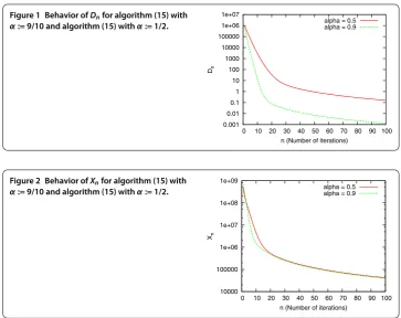
Figure 1 Behavior ofDnfor algorithm (15) with
α:= 9/10 and algorithm (15) withα:= 1/2.
Figure 2 Behavior ofXnfor algorithm (15) with
α:= 9/10 and algorithm (15) withα:= 1/2.
To verify whether algorithm () satisfies condition (), we employed
Xn:=
k=
(n+ ).xn(k) –yn(k) (n∈N),
where yn(k) := (( –α)I+αPCPC)(xn(k) – (–/(n+ ).)∇f(xn(k))) (k= , , . . . , ,
n∈N). The convergence of{Xn}to implies that algorithm () satisfies condition (). We also used
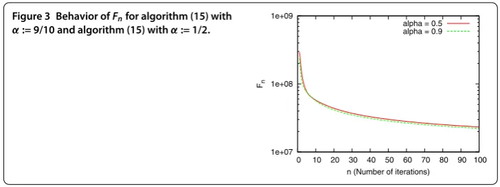
Fn:=
k= fxn(k)
(n∈N)
to check that algorithm () is stable.
Figure indicates the behaviors ofDnfor algorithm () withα:= / and algorithm () withα:= /. This figure shows that{Dn}in algorithm () withα:= / converges to faster than{Dn}in algorithm () withα:= /;i.e., algorithm () withα:= / converges inC∩Cfaster than the previous algorithm in [].
Figure compares the behaviors ofXnfor algorithm () withα:= / and algorithm () withα:= / and shows that the{Xn}generated by each algorithm converges to ;i.e., they each satisfy (). Therefore, from Corollary ., we can conclude that they can find a solution to Problem ..
Figure 3 Behavior ofFnfor algorithm (15) with
α:= 9/10 and algorithm (15) withα:= 1/2.
potentially converges in the constraint setC∩Cfaster than the previous algorithm in
[] withα:= /.
5 Conclusion
We studied a variational inequality problem for a monotone, hemicontinuous operator over the fixed point set of a strongly nonexpansive mapping in a Hilbert space and de-vised an iterative algorithm for solving it. Our convergence analyses guarantee that the algorithm weakly converges to a solution under certain assumptions. We gave numerical results to support the convergence analyses on the algorithm. The results showed that the algorithm converges to a solution to a concrete variational inequality problem faster than the previous algorithm.
Competing interests
The authors declare that they have no competing interests.
Authors’ contributions
All authors contributed equally to the writing of this paper. All authors read and approved the final manuscript.
Author details
1Chuo University Suginami High School, 2-7-1 Imagawa, Suginami-ku, Tokyo, 167-0035, Japan.2Department of Computer Science, Meiji University, 1-1-1 Higashimita, Tama-ku, Kawasaki-shi, Kanagawa, 214-8571, Japan.
Acknowledgements
We are sincerely grateful to the Lead Guest Editor, Qamrul Hasan Ansari, of Special Issue on Variational Analysis and Fixed Point Theory: Dedicated to Professor Wataru Takahashi on the occasion of his 70th birthday, and the two anonymous referees for helping us improve the original manuscript. This work was supported by the Japan Society for the Promotion of Science through a Grant-in-Aid for JSPS Fellows (08J08592) and a Grant-in-Aid for Young Scientists (B) (23760077).
Endnotes
a We used the Gauche scheme shell, 0.9.3.3 [utf-8,pthreads], x86_64-apple-darwin12.4.1. b We used gcc version 4.2.1 (Based on Apple Inc. build 5658) (LLVM build 2336.11.00). c For example, we set a large parameter,i.e., much more than 1/2:α= 9/10.
Received: 3 September 2013 Accepted: 13 February 2014 Published:25 Feb 2014
References
1. Kinderlehrer, D, Stampacchia, G: An Introduction to Variational Inequalities and Their Applications. Academic Press, New York (1980)
2. Lions, J-L, Stampacchia, G: Variational inequalities. Commun. Pure Appl. Math.20, 493-519 (1967) 3. Rockafellar, RT, Wets, RJ-B: Variational Analysis. Springer, Berlin (1998)
4. Stampacchia, G: Formes bilinéaires coercitives sur les ensembles convexes. C. R. Math. Acad. Sci. Paris258, 4413-4416 (1964)
5. Takahashi, W: Nonlinear Functional Analysis. Fixed Point Theory and Its Applications. Yokohama Publishers, Yokohama (2000)
9. Goldstein, AA: Convex programming in Hilbert space. Bull. Am. Math. Soc.70, 709-710 (1964)
10. Yamada, I: The hybrid steepest descent method for the variational inequality problem over the intersection of fixed point sets of nonexpansive mappings. In: Inherently Parallel Algorithms in Feasibility and Optimization and Their Applications (Haifa, 2000). Stud. Comput. Math., vol. 8, pp. 473-504. North-Holland, Amsterdam (2001)
11. Combettes, PL: A block-iterative surrogate constraint splitting method for quadratic signal recovery. IEEE Trans. Signal Process.51, 1771-1782 (2003)
12. Slavakis, K, Yamada, I: Robust wideband beamforming by the hybrid steepest descent method. IEEE Trans. Signal Process.55, 4511-4522 (2007)
13. Iiduka, H, Yamada, I: An ergodic algorithm for the power-control games for CDMA data networks. J. Math. Model. Algorithms8, 1-18 (2009)
14. Iiduka, H: Fixed point optimization algorithm and its application to power control in CDMA data networks. Math. Program.133, 227-242 (2012)
15. Iiduka, H: Fixed point optimization algorithm and its application to network bandwidth allocation. J. Comput. Appl. Math.236, 1733-1742 (2012)
16. Iiduka, H: Iterative algorithm for triple-hierarchical constrained nonconvex optimization problem and its application to network bandwidth allocation. SIAM J. Optim.22, 862-878 (2012)
17. Iiduka, H: Fixed point optimization algorithms for distributed optimization in networked systems. SIAM J. Optim.23, 1-26 (2013)
18. Iiduka, H, Yamada, I: Computational method for solving a stochastic linear-quadratic control problem given an unsolvable stochastic algebraic Riccati equation. SIAM J. Control Optim.50, 2173-2192 (2012)
19. Iiduka, H: Acceleration method for convex optimization over the fixed point set of a nonexpansive mapping. Math. Program. (2014). doi:10.1007/s10107-013-0741-1
20. Iiduka, H, Yamada, I: A use of conjugate gradient direction for the convex optimization problem over the fixed point set of a nonexpansive mapping. SIAM J. Optim.19, 1881-1893 (2009)
21. Iiduka, H: A new iterative algorithm for the variational inequality problem over the fixed point set of a firmly nonexpansive mapping. Optimization59, 873-885 (2010)
22. Bruck, RE, Reich, S: Nonexpansive projections and resolvents of accretive operators in Banach spaces. Houst. J. Math. 3, 459-470 (1977)
23. Opial, Z: Weak convergence of the sequence of successive approximations for nonexpansive mappings. Bull. Am. Math. Soc.73, 591-597 (1967)
24. Goebel, K, Kirk, WA: Topics in Metric Fixed Point Theory. Cambridge University Press, Cambridge (1990) 25. Tan, KK, Xu, HK: Approximating fixed points of nonexpansive mappings by the Ishikawa iteration process. J. Math.
Anal. Appl.178, 301-308 (1993)
26. Berinde, V: Iterative Approximation of Fixed Points. Lecture Notes in Mathematics. Springer, Berlin (2007)
27. Goebel, K, Reich, S: Uniform Convexity, Hyperbolic Geometry, and Nonexpansive Mappings. Dekker, New York (1984) 28. Browder, FE, Petryshyn, WV: The solution by iteration of linear functional equations in Banach spaces. Bull. Am. Math.
Soc.72, 566-570 (1966)
29. Aoyama, K, Kimura, Y, Takahashi, W, Toyoda, M: On a strongly nonexpansive sequence in Hilbert spaces. J. Nonlinear Convex Anal.8, 471-489 (2007)
30. Baillon, J-B, Haddad, G: Quelques propriétés des opérateurs angle-bornés etn-cycliquement monotones. Isr. J. Math. 26, 137-150 (1977)
31. Iiduka, H: Strong convergence for an iterative method for the triple-hierarchical constrained optimization problem. Nonlinear Anal.71, 1292-1297 (2009)
32. Combettes, PL, Bondon, P: Hard-constrained inconsistent signal feasibility problems. IEEE Trans. Signal Process.47, 2460-2468 (1999)
33. Browder, FE: Convergence theorems for sequences of nonlinear operators in Banach spaces. Math. Z.100, 201-225 (1967)
34. Reich, S, Shoikhet, D: Nonlinear Semigroups, Fixed Points, and Geometry of Domains in Banach Spaces. Imperial College Press, London (2005)
35. Iiduka, H: Iterative algorithm for solving triple-hierarchical constrained optimization problem. J. Optim. Theory Appl. 148, 580-592 (2011)
36. Bauschke, HH, Borwein, JM: On projection algorithms for solving convex feasibility problems. SIAM Rev.38, 367-426 (1996)
10.1186/1687-1812-2014-51