The Thirty-Third AAAI Conference on Artificial Intelligence (AAAI-19)
Learning Heterogeneous Spatial-Temporal Representation
for Bike-Sharing Demand Prediction
Youru Li,
†,‡Zhenfeng Zhu,
†,‡Deqiang Kong,
≡Meixiang Xu,
†,‡Yao Zhao
†,‡†Institute of Information Science, Beijing Jiaotong University, Beijing, China
‡Beijing Key Laboratory of Advanced Information Science and Network Technology, Beijing, China ≡Microsoft Multimedia, Beijing, China
†,‡{liyouru,zhfzhu,xumx0721,yzhao}@bjtu.edu.cn,≡[email protected]
Abstract
Bike-sharing systems, aiming at meeting the public’s need for ”last mile” transportation, are becoming popular in re-cent years. With an accurate demand prediction model, shared bikes, though with a limited amount, can be effectively uti-lized whenever and wherever there are travel demands. De-spite that some deep learning methods, especially long short-term memory neural networks (LSTMs), can improve the performance of traditional demand prediction methods only based on temporal representation, such improvement is lim-ited due to a lack of mining complex spatial-temporal re-lations. To address this issue, we proposed a novel model named STG2Vec to learn the representation from heteroge-neous spatial-temporal graph. Specifically, we developed an event-flow serializing method to encode the evolution of dy-namic heterogeneous graph into a special language pattern such as word sequence in a corpus. Furthermore, a dynamic attention-based graph embedding model is introduced to ob-tain an importance-awareness vectorized representation of the event flow. Additionally, together with other multi-source information such as geographical position, historical transi-tion patterns and weather,e.g., the representation learned by STG2Vec can be fed into the LSTMs for temporal modeling. Experimental results from Citi-Bike electronic usage records dataset in New York City have illustrated that the proposed model can achieve competitive prediction performance com-pared with its variants and other baseline models.
Introduction
Bike-Sharing systems have been widely used in urban pub-lic transportation due to their convenience and environmen-tal friendliness in recent years. As a representative product of the sharing economy, it is often hailed as a good helper to solve the ”last mile” in citizen transportation. Its users can check out a bike where they depart and return it to a sta-tion close to their destinasta-tion. However, due to the high fre-quency and randomness of using, the system has come to be unbalanced in bike distribution. This will result in short sup-ply of bikes in some places and oversupsup-ply in others, thus re-ducing user satisfaction. In general, to solve this unbalanced bike-sharing distribution problem, it is vital to propose an accurate demand prediction model.
Copyright c2019, Association for the Advancement of Artificial Intelligence (www.aaai.org). All rights reserved.
Bike-sharing demand prediction can usually be defined as a time series prediction problem from multi-source and heterogeneous data. Traditionally, time series prediction can be considered as building a suitable predictive model (Yule 1927) for a series of data points indexed in time order so as to make good use of the complex sequence dependencies. As a representative of the statistical regression methods, the auto-regressive moving average model (ARMA) and the auto-regressive integrated moving average (ARIMA) model (Box and Pierce 1968) are both well-known models for time series prediction. As machine learning methods grow pop-ular gradually, more researchers focused on the studies to establish nonlinear prediction model based on a large scale of historical data. Typical models such as the support vec-tor regression (SVR)(Drucker et al. 1996) based on kernel methods and the artificial neural networks (ANN) (Davoian and Lippe 2007) with strong nonlinear function approxima-tion ability and the k-Nearest Neighbor (K-NN) regression (Wang and Chaib-draa 2013) based on distance metric in feature space and some tree-based ensemble learning meth-ods, for instance, the random forests (RF) regression (Jo-hansson et al. 2014) and the gradient boosting regression tree (GBRT) (Li and Bai 2016).
With the rise of deep learning methods, the recurrent neu-ral network (RNN) (Rumelhart, Hinton, and Williams 1986) gradually becomes the state-of-the-art method for tempo-ral modeling. However, with longer driving sequence, some problems such as vanishing gradient limit the prediction ac-curacy of this model. To address these issue, the long short-term memory units (LSTM) (Hochreiter and Schmidhuber 1997) and its variants the gated recurrent unit (GRU) (Cho et al. 2014a) were proposed based on the original RNN which balances memorizing and forgetting by adding multi-ple threshold gates. Learning from cognitive neuroscience and inspired by some successful applications in natural language processing (Cho et al. 2014b), some researchers (Liang et al. 2018) introduce attention mechanisms to the encoding-decoding framework based on LSTMs to better se-lect from input series and encode information in long-term memory for time series prediction.
is greatly affected by external conditions. It is necessary to make full use of multi-source heterogeneous informa-tion in historical data. As a stainforma-tion-level predicinforma-tion prob-lem, it is vital to utilize the complex heterogeneous spatio-temporal graph which describes bicycle riding relationships. Inspired by some significant applications in unstructured data embedding (Mikolov et al. 2013) and structured data embedding (Zhu et al. 2013; Guo and Berkhahn 2016; Dai, Dai, and Song 2016) through deep learning meth-ods, we proposed a novel model named STG2Vec to learn the representation of heterogeneous spatio-temporal graph. Specifically, we proposed an event-flow serializing method to represent the evolution process of interaction between the current site and its neighbors from a heterogeneous graph structure within a time-step as a series. Furthermore, a dy-namic attention-based graph embedding model is proposed to obtain an importance-awareness vectorized representation of the event-flow.
In general, main contributions in this paper are:
• We developed an event-flow serializing method to repre-sent the evolution process of the dynamic heterogeneous graph as a series.
• A novel dynamic attention-based graph embedding model named STG2Vec is proposed to learn an importance-awareness vectorized representation from heterogeneous spatial-temporal graph.
• To better utilize the multi-source information, we intro-duced the CE-LSTM to combine the embedded multi-source information with the output of proposed STG2Vec for collaborative temporal modeling.
Related Work
With the wide application of bike-sharing in urban trans-portation, progress have been made in related researches ac-cordingly. Studies including data analysis and visualization (Yan et al. 2018), have employed data of bike-sharing tra-jectories to solve specific problems in urban management (Bao et al. 2017; He et al. 2018) and other areas. Demand prediction, as the most classic problem, has received the widest attention in this field. Based on predictive granu-larity, there are three groups of prediction models in ex-isting researches: city-level, cluster-level, and station-level. For the city-level and cluster-level groups, traditional meth-ods (Chen et al. 2016) usually predict the bike demand for a whole city or design a clustering algorithm to cluster bike stations into groups as prediction units. Although city-level or cluster-level does simplify the problem, it’s not as good as station-level prediction for bike-sharing managers to help when scheduling. However, the station-level prediction is difficult because the bike-sharing demand pattern of a sta-tion is highly dynamic and context-dependent.
Although station-level prediction is being challenged, it has attracted the attention of many researchers. In station-level hourly demand prediction tasks, some researchers fur-therly explore the external context data such as time factors and weather information together with feature engineering and model lightweight processing (Hulot, Aloise, and Jena
2018) for industrial applications. Others have made contri-bution to temporal modeling by introducing recurrent neural network (Chen et al. 2017) for bike-sharing demand predic-tion. Meanwhile, other researchers are interested in utiliz-ing the underlyutiliz-ing correlations between stations to predict the hourly demand at station-level with deep learning tech-niques such as graph convolutional neural network (GCN) together with the classic support vector regression model (Lin et al. 2017). Although above studies have improved the accuracy and efficiency of station-level demand prediction models in different ways, there is no way to align tempo-ral modeling with complex non-linear spatial-tempotempo-ral rela-tions mining.
In bike-sharing demand prediction, any stations are not isolated. The station establishes complex connections through riding relationships to each other which can be ex-pressed by graph structures. In order to capture complex non-linear spatial-temporal relations among stations, it is necessary to establish a length-fixed representation from graph structures. Embedding technology can usually obtain low-dimensional and length-fixed numeric vectors represen-tation from non-linear structures. Typically, the DeepWalk (Perozzi, Al-Rfou, and Skiena 2014) and node2vec (Grover and Leskovec 2016) are widely used in social network min-ing. These method were proposed inspired by some deep learning embedding methods which had led to significant progress in natural language processing (Mikolov et al. 2013). These make embedding methods used for represen-tation learning in data mining available.
In the specific problem, what is established by the rid-ing relationship among stations is a structurally unstable dy-namic heterogeneous graph structure. Although the above methods can learn the embedded representation of the graph structure, they are insufficient when extending to the dy-namic graph modeling. Naively applying existing embed-ding algorithms to each snapshot of dynamic graphs in-dependently usually leads to unsatisfactory performance in terms of stability, flexibility and efficiency. The study on dy-namic graphs embedding proposed a DynGEM model based on deep autoencoders (Goyal et al. 2018) which inspires a new idea for dynamic graph representation learning, but it still has room to improve when capturing dependencies be-tween each snapshots of dynamic graphs.
Preliminaries
In this section, we will introduce some notations and the definition of bike-sharing demand prediction. Bike-sharing demand prediction, as a time series prediction prob-lem, can be defined as a station-level check-out/in predic-tion issue. Given a set of historical trips records: TH = (Tr1, Tr2, . . . , TrH), where each tripTr = (Lo, Ld, τo, τd).
Specifically, whereLodenotes the start station, consists of
latitudeLo.latand longitudeLo.lon; whereLddenotes the
destination station, consists of latitudeLd.latand longitude
Ld.lon;τo andτdare the time corresponding to check-out
*OREDO
$WWQ*UDSK *OREDO
^d'ϮsĞĐ
^d'ϮsĞĐ ^d'ϮsĞĐ
D
D
D
/RFDO *UDSK
D
D
D
D
/RFDO $WWQ*UDSK
*UDSK
͘͘͘
͘͘͘
*OREDO
/RFDO $WWQ*UDSK
*UDSK
D
D
6 W WUDQV L
I IWUDQV6LW IWUDQV6LW7
IZHDW IWLPHW IZHDWIWLPHW IZHDW 7IWLPHW7
JUDSK6LW
I JUDSK6W
L
I IJUDSK6LW 7
W L
6 6LW 6LW7
L
; ;L ;7L
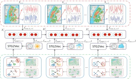
Figure 1: Graphical illustration of learning collaborative representation from nulti-source and heterogeneous spatial-temporal data. This figure is composed of three parts. The top part displays the process of learning historical transition patterns. The bottom part shows the Attn-Graph structure can be produced at the global level from the original graph which responds to the riding relationship between the central site and its neighbors at the current time interval extracted at the local level. Meanwhile, in the middle part of this figure, together with multi-source information from weather, time, geographical position and historical transition patterns, the representation learned by STG2Vec can be fed into the LSTMs for temporal modeling.
Table 1: Notations and Description In Task-level
Notation Description
Si Theithstation
OSi,t Check out of stationSiin timet
ISi,t Check in of stationSiin timet
ftrans,Si,t Feature of transition in ST-index
fwea,t Meteorology feature in timet
ftime,t Feature of time in timet
fgraph,Si,t Embedding of graph in ST-index
Given a set of historical trips which contains geographic and temporal information, we can predict theOSi,T+1and
ISi,T+1 of each station Si in next time interval by
ex-tracting feature of transition, meteorology, time and em-bedding of graph from each historical time intervals. Typ-ically, time series prediction usually uses a historical se-quence of values as the input data. Given jointly feature
Xi
t in time t and station Si which can be concatenated
by ftrans,Si,t,Fwea,t, ftime,t andfgraph,Si,t, the context
features at historical time intervals and stations can be de-fined as Xi = (X1i, X2i, ..., XTi), where X
i
t ∈ Xi and
Xti = (ftrans,Si,t, Fwea,t, ftime,t, fgraph,Si,t). Meanwhile,
historical values of check-out and check-in in each bike-sharing station yi = (y1i, yi2, ..., yTi) are also given. Gen-erally, we learn a nonlinear mapping function by using the historical context features Xi and its corresponding target valueyito obtain the predicted valuey˜i
T+1for check-out/in
respectively with the following formulation:
˜
yi
T+1=F(X
i, yi) (1)
where mappingF(·)is the nonliner mapping function we take for making prediction.
Methodology
6WDWLRQ,' /DW /RQ 7LPH 67,QGH[ * &RQFDWHQDWH &ODVVLILHU ^ƵďͲ'ƌĂƉŚŵďĞĚ 39'0 (YHQW)ORZ6HULDOL]H O W 39'0 39'0 * * N O W N O W + ')6 $WWHQWLRQ ͘͘͘ 3UH2UGHU 6LPLODULW\ 0HWULF 4XDQWL]DWLRQ (QFRGLQJ ͘͘͘ $WWQ*UDSK $WWHQWLRQ :HLJKW ')6 $WWHQWLRQ ͘͘͘ 3UH2UGHU 6LPLODULW\ 0HWULF 4XDQWL]DWLRQ (QFRGLQJ ͘͘͘ $WWQ*UDSK $WWHQWLRQ :HLJKW (PEHGGLQJ6SDFH ')6 3UH2UGHU (PEHGGLQJ6SDFH $WWHQWLRQ ͘͘͘ 6LPLODULW\ 0HWULF 4XDQWL]DWLRQ (QFRGLQJ ͘͘͘ $WWQ*UDSK $WWHQWLRQ :HLJKW (P
(PEHEHGGGGLQLQLQJJ6S6SDFDFHH
L N O 6 W
* L
N O 6 W * 7 L N O 6 W
* L
N O 6 W
*
7 L
O 6 W
* L
O 6 W * 7 L N O 6 W 9( L N O 6 W 9(P L N O 6 W ( 9 a L N O 6 W 9( L N O 6 W 9(P L N O 6 W ( 9a L O 6 W 9( L O 6 W 9(P L O 6 W ( 9a (PEHGGLQJ6SDFH
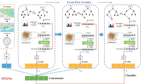
Figure 2: Graphical illustration of learning representation of attention-based heterogeneous spatial-temporal graph. The figure is composed of two parts. The top displays the process of event-flow serialize, and the bottom structure of STG2Vec. Event-flow serialize is the process of encoding the dynamic heterogeneous graph into a special language pattern such as sequence of words in a corpus. The STG2Vec takes dynamic attention-based graph embedding by event-flow series with the spatial-temporal index.
Mutil-Source Information Representation
Bike-sharing demand in station-level is affected by multiple complex factors, such as its geographical position and his-torical transition patterns, meteorology, time and correlation between its neighbors.
Firstly, we extracted the feature of transitionftrans,Si,tin
ST-index with statistical indicators such as total, mean, vari-ance, median, mode, minimum, and maximum in each time interval. Secondly, we defined time features for each time in stationSiasftime,t: rush or normal time of the day, day of
the week, week of the month, month of the season. Mean-while, as a kind of transportation, bike-sharing demand is affected by meteorology significantly. Thirdly, we define the meteorology feature in timetasfwea,t, which contains air
temperature, dew point temperature, relative humidity, wind speed, wind direction, visibility and weather condition type. In addition, the bike-sharing traffic of nearby stations can affect each other. Finally, to utilize this correlation between stations, we take embedding of the graph in ST-index by the STG2Vec we proposed.
Specifically, most attributes of meteorology and time fea-tures are categorical variables with sparse one-hot encod-ing. In order to achieve a dense representation of joint infor-mation, we transform the weather attributes with time-index into a low-dimensional vector by neural networks sim-ilar to sentence embedding (Le and Mikolov 2014).
Event-Flow Serialize
The event of bike-sharing checking may occur at any time, which makes the graph structure changing dynamically. The goal of language modeling is to estimate the likelihood of a specific sequence of words appearing in a corpus (Per-ozzi, Al-Rfou, and Skiena 2014). Event-flow serialize is the process to encode the evolution of dynamic heteroge-neous graph into a special language pattern such as word sequence in a corpus. Firstly, we divided a time interval (1h) by minutes. For instance, time intervalt = (t1, t2, ..., tl),
wherel∈[1, L]. Secondly, we traversed each unicom undi-rected sub-graph in Depth-First Search (DFS) and corre-sponding Depth-First Spanning Tree (DFST) can be ob-tained reseparately. For instance, in t and Si, the DFST:
T(GSi
tl)generated byG
i
tcan be traversed in Pre-order into
a node set V ESi
tl. It should be noted that each node can
be represented as a vector which consists of four parts: real-time net inflow, outflow, longitude and latitude. For instance, the node vector can be symbolized as nSi
tl =
(ISi,tl, OSi,tl, lon.Si, lat.Si).Meanwhile, we took
hierar-chical quantization encoding with inflow and outflow in each node to build a corpus with a reasonable frequency distribu-tion. Then, the event-flow series int andSi can be
repre-sented asV ESi
t = (V E Si
t1, ..., V E
Si
tl, ..., V E
Si
tL). The offline
corpus was established withV ESi
a new set of nodes can be find in the corpus by a hierarchi-cal search which consists of longth, location and quantitative level matching. Finally, the propose of event-flow serialize is to finish the information extraction of the evolution process of dynamic graph that is latent and spatially sensitive.
Dynamic Attention-based Graph Embedding
Graphical illustration of STG2Vec is given in Figure 2. In STG2Vec, outlined in Algoithm 1, the position information intis mapped to a unique vector as the spatial-temporal in-dex (ST-Inin-dex), represented by a column in matrixH and each set of nodes in corresponding graph within event-flow series can be seen as a special word is also mapped to a unique vector, represented by a column in matrix G. The ST-Index and the contextual special words are concatenated to predict the next word in fixed-length surroundings sam-pled from a sliding window over a event-flow series. Specif-ically, given a general spatial-temporal graph contextual se-riesV ESit1, ..., V E
Si
tl, ..., V E
Si
tL, the objective of STG2Vec
is to maximize the average log probability
1
L
L−k
X
t=k
logp(V ESi
tl|V E
Si
tl−k, ..., V E
Si
tl+k) (2)
The prediction task is typically done via a multiclass classi-fier, such as softmax. There, we have
p(V ESi
tl|V E
Si
tl−k, ..., V E
Si
tl+k) =
e
y
V Et−kSi
P
jeyj
(3)
Each ofyjis un-normalized log-probability for each output
intermediate graphj, computed as
y=b+U h(V ESi
tl−k, ..., V E
Si
tl+k;G) (4)
whereU, bare the softmax parameters.his constructed by a concatenation of intermediate graph vectors extracted from
Gand the ST-Index vector extracted fromH. In addition, we take stochastic gradient decent (SGD) to train the STG2Vec and the gradient obtained by backpropagation can be used to update parameters in our model.
Furthermore, to obtain an importance-awareness vector-ized representation of the event-flow, we use the attention mechanism to take importance-based sampling for the se-quence of nodes encoded by the event-flow serialize and train STG2Vec again with the new input of sampled nodes series. In addition, after training of STG2vec, the fixed-length vector representation formed by each node corre-sponding to different ST-Index can constitute an embedding space. Then we use the ST-Index as the key, and the cor-responding vector represents the value to construct a hash map. Specifically, for an instance, each node in the set of node V ESi
tl can obtained the corresponding fixed-length
vector representation by the hash map and these represen-tations can form a set of embedded representationV EmSi
tl.
Furthermore, we can get normalized attention weights by measuring the similarity of the length-fixed vector corre-sponding to each node one by one. Finally, the
attention-based graph V Eˆ Sti
l can be produced by importance-based
sampling fromV ESi
tl.
Algorithm 1STG2Vec (G,H,ω,d,τ,L) Require:
G: Event-flow series matrix, H: ST-Index matrix, ω: window size,d: embedding size,τ: training epochs,L: event-flow series length
Ensure:
fgraph,Si,t∈R
d: Embedding of graph in ST-index
1: whileiter= 1< τdo
2: Initialization: SampleΘandΦfromG,H
3: forV ESi
t ∈Θdo
4: V ESi
t ←(V E Si
t1, ..., V E
Si
tl , ..., V E
Si
tL)
5: forV ESi
tl ∈V E
Si
t do
6: αSi
tl ←CalAttnW eights(V E
Si
tl)
7: V ESi
tl ←
ˆ
V ESti
l ←α
Si
tl ·V E
Si
tl
8: end for
9: end for
10: PV-DM(Θ,Φ, ω, d) (Le and Mikolov 2014)
11: end while
Collaborative Temporal Modeling
To better utilize the external data and capture with com-plex non-linear spatial-temporal relations, we proposed the CE-LSTM. Together with multi-source information from weather, time, geographical position and historical transition patterns, the representation learned by STG2Vec can be fed into the LSTMs for collaborative temporal modeling.
Firstly, we define the jointly representation by concatenat-ing in each time interval and station as
Xti= (ftrans,Si,t, Fwea,t, ftime,t, fgraph,Si,t) (5)
Then,Xi = (Xi
1, X2i, ..., XTi)is fed into LSTM networks.
Furthermore, we can learn the nonliner mapping function by these formulation (Hochreiter and Schmidhuber 1997) of the calculating process in LSTM cells as follows:
it=σ(WxiXti+Whiht−1+Wcict−1+bi) (6)
ft=σ(WxfXti+Whfht−1+Wcfct−1+bf) (7)
ct=ftct−1+ittanh(WxcXti+Whcht−1+bc) (8)
ot=σ(WxoXti+Whoht−1+Wcoct−1+bo) (9)
ht=ottanh(ct) (10)
whereσ(·)represents the activation function of sigmoid and
W matrices with double subscript the connection weights between the two cells. In addition, itrepresents input gate state,ftforget gate state,ctcell state,otoutput gate andht
the hidden layer output in current time-step. Finally, we can take the last element of output vectorht−1as the predicted
value. It can be represented as:
˜
yi,t=ht−1 (11)
the final output value can be contacted to a vector:
˜
yi
T+1= (˜y
Experiments
In this section, we will make a data description firstly. Then the baseline methods for comparison, evaluation metric and parameter settings will be introduced as well. Furthermore, to evaluate the performance of the proposed model, we con-ducted experiments on a realworld dataset, compared with several baseline models.
Data Description and Settings
To evaluate our model, we collected two datasets,i.e., Citi-Bike Dataset and MesoWest Dataset from NYC and the de-tails of them are shown in Table 2. For bike data, the stations with number of trip records less than 1,000 in our time span are filtered out. This is a common practice used in similar works (Yao et al. 2018). Because in the real-world applica-tions, it’s not very meaningful to predict such a low-demand station. In our experiment, we set an hour as the length of the time interval and split datasets in station-level. In addi-tion, there are 12,281 hours is available and 9,825 samples selected randomly are used for training and the remaining 2,456 samples are used for testing. Furthermore, when test-ing the prediction result, we use the previous 12 time inter-vals (i.e., 12 hours) to predict the bike-sharing demand in the next time interval for each station.
• Citi-Bike Dataset1:We collect the trip data of Citi-Bike system in NYC, from 2017/1/1-2018/5/31 (UTC) as our dataset. The data includes: origin station (station ID, tion name, station latitude and longitude), destination sta-tion (stasta-tion ID, stasta-tion name, stasta-tion latitude and longi-tude), start time (when a bike is checked out), stop time (when a bike is checked in).
• MesoWest Dataset2: MesoWest is an ongoing cooper-ative project to provide access to current and archive weather observations across the United States. The data are recorded by a station located near to Central Park containing air temperature, dew point temperature, rela-tive humidity, wind speed, wind direction, visibility and weather condition type.
Table 2: Details of Bike-sharing and Meteorology Datasets
Time Span (UTC) 2017/1/1-2018/5/31 Data Sources Category Attribute
Citi-Bike
Stations(In) 44 Stations(Out) 47
Bikes 1,345
Records 402,340
Meteorology
TEMP /◦F [5.00,93.92] DEWP /◦F [-14.08,77.00]
HR [11.91%,100%] WSP / mph [0.00,26.46]
WD [0◦,360◦] VISIB / miles [0,10]
Weather Sunny, etc.
1
https://www.citibikenyc.com 2
https://mesowest.utah.edu
0 5 10 15 20 25
Time Step of LSTMs
0.8 0.9 1.0 1.1 1.2 1.3 1.4 1.5 1.6
Err
or
Check In
RMSE MAE
0 5 10 15 20 25
Time Step of LSTMs
0.7 0.8 0.9 1.0 1.1 1.2 1.3 1.4 1.5
Err
or
Check Out
RMSE MAE
Figure 3: Parameter Sensitivity of Time Steps:SOver Tasks.
Evaluation Metric
Two commonly used metrics: the Root Mean Squared Errors (RMSE) and Mean Absolute Errors (MAE) are adopted to evaluate the performance of all compared models as follows:
RM SE= v u u t 1
N
N
X
i=1 (˜yi
t−yti)2 (13)
M AE= 1
N
N
X
i=1
|y˜it−yti| (14)
wherey˜i
tis prediction,ytiis real value andNis the number
of testing samples.
Comparing Methods
For fairness, we use the same contex features and loss fun-tion for all models. We carefully tuned each model respec-tively and tested for five times to reduce random errors and the final averaged results are showed in Table 3. The baseline models compared with our proposed method are as follows. • Temporal:We only take the context feature of transition
ftrans,Si,tin ST-index with statistical indicators and
con-duct temporal modeling with LSTMs.
• Weather:It utilizes the joint information of time-weather represented in low-dimensional embedded vector. • Graph: This considers the correlation between stations
learned by the STG2Vec without attention mechanism. • Attn-Graph: This variant contains the
importance-awareness vectorized representation learned by STG2Vec. • CE-LSTM: Together with temporal and weather infor-mation, the importance-awareness vectorized representa-tion learned by STG2Vec is also employed for temporal modeling with LSTMs.
Parameters Setting
There are some parameters in STG2Vec, i.e., embedding dimension d, sampling window size ω and epochsτ. Tak-ing into account efficiency and performance, the settTak-ing is:
d = 3, ω = 10, τ = 50. In addition, we transform time-weather attributes into three-dimensional vector by sentence embedding with default setting in Gensim (3.4.0). Further-more, we take a single-layered LSTM with size of hidden units: h = 64, batchsizeb = 256and time stepsS = 12
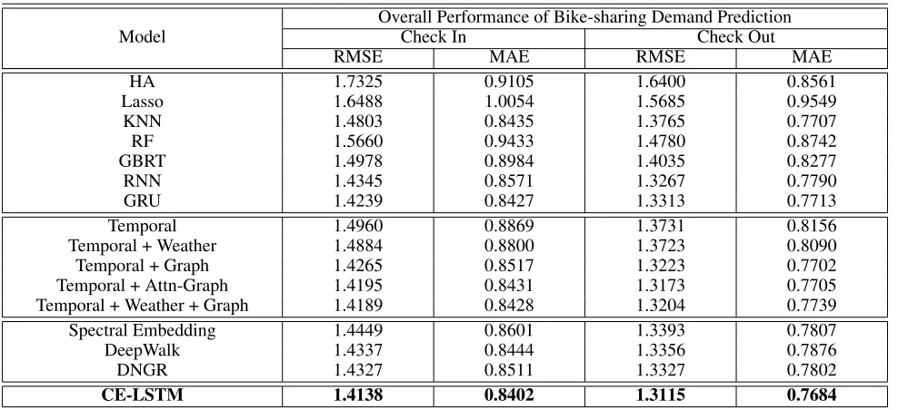
Table 3: Comparison with Different Variants and Baseline Methods
Model
Overall Performance of Bike-sharing Demand Prediction
Check In Check Out
RMSE MAE RMSE MAE
HA 1.7325 0.9105 1.6400 0.8561
Lasso 1.6488 1.0054 1.5685 0.9549
KNN 1.4803 0.8435 1.3765 0.7707
RF 1.5660 0.9433 1.4780 0.8742
GBRT 1.4978 0.8984 1.4035 0.8277
RNN 1.4345 0.8571 1.3267 0.7790
GRU 1.4239 0.8427 1.3313 0.7713
Temporal 1.4960 0.8869 1.3731 0.8156
Temporal + Weather 1.4884 0.8800 1.3723 0.8090
Temporal + Graph 1.4265 0.8517 1.3223 0.7702
Temporal + Attn-Graph 1.4195 0.8431 1.3173 0.7705
Temporal + Weather + Graph 1.4189 0.8428 1.3204 0.7739
Spectral Embedding 1.4449 0.8601 1.3393 0.7807
DeepWalk 1.4337 0.8444 1.3356 0.7876
DNGR 1.4327 0.8511 1.3327 0.7802
CE-LSTM 1.4138 0.8402 1.3115 0.7684
Performance Comparison
Table 3 shows the average performance of the proposed method compared to other baseline competitors. As we can see, the HA perform poorly because only values of previ-ous demands in the the same time of the day are used. Gen-erally, with the collaborative representation learned from multi-source and heterogeneous spatial-temporal data, even the Lasso withl1-norm regularization can improves the
ac-curacy of the prediction. Usually, the collaborative repre-sentations corresponding to similar predicted target values are similar, it makes the K-NN regression training based on distance metrics can achieve considerable performance. Be-sides, GBRT and RF are tree-based methods widely used in time series prediction. The GBRT model, with the charac-teristics of low deviation and high variance with respect to RF, performs better in specific experiments. For deep learn-ing methods which can capture the dependency of correlated relationship within time steps, the CE-LSTM achieved state-of-the-art performance comparing to RNN, GRU and others. We can see that the LSTMs is more conducive to take tempo-ral modeling with collaborative representations learned from multi-source and heterogeneous spatio-temporal data.
Furthermore, we verified the performance of different variants and showed results in Table 3. We can see that LSTMs has a poor performance by only taking the context feature of transition. Meanwhile, the introduction of spatio-temporal graph into spatio-temporal representation can make a greater contribution to the improvement of predictive perfor-mance than weather information. In addition, the experimen-tal results prove that the dynamic attention-based graph em-bedding can outperform graph emem-bedding without attention mechanism significantly. Ultimately, the CE-LSTM, mod-eling by temporal representation, attention-based dynamic graph embedding and weather information, achieved the
best performance. We can draw the conclusion that learning importance-aware vectorization representation by STG2Vec makes it possible to successfully mine the correlations be-tween stations and to further enrich the connotation of col-laborative representation in demand prediction tasks.
Additionally, we use Spectral Embedding, DeepWalk (Perozzi, Al-Rfou, and Skiena 2014) and DNGR (Cao, Lu, and Xu 2016) to learn statical graph embedding for each time step and the representation of nodes can be obtained with the same dimensionsdrespectively. We only replace the dynamic graph node representation learned by STG2Vec with the node vector obtained by the above statical graph embedding methods in CE-LSTM for performance com-parison. Experimental results showed that considering only statical spatial dependence makes a limited improvement if there is a lack of mining the information contained in the evolution of the dynamic graph.
Conclusion
Ackowledgments
This work was jointly sponsored by the National Key Re-search and Development of China (No.2016YFB0800404) and the National Natural Science Foundation of China (No.61572068, No.61532005) and the Fundamental Re-search Funds for the Central Universities of China (No.2018YJS032).
References
Bao, J.; He, T.; Ruan, S.; Li, Y.; and Zheng, Y. 2017. Planning bike lanes based on sharing-bikes’ trajectories. In
Proceedings of the 23rd ACM SIGKDD International Con-ference on Knowledge Discovery and Data Mining, 2017, 1377–1386.
Box, G. E. P., and Pierce, D. 1968. Distribution of resid-ual autocorrelations in autoregressive-integrated moving av-erage time series models.Publications of the American Sta-tistical Association65(332):1509–1526.
Cao, S.; Lu, W.; and Xu, Q. 2016. Deep neural networks for learning graph representations. In Proceedings of the Thirtieth AAAI Conference on Artificial Intelligence, 2016, 1145–1152.
Chen, L.; Zhang, D.; Wang, L.; Yang, D.; Ma, X.; Li, S.; Wu, Z.; Pan, G.; Nguyen, T. M. T.; and Jakubowicz, J. 2016. Dy-namic cluster-based over-demand prediction in bike sharing systems. InUbiComp 2016, 841–852.
Chen, P.; Hsieh, H.; Sigalingging, X. K.; Chen, Y.; and Leu, J. 2017. Prediction of station level demand in a bike sharing system using recurrent neural networks. InVTC 2017, 1–5.
Cho, K.; van Merrienboer, B.; Bahdanau, D.; and Bengio, Y. 2014a. On the properties of neural machine translation: Encoder-decoder approaches. InEMNLP, 103–111. Cho, K.; van Merrienboer, B.; G¨ulc¸ehre, C¸ .; Bahdanau, D.; Bougares, F.; Schwenk, H.; and Bengio, Y. 2014b. Learn-ing phrase representations usLearn-ing RNN encoder-decoder for statistical machine translation. InEMNLP, 1724–1734.
Dai, H.; Dai, B.; and Song, L. 2016. Discriminative embed-dings of latent variable models for structured data. InICML 2016, 2702–2711.
Davoian, K., and Lippe, W. 2007. Time series predic-tion with parallel evolupredic-tionary artificial neural networks. In
ICDM 2007, 10–15.
Drucker, H.; Burges, C. J. C.; Kaufman, L.; Smola, A. J.; and Vapnik, V. 1996. Support vector regression machines. InNIPS, 1996, 155–161.
Goyal, P.; Kamra, N.; He, X.; and Liu, Y. 2018. Dyn-gem: Deep embedding method for dynamic graphs. arXiv: 1805.11273.
Grover, A., and Leskovec, J. 2016. node2vec: Scalable fea-ture learning for networks. InProceedings of the 22nd ACM SIGKDD International Conference on Knowledge Discov-ery and Data Mining, 2016, 855–864.
Guo, C., and Berkhahn, F. 2016. Entity embeddings of cat-egorical variables.arXiv: 1604.06737.
He, T.; Bao, J.; Li, R.; Ruan, S.; Li, Y.; Tian, C.; and Zheng, Y. 2018. Detecting vehicle illegal parking events using shar-ing bikes’ trajectories. In Proceedings of the 24th ACM SIGKDD International Conference on Knowledge Discov-ery & Data Mining, 2018, 340–349.
Hochreiter, S., and Schmidhuber, J. 1997. Long short-term memory.Neural Computation9(8):1735–1780.
Hulot, P.; Aloise, D.; and Jena, S. D. 2018. Towards station-level demand prediction for effective rebalancing in bike-sharing systems. InProceedings of the 24th ACM SIGKDD International Conference on Knowledge Discovery & Data Mining, 2018, 378–386.
Johansson, U.; Bostr¨om, H.; L¨ofstr¨om, T.; and Linusson, H. 2014. Regression conformal prediction with random forests.
Machine Learning97(1-2):155–176.
Le, Q. V., and Mikolov, T. 2014. Distributed representations of sentences and documents. InICML 2014, 1188–1196. Li, X., and Bai, R. 2016. Freight vehicle travel time pre-diction using gradient boosting regression tree. InICMLA 2016, 1010–1015.
Liang, Y.; Ke, S.; Zhang, J.; Yi, X.; and Zheng, Y. 2018. Ge-oman: Multi-level attention networks for geo-sensory time series prediction. InIJCAI 2018, 3428–3434.
Lin, L.; He, Z.; Peeta, S.; and Wen, X. 2017. Predicting station-level hourly demands in a large-scale bike-sharing network: A graph convolutional neural network approach.
arXiv: 1712.04997.
Mikolov, T.; Sutskever, I.; Chen, K.; Corrado, G. S.; and Dean, J. 2013. Distributed representations of words and phrases and their compositionality. In NIPS 2013, 3111– 3119.
Perozzi, B.; Al-Rfou, R.; and Skiena, S. 2014. Deepwalk: online learning of social representations. InThe 20th ACM SIGKDD International Conference on Knowledge Discov-ery and Data Mining, 2014, 701–710.
Rumelhart, D. E.; Hinton, G. E.; and Williams, R. J. 1986. Learning representations by back-propagating errors. Na-ture323(6088):533–536.
Wang, Y., and Chaib-draa, B. 2013. A KNN based kalman filter gaussian process regression. In IJCAI 2013, 1771– 1777.
Yan, Y.; Tao, Y.; Xu, J.; Ren, S.; and Lin, H. 2018. Visual analytics of bike-sharing data based on tensor factorization.
J. Visualization21(3):495–509.
Yao, H.; Wu, F.; Ke, J.; Tang, X.; Jia, Y.; Lu, S.; Gong, P.; Ye, J.; and Li, Z. 2018. Deep multi-view spatial-temporal network for taxi demand prediction. InProceedings of the Thirty-Second AAAI Conference on Artificial Intelligence, 2018, 2588–2595.
Yule, G. U. 1927. On a method of investigating periodicities in disturbed series, with special reference to wolfer’s sunspot numbers.Philosophical Transactions of the Royal Society of London226(226):267–298.