A method of localization
and segmentation of intervertebral discs
in spine MRI based on Gabor filter bank
Xinjian Zhu
1, Xuan He
2, Pin Wang
2, Qinghua He
1, Dandan Gao
1, Jiwei Cheng
3*and Baoming Wu
1*Background
Spinal diseases, such as low-back pain (LBP), are common chronic diseases and are harmful to human health. LBP is a common symptom with considerable social and economic repercussions [1]. LBP is experienced by 25 to 50 % of the adult population in the United States. The healthcare costs for spine pain (mainly for LBP) is increasing every year in the United States [2]. The degeneration of intervertebral discs (IVDs) is the main factor resulting in chronic LBP and disability [3]. Analysis of magnetic resonance imaging (MRI), including disc localization and segmentation, is the main tool to assess
Abstract
Background: Spine magnetic resonance image (MRI) plays a very important role in the diagnosis of various spinal diseases, such as disc degeneration, scoliosis, and osteoporosis. Accurate localization and segmentation of the intervertebral disc (IVD) in spine MRI can help accelerate the diagnosis time and assist in the treatment by providing quantitative parameters. In this paper, a method based on Gabor filter bank is proposed for IVD localization and segmentation.
Methods: First, the structural features of IVDs are extracted using a Gabor filter bank. Second, the Gabor features of spine are calculated and spinal curves are detected. Third, the Gabor feature images (GFI) of IVDs are calculated and adjusted accord-ing to the spinal curves. Fourth, the IVDs are localized by clusteraccord-ing analysis with GFI. Finally, an optimum grayscale-based algorithm with self-adaptive threshold, combined with the localization results and Gabor features of the spine, is performed for IVDs segmentation.
Results: The proposed method is verified by an MRI dataset consisting of 278 IVDs from 37 patients. The accuracy of localization is 98.23 % and the dice similarity index for segmentation evaluation is 0.9237.
Conclusions: The proposed Gabor filter based method is effective for IVD localization and segmentation. It would be useful in computer-aided diagnosis of IVD diseases and computer-assisted spine surgery.
Keywords: Magnetic resonance image, Intervertebral disc, Localization, Segmentation, Gabor filter
Open Access
© 2016 Zhu et al. This article is distributed under the terms of the Creative Commons Attribution 4.0 International License (http:// creativecommons.org/licenses/by/4.0/), which permits unrestricted use, distribution, and reproduction in any medium, provided you give appropriate credit to the original author(s) and the source, provide a link to the Creative Commons license, and indicate if changes were made. The Creative Commons Public Domain Dedication waiver (http://creativecommons.org/publicdomain/ zero/1.0/) applies to the data made available in this article, unless otherwise stated.
RESEARCH
*Correspondence: [email protected]; wbm@ vip.163.com
1 State Key Laboratory
for Trauma, Burn and Combined Injury, Fifth Department, Research Institute of Field Surgery, Daping Hospital, Third Military Medical University of Chinese PLA, Chongqing 400042, China
3 Department
of Orthopaedics, 113th Hospital, Ningbo 315040, Zhejiang, China
degenerative disk disease and evaluate the spinal cord, ligaments, and lesions, as it pro-vides high-resolution, high-contrast images in serial contiguous slices [4].
Previously, disc localization and segmentation in spine MRI was performed by the radiologists manually, and the results depended on the a priori knowledge and experi-ence. Additionally, manual localization and segmentation is laborious and lacks repro-ducibility between observers. Therefore, it is necessary to develop methods to localize and segment the IVDs automatically. An accurate localization and segmentation with computer-aided diagnosis (CAD) for discs in spine MRI would be useful in the quanti-fication of disc degeneration, diagnosis of the disease, and computer-assisted spine sur-gery [5–7]. But, the differences in size, shape, appearance, intensity of different IVDs, and the ambiguous IVD boundaries and similar intensity with surrounding tissues may increase the difficulty of recognition.
Model-based methods are often used to analyze IVDs in past years. Alomari et al. [6] proposed a two-level probabilistic model for localization of discs from MRI. Micho-poulou et al. [7] also presented a semiautomatic approach to segment both normal and degenerated lumbar IVDs. Peng et al. [8] used a model-based searching method to local-ize whole spine discs. Castro et al. [9] segmented the IVDs using active contour models and fuzzy C-means. Haq et al. [10] proposed a segmentation approach based on the dis-crete simplex surface model. Law et al. [11] employed a novel anisotropic-oriented flux model to segment the IVDs. These methods are effective for IVDs with CAD, but need manual operations or user-controlled manners to refine the results.
Many other methods have attracted attention because of their potential implications. Chevrefils et al. [12] used a watershed transform and morphological operations to locate regions containing structures of interest. The drawback of this method is the over-seg-mentation. Neubert et al. [13, 14] proposed an automated approach to extract the 3D segmentations and localization of lumbar and thoracic IVDs using statistical shape anal-ysis and registration of grey level profiles.
Some methods based on machine and deep learning have recently been proposed. Oktay et al. [15] proposed a SVM-based Markov random field method to label the lum-bar discs. However, they only detect six discs with their graphical model and require the existence of both T1 and T2 scans to detect the spinal cord. Ghosh et al. [5, 16] achieved the localization of lumbar discs using histogram of oriented gradients along with SVM. Furthermore, a method is proposed to segment all the tissues simultaneously in a lum-bar sagittal MRI, using an auto-context approach, instead of any explicit shape features or models. It made strong use of heuristics and information from complementary axial scans. Cheng et al. [17] used a machine-learning based technique to localize and seg-ment the 3D IVDs from MRIs. The IVD localization was done by estimating the image displacements from a set of randomly sampled 3D image patches to the IVD center. The IVDs were segmented by classifying image pixels around disc centers as background or foreground. Kelm et al. [18] combined marginal space learning with a generative ana-tomical network to detect and label the IVDs. An optional case-adaptive segmentation approach was proposed to segment the IVDs and vertebrae in MRI and CT, respectively.
distinctly characteristic, relatively regular and similar elliptic structure. The extraction of IVD structure information, such as shape and direction, and avoiding interference from peripheral tissues is challenging. The Gabor filter, a windowed Fourier trans-form, derives from the work of Gabor D. Daugman [19] extended the Gabor filter to two-dimensional (2D) spatial position. Given the biological background and the opti-mal space and spatial-frequency localization of Gabor filter [20], it is widely used for image process applications [21–23]. When the direction and frequency of the objects in an image are consistent with those of 2D-Gabor filters, the wavelet transformation has a strong response. Since the IVDs in spinal MRI are regular and ellipse-shaped, the recog-nition of IVDs is possible by transformation of Gabor filtering.
We propose an unsupervised computer-aided IVD localization and segmentation method based on Gabor filter bank, which does not require any training. Among various wavelet bases, the 2D Gabor filters provide good resolution both in temporal and fre-quency domains, and provide the optimal basis to extract local features because of: (1) Frequency motivation: both multi-resolution and multi-orientation properties of Gabor wavelet are optimal for measuring local spatial frequencies [24]; (2) morphology moti-vation: it distorts the tolerance space for pattern recognition tasks [24]. The proposed method adopts Gabor filters to extract the structural features of IVDs, and localize and segment the IVDs. The information from the Gabor filter is capable of increasing the accuracy and automation degree for IVD localization and segmentation.
Methods
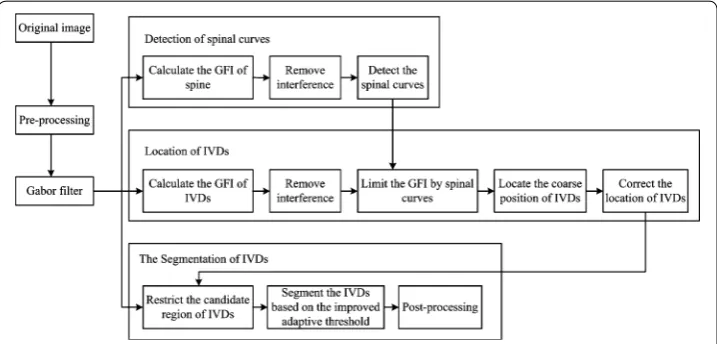
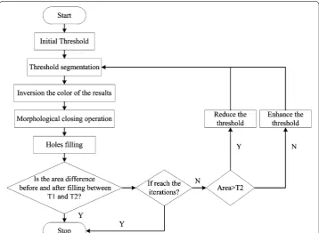
Flow diagram
The flow chart of the proposed method is shown in Fig. 1. It includes the Gabor filter design, detection of spinal curves, localization of IVDs, and segmentation of IVDs. First, a set of 2D-Gabor filters, with different frequencies and directions, are used in image filtering to get a series of Gabor images. Second, Gabor features of the spine are cal-culated and the spinal curves are detected. Third, the Gabor features images (GFI) of IVDs are calculated and limited by spinal curves. Fourth, the IVD localization is per-formed by cluster analysis. Correction of localization is done to improve the accuracy of
localization results. Last, segmentation of IVDs is performed based on the Gabor filter, localization results, and an improved self-adaptive threshold.
Setting of the Gabor filter
Effective extraction of the IVD features depends on the setting of the Gabor kernel func-tion. Due to the elliptic shape of IVDs, the parameter σ of Gabor kernel is different in
horizontal x and vertical y direction. In addition, there is an angle between the IVDs and the horizontal plane. Therefore, the Gabor kernel is defined as [25]:
where, x′=xcosθµ+ysinθµ,y′= −xsinθµ+ycosθµ represent the spatial locations of pixels. In spatial domain, the parameters θµ, ων, and σ represent the direction, wave-length, and Gaussian window of Gabor filter bank, respectively.
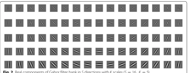
The parameters of Gabor are set as follows: to describe the local features of images, a Gabor filter bank has S directions and K scales (usually S =8, K =5) [20]. However, the
IVDs have a relatively uniform size and the differences among their angles are smaller. A Gabor filter bank in 16 directions with five scales is used. The upper frequency limit
ωmax= π2 is set according to the experience. Since the size of IVDs is relatively uniform, the frequency spacing factor f =√42 is set to obtain the effective center frequency. The effective radius of the Gaussian window is expressed as rv= 2
√ 2σ
ωv . According to the characteristics of the IVD (the width occupies at least 25 pixels and the thickness is about half of the width), σx= ω3kv,σy= ω6kv (where k=
√
2 ln 2). The symmetric Gabor kernel window with the size of 31×31 is used, based on experiment. Gabor filter bank is shown as Fig. 2.
Localization of IVDs
Detection of spinal curves
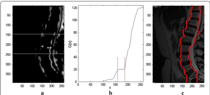
In order to reduce the impact of background on localization and segmentation, the spi-nal edges are detected to narrow the searching range. Since the spispi-nal curves are nearly vertical, the spinal GFI is obtained by subtracting the GFI of horizontal direction from (1)
ψ (x,y,θµ,ων)= 1 2π σxσy
exp
−1
2
x′
σx
2 +
y′
σy
2
+iωνx′
µ=0,. . .,S−1, v=0,. . .,K−1
that of vertical direction. Taking Gv,µ as the Gabor-filtered image with direction µ and scale v, the spinal GFI Gspine can be described as Eq. (2):
where v∈C= {0, 1,. . .,S−1}, µ∈U= {0, 1,. . .,K−1}, U1= {0, 1, 2, 3, 4, 5, 14, 15} , and U2= {7, 8, 9, 10, 11} represent the directions close to the vertical and horizontal
planes, respectively. Obviously, the negative values in Gspine are not the edge information
of spine. Then, the Gspine is processed as Eq. (3).
where G(n) is the sum of the GFI for the first n column (Fig. 3b), and N is the column number of the image. Since the middle of the spine is nearly straight, the p rows in the middle of the MRI images are selected to detect the spinal edges. As shown in Fig. 3b, the curve of G(n) is approximately in the horizontal plane in the middle of the spinal
region (the middle of the two white lines in Fig. 3a). The process include: first, the cent-ers of the left and right spinal edges (the white crosses in Fig. 3a) are obtained by search-ing the crosssearch-ing points for Gspine and center of spine (the white point in Fig. 3a from
center to both sides). Second, the search range is limited between the two white lines in Fig. 3a. Third, the left and right spinal edges are obtained by searching the correspond-ing region from above the centers of left or right spinal edges to both sides, respectively. The Fig. 3c shows the result of spinal edges.
(2) Gspine=
ν∈C,µ∈U1
Gν,µ−
ν∈C,µ∈U2
Gν,µ
(3) Gspine(x,y)=
Gspine(x,y), Gspine(x,y)≥0 0, Gspine(x,y) <0
(4) G(n)=
n
x=1
(M+p)/2
y=(M−p)/2
Gspine(x,y), n=1. . .N
Fig. 3 Detection of spinal curves. a Spinal GFI Gspine The white point is the center of the spine, and the white crosses are the centers of left and right spinal edges. b The sum of the coefficients of the first n columns G(n).
Localization of IVDs
The localization of IVDs is based on GFI information. GFI for localization of IVDs is calculated similar to the process for spines, but the directions of U1 and U2 are differ-ent. According to the anatomical knowledge, the angle between the long axis of the IVD and the horizontal line of MRI is almost ± 30°. Therefore, U1= {7, 8, 9, 10, 11} and
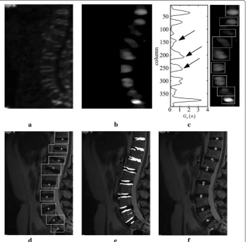
U2= {1, 2, 3, 4, 5} represent directions close to the long axis of IVDs and close to the ver-tical directions, respectively. The IVDs information image GMdisc (Fig. 4b) is obtained by
median filtering (elliptical filter template, long axis: 44 pixels, minor axis: 17 pixels) on the IVDs GFI (Fig. 4a). The searching range of IVDs is narrowed by spinal curves.
The process of localization needs some a priori information. The centroid of the IVD is the locating point. In order to obtain the coordinate value of the locating point
(XIVD,YIVD), two aspects of a priori anatomical knowledge are adopted: I)Abscissa x of
most IVDs is roughly located in the same vertical line, except for the last few ones that lean slightly to the right; II) The offsets of vertical y range from 20 mm to 50 mm (25 pixels to 60 pixels in this study). The information of local maximum of GMdisc, combined
Fig. 4 IVDs localization information based on the Gabor filter. a IVDs GFI. b IVDs information images GMdisc. c
with a priori knowledge, is used for coarse localization. In this process, correction of centre-of-gravity shift is also performed to improve the localization accuracy in case of severe spinal curvature. The process includes:
Step 1: Calculate the horizontal cumulative curve Gh(n) and the candidate vertical
coordinate values. Gh(n) is obtained by adding each row with Eq. (5), Where M
is the number of rows of the image. The coordinates of local maximum values are the candidates.
Step 2: Calculate the coarse YIVD. According to the a priori information II, the closer
points merge into one. The YIVD is achieved after removing the points which do
not meet the a priori information II.
Step 3: Calculate the coarse XIVD. The horizontal coordinate XIVD is calculated by a
process similar to that for YIVD, but the regions of calculation are different.
The mid-values of adjacent two YIVD are taken as boundaries to intercept the
IVD part. The same action is performed as Eq. (6) in columns between the two boundaries. The XIVD is obtained based on the a priori information I.
Step 4: Calculate the boxes of IVDs to correct the coarse(XIVD, YIVD). Based on the
results of Step 3, the rectangular regions of IVDs (Fig. 4d) are found by the boundary of the local peak of Gh(n) (Fig. 4c) and Gv(n). The upwards and
downwards edges of the box in Fig. 4c are calculated by the minimum points and zero points of Gh(n). Then the left and right edges of the box are calculated
by the minimum points and zero points of Gv(n) limited by upwards and
down-wards edges. Figure 4c shows the boxes in GMdisc. Figure 4d shows the boxes in the original image. The angles of IVDs are obtained by analyzing the GFIs information in the rectangular regions.
Step 5: Calculate the accurate center of IVDs (XIVD,YIVD). The binary image of GMdisc
is calculated in the boxes obtained in step 3. Figure 4e shows the superposition of the original image and the binary image. Subsequently, the corrected locali-zation of IVDs is obtained by calculating the centroid of the binary image. As shown in Fig. 4f, the white circles are the final localization results (XIVD,YIVD).
Segmentation of IVDs
Combining the localization results and spinal curves,the segmentation of IVDs is per-formed based on GFIs with an adaptive threshold. The main steps include:
Step 1: Delineate the candidate region of the IVD. The initial candidate region of each IVD for localization is comprised of the spine curves and the rectangular
(5) Gh(n)=
N
x=1
GMdisc(x,n), n=1. . .M
(6) Gv(n)=
M
y=1
GMdisc
regions of IVDs (Fig. 4d). In this region, the average of GFIs of different fre-quencies Gµ¯ is calculated in the direction µ. The maximum Gµ¯ can reflect the
boundary of the IVD. The Gµ¯ in the direction µ with S different frequencies is defined as Eq. (7).
The binary image of maximum Gµ¯ is obtained using the Otsu method. The up
and down boundaries of the candidate region are comprised of the spine curves. The left and right boundaries are comprised of the fitting curve of the outer boundaries of the binary image of maximum Gµ¯ .
Step 2: Calculate the adaptive local threshold TIVD. Due to the ambiguous boundary
and diverse shapes of IVDs, global threshold is not appropriate to segment the IVDs. Therefore, the local threshold (TIVD) of each IVD is adopted to
seg-ment the IVDs. As shown in Fig. 5, TIVD is obtained by self-adaption iteration
and used for segmentation of IVDs. The initial threshold is calculated by the Otsu method. A1 is the difference between the area of candidate region of the
IVD and the area of the binary image of maximum Gµ¯ . A2 is 1/2 area of the
binary image of maximum Gµ¯ . T1 and T2 are min(A1,A2) and max(A1,A2) area, respectively. The number of iterations is 30.
Step 3: Calculate the coarse segmentation of the IVD. The coarse segmentation results of IVDs are used in steps 2 to 5, in Fig. 5, with an adaptive local threshold TIVD.
(7)
¯
Gµ
x,y = 1
S
v∈C
Gν,µ
Step 4: Post-process for IVD segmentation. The coarse segmentation result may con-tain holes, non-smooth areas, and superfluous portions. In order to obcon-tain the accurate segmentation, a morphological operator is used: holes filling, erosion, dilation, and five foreground pixels on the background pixel indicate that the pixel is the foreground pixel. When a segmentation result has many connected regions, the largest region is retained.
Results and discussion
Ethic statement
This study is approved by the Ethics Review Board of the Third Military Medical Univer-sity, Chongqing, China. All records, information, and images were anonymized and de-identified prior to analysis. All patients or their legal representatives signed the written informed consent.
Image acquisition
This dataset was composed of mid-sagittal T2-weighted (T2WI) images from 37 patients with LBP for more than 6 months. In total, 278 IVDs (T11/T12 ~ L5/S1) of MRI images were utilized for validating the proposed localization methods. All MRI images were supplied by Xinqiao Hospital, The Third Military Medical University, China. MRI was performed with a 1.5-T Signa system (General Electric Company, Milwaukee, America), and the parameters of the T2WI were: TR: 3000 ms; TE: 100 ms; FOV: 30 × 30; and number of sagittal sections: 9.
Results of localization
In this study, 278 IVDs of MRI images from 37 patients were utilized to validate the pro-posed method. All methods were implemented in MATLAB R2010b. Of a total of 283 IVDs, 278 IVDs were located by our method, with only five IVDs seen outside of the localization.
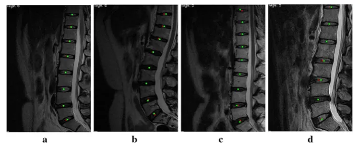
We compared the localization with our method and the manual method. As Fig. 6
shows, the red squares are the results of our method and the green circles are those of the manual method. The four MRIs shown in the Fig. 6a–d contain the typical cases
including normal patient, herniation and IVD degeneration, different intensity and interference, and different spine curvature. These figures show that the results of our method have good agreement with those of the manual operation.
To evaluate the performance of the method quantitatively, localization accuracy Acc
was used. Acc is the percentage of automatic IVD centers which visually lie inside the
IVD. It is defined as:
where DiscAutoTure is the number of correct results of automatic localization of IVDs, DiscAutoTure is the number of all results of automatic localization of IVDs. The results show that a high localization accuracy Acc of 98.23 % could be achieved with the method
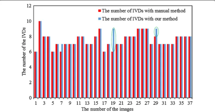
proposed. The comparison between the number of IVDs with our localization method and those with manual method is shown in Fig. 7.
The Euclidean distances between the structure center located by our method and the corresponding manual method were also calculated. Three surgical specialists delineated the contours of each structure manually. Based on the contours, the computer calculated the centers of the IVDs with a snake-based method [26]. The boxplot of the Euclidean distances for the spine structures in 37 images is shown in Fig. 8. The median, top, and bottom lines of the box represent the 50th, 25th, and 75th percentiles, respectively, and the pluses are the statistical outliers. Although there are 14 off-group points from 278 in all cases, these points are all in IVDs and not far from the results of the manual opera-tion. Table 1 shows the average localization error from reference annotation to the local-ized positions.
In order to test the validity of our method in the other dataset, experiments were performed on the publicly available SpineWeb database which is available for public access at http://spineweb.digitalimaginggroup.ca/spineweb. The localization results of SpineWeb database are shown in Fig. 9. Figure 9a–d are from different databases
(8) Acc= DiscAutoTure
DiscAuto ×
100 %
and subjects. The mean and standard deviation of localization using Dataset seven of SpineWeb was 2.60 ± 1.90 mm.
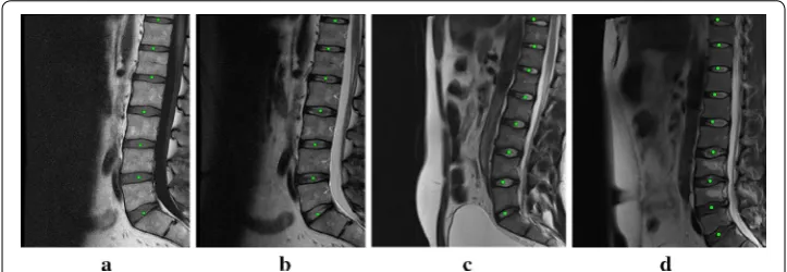
Results of segmentation
The same cases were used to validate the segmentation. Figure 10 shows the segmenta-tion results with our proposed method and manual operasegmenta-tion. The green contours are the results of our method, and the red contours are the results of the manual method. The figure shows that the results of the two methods are highly consistent for normal cases. Figure 10c–d show the results for cases with higher intensity, herniation, and
Fig. 8 Boxplot of the Euclidean distances between the structure center localized with our method and the corresponding manual method for 37 MR images in the dataset
Table 1 Average localization error (in mm) from reference annotation to the localized positions
Disc label Mean ± STD Median Max Min
L5-S1 3.2258 ± 2.0326 3.0415 8.5399 0.7835
L4-L5 2.3505 ± 1.0514 2.0809 6.0460 0.6439
L3-L4 2.0117 ± 1.6307 1.6358 8.3857 0.2093
L2-L3 1.6300 ± 0.9993 1.4974 4.3328 0.2453
L1-L2 1.7608 ± 1.0563 1.5384 5.0205 0.0899
T12-L1 1.5694 ± 0.9160 1.5824 3.7216 0.1191
T11-T12 1.8817 ± 1.0163 1.7635 4.1179 0.3896
T10-T11 2.4007 ± 2.6023 1.5336 10.2740 0.3162
T9-T10 2.5622 ± 2.2372 1.3515 6.0186 0.5505
T8-T9 12.3583 – – –
IVD degeneration. As shown in Fig. 10b, in cases with more serious curvature and IVD degeneration, L2-L3 are over-segmented and L3-L4 are slightly under-segmented. Although the spinal curves were deviated, overall segmentation results of IVDs were satisfactory.
To evaluate the performance of the segmentation method quantitatively, Sensitivity (Sen), Specificity (Spe), and Dice Similarity Index (DSI) were calculated [12–15]. The Sen ,
Spe, and DSI were defined as:
where M is the area of the manually segmented IVD, A is the area of the segmented IVD experimentally, and I is the MRI image.
(9)
Sen= M∩A
M
(10)
Spe= I−M∪A I−M
(11)
DSI= 2|M∩A| |M| + |A|
Fig. 9 The localization results of the SpineWeb database. a, b and c, d are from different databases and subjects
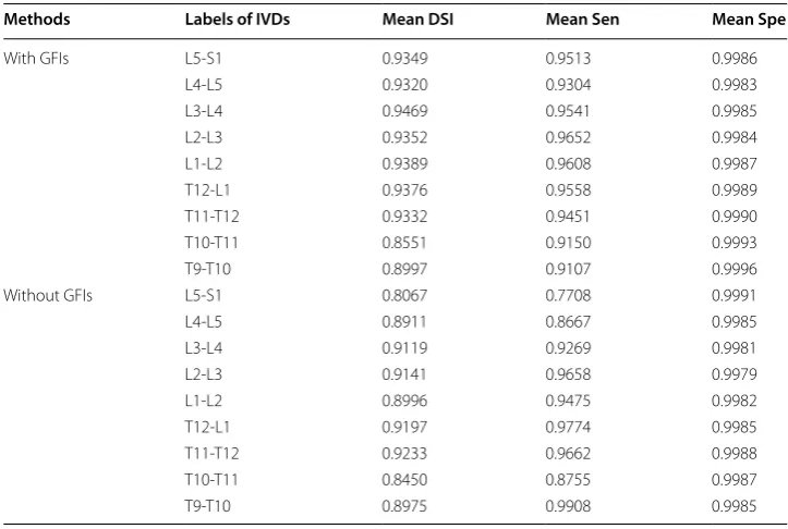
The index analysis of 37 MRIs is shown in Table 2. The overall average values of the DSI with and without GFIs is 0.9237 and 0.8899, respectively. The index values show that the results with GFIs restriction have significant improvements compared with those without GFIs restriction. The results of the proposed method have good agree-ment with those of the manual segagree-mentation. There was reduced probability of over- or under-segmentation.
Discussion and conclusion
The proposed method achieves high accuracy without the need of user interaction, tech-nologist point, or coronal or axial slices. This benefit comes from the shape-recognition ability of the method based on Gabor filter bank. GFIs reduce the localization error by extracting the target information correctly, and correction operation reduces the impact of inaccurate IVD localization by taking all candidate points into account. In the seg-mentation part, the adaptive threshold based on the GFI is proposed. The GFI limits the candidate regions, which improves the accuracy of the segmentation results.
The localization and segmentation of the proposed method takes almost 10 s (the manual segmentation with a snake-based method [26] takes almost 5 min). Eight sec-onds are required for one image to complete the localization process, and only 2 s are required to complete the segmentation part. The main contribution to the computation time is by wavelet transformation (about 7.5 s). With the development of computer tech-nology, our method is likely to satisfy the requirements of real-time clinical application.
The Gabor filter bank makes use of the direction and morphology of the IVDs. Due to the interference in direction and morphology in some MRIs, few IVDs were localized outside of the localization results. The results were not significantly affected by the extra localization because recognition techniques, such as areas and morphology, were added to the segmentation method. However, the localization accuracy is likely to increase
Table 2 The comparison of DSI, Sen, and Spe with and without GFIs
Methods Labels of IVDs Mean DSI Mean Sen Mean Spe
With GFIs L5-S1 0.9349 0.9513 0.9986
L4-L5 0.9320 0.9304 0.9983
L3-L4 0.9469 0.9541 0.9985
L2-L3 0.9352 0.9652 0.9984
L1-L2 0.9389 0.9608 0.9987
T12-L1 0.9376 0.9558 0.9989
T11-T12 0.9332 0.9451 0.9990
T10-T11 0.8551 0.9150 0.9993
T9-T10 0.8997 0.9107 0.9996
Without GFIs L5-S1 0.8067 0.7708 0.9991
L4-L5 0.8911 0.8667 0.9985
L3-L4 0.9119 0.9269 0.9981
L2-L3 0.9141 0.9658 0.9979
L1-L2 0.8996 0.9475 0.9982
T12-L1 0.9197 0.9774 0.9985
T11-T12 0.9233 0.9662 0.9988
T10-T11 0.8450 0.8755 0.9987
even further with the use of the texture feature in this method. This method was verified with 278 IVDs from 37 patients. Further verification and improvement of the method is warranted in future studies. Additional studies with large sample sizes are necessary to use GFIs for exploring the characters of IVDs and segmentation. We plan to carry out more studies with large sample sizes. Further work also includes classifying the degree of IVD degeneration using the segmentation and curvature results. Additionally, the GFI information will be used to detect curvature of spines more accurately so diseases of the spine can be accurately diagnosed.
In conclusion, we proposed a localization and segmentation method for IVDs based on Gabor wavelet. In contrast to traditional methods, Gabor filtering for shape-repre-sentation is proposed. The results and quantitative evaluation show that this method has a high accuracy compared with manual operation. It does not need supervision or train-ing with large datasets before use. Therefore, this method will be useful in computer-aided diagnosis of the disease and computer-assisted spine surgery.
Authors’ contributions
XZ proposed the original concept of the method and draft the manuscript; XH and PW performed the statistical analysis and helped to draft the manuscript; QH and DG analyzed the parameters for the study; BW and JC gave the theoreti-cal guidance and condition support, and are the corresponding authors; All authors read and approved the final manuscript.
Author details
1 State Key Laboratory for Trauma, Burn and Combined Injury, Fifth Department, Research Institute of Field Surgery,
Daping Hospital, Third Military Medical University of Chinese PLA, Chongqing 400042, China. 2 College of
Communica-tion Engineering, Chongqing University, Chongqing 400044, China. 3 Department of Orthopaedics, 113th Hospital,
Ningbo 315040, Zhejiang, China. Acknowledgements
This research is funded by the National Natural Science Foundation of China under Grant No. 11304382, 61108086, and the Third Military University Science Foundation under Grant No. 2012XJQ23, and the Project of State Key Laboratory of Trauma, Burns and Combined Injury of China under Grant No. SKLZZ(II)201403.
Competing interests
The authors declare that they have no competing interests.
Received: 17 November 2015 Accepted: 14 March 2016
References
1. Ract I, Meadeb JM, Mercy G, Cueff F, Husson JL, Guillin R. A review of the value of MRI signs in low back pain. Diagn Interv Imaging. 2015;96:239–49.
2. Dagenais S, Galloway EK, Roffey DM. A systematic review of diagnostic imaging use for low back pain in the United States. Spine J. 2014;14:1036–48.
3. Lzzo R, Popolizio T, D’Aprile P, Muto M. Spinal pain. Eur J Radiol. 2015;84(5):746–56.
4. Siemund R, Thurnher M, Sundgren PC. How to image patients with spine pain. Eur J Radiol. 2015;84:757–64. 5. Ghosh S, Malgireddy MR, Chaudhary V, Dhillon G. A new approach to automatic disc localization in clinical lumbar
MRI: combining machine learning with heuristics. 9th IEEE International Symposium on Biomedical Imaging (ISBI). 2012;114–117.
6. Alomari RS, Corso JJ, Chaudhary V. Labeling of lumbar discs using both pixel-and object-level features with a two-level probabilistic model. IEEE Trans Med Imaging. 2011;30:1–10.
7. Michopoulou SK, Costaridou L, Panagiotopoulos E, Speller R, Panayiotakis G, Todd-Pokropek A. Atlas-based segmentation of degenerated lumbar intervertebral discs from MR images of the spine. IEEE Trans Biomed Eng. 2009;56:2225–31.
8. Peng ZG, Zhong J, Wee W, Lee JH. Automated vertebra detection and segmentation from the whole spine MR images. 2005 27th Annual International Conference of the IEEE Engineering in Medicine and Biology Society. 2005;2527–2530.
9. Castro-Mateos I, Pozo JM, Lazary A, Frangi AF. 2D segmentation of intervertebral discs and its degree of degenera-tion from T2-weighted magnetic resonance images. Medical imaging 2014. Comput Aided Diagn. 2014;9035:17. 10. Haq R, Aras R, Besachio DA, Borgie RC, Audette MA. 3D lumbar spine intervertebral disc segmentation and
compres-sion simulation from MRI using shape-aware models. Int J Comput Assist Radiol Surg. 2015;10:45–54.
• We accept pre-submission inquiries
• Our selector tool helps you to find the most relevant journal • We provide round the clock customer support
• Convenient online submission • Thorough peer review
• Inclusion in PubMed and all major indexing services • Maximum visibility for your research
Submit your manuscript at www.biomedcentral.com/submit
Submit your next manuscript to BioMed Central
and we will help you at every step:
12. Chevrefils C, Cheriet F, Grimard G, Aubin C. Watershed segmentation of intervertebral disk and spinal canal from MRI images. Image Anal Recognit. 2007;4633:1017–27.
13. Neubert A, Fripp J, Engstrom C, Schwarz R, Lauer L, Salvado O, et al. Automated detection, 3D segmentation and analysis of high resolution spine MR images using statistical shape models. Phys Med Biol. 2012;57:8357–76. 14. Neubert A, Fripp J, Engstrom C, Walker D, Weber MA, Schwarz R, et al. Three-dimensional morphological and signal
intensity features for detection of intervertebral disc degeneration from magnetic resonance images. J Am Med Inform Assoc. 2013;20:1082–90.
15. Oktay AB, Akgul YS. Simultaneous localization of lumbar vertebrae and intervertebral discs with SVM-based MRF. IEEE Trans Biomed Eng. 2013;60:2375–83.
16. Ghosh S, Chaudhary V. Supervised methods for detection and segmentation of tissues in clinical lumbar MRI. Com-put Med Imaging Graph. 2014;38:639–49.
17. Chen C, Belavy D, Yu W, Chu C, Armbrecht G, Bansmann M, Felsenberg D, Zheng G. Localization and segmentation of 3D intervertebral discs in MR Images by data driven estimation. IEEE Trans Med Imaging. 2015;34:1719–29. 18. Kelm BM, Wels M, Zhou SK, Seifert S, Suehling M, Zheng Y, Comaniciu D. Spine detection in CT and MR using
iter-ated marginal space learning. Med Image Anal. 2012;17:1283–92.
19. Daugman JG. Uncertainty relation for resolution in space, spatial frequency, and orientation optimized by two-dimensional visual cortical filters. J Opt Soc Am. 1985;2:1160–9.
20. Daugman JG. Complete discrete 2-D Gabor transforms by neural networks for image analysis and compression. Transact Acoust Speech Signal Process. 1988;36:1169–79.
21. Radman A, Jumari K, Zainal N. Iris segmentation in visible wavelength images using circular gabor filters and optimi-zation. Arab J Foren Eng. 2014;39:3039–49.
22. Hacihaliloglu I, Rasoulian A, Rohling RN, et al. Local phase tensor features for 3-D ultrasound to statistical shape + pose spine model registration. IEEE Trans Med Imaging. 2014;33:2167–79.
23. Shu T, Zhang B. Non-invasive health status detection system using gabor filters based on facial block texture fea-tures. J Med Syst. 2015;39:1–8.
24. Ji P, Jin L, Li X. Vision-based vehicle type classification using partial Gabor filter bank. 2007 IEEE International Confer-ence on Automation and Logistics. 2007;1037–1040.
25. Lee TS. Image representation using 2D Gabor wavelets. IEEE Trans Pattern Anal Mach Intell. 1996;18:959–71. 26. Zhu X, Zhang P, Shao J, et al. A snake-based method for segmentation of intravascular ultrasound images and its