T E C H N I C A L A D V A N C E
Open Access
Using the Beta distribution in group-based
trajectory models
Jonathan Elmer
1, Bobby L. Jones
2and Daniel S. Nagin
3*Abstract
Background:We demonstrate an application of Group-Based Trajectory Modeling (GBTM) based on the beta distribution. It is offered as an alternative to the normal distribution for modeling continuous longitudinal data that are poorly fit by the normal distribution even with censoring. The primary advantage of the beta distribution is the flexibility of the shape of the density function.
Methods:GBTM is a specialized application of finite mixture modeling designed to identify clusters of individuals who follow similar trajectories. Like all finite mixture models, GBTM requires that the distribution of the data composing the mixture be specified. To our knowledge this is the first demonstration of the use of the beta distribution in GBTM. A case study of a beta-based GBTM analyzes data on the neurological activity of comatose cardiac arrest patients.
Results:The case study shows that the summary measure of neurological activity, the suppression ratio, is not well fit by the normal distribution but due to the flexibility of the shape of the beta density function, the distribution of the suppression ratio by trajectory appears to be well matched by the estimated beta distribution by group. Conclusions:The addition of the beta distribution to the already available distributional alternatives in software for estimating GBTM is a valuable augmentation to extant distributional alternatives.
Keywords:Group-based trajectory modeling, Beta distribution, Cardiac arrest
Background
A trajectory describes the evolution of a behavior, biomarker, or some other repeated measure of interest over time. Group-based trajectory modeling (GBTM) [1], also called growth mixture modeling [2], is a special-ized application of finite mixture modeling designed to identify clusters of individuals who follow similar trajec-tories. Originally developed to study the developmental course of criminal behavior [3], GBTM is now widely applied in biomedical research in such diverse applica-tion domains as chronic kidney disease progression [4], obesity [5,6], pain [7], smoking [8], medication adoption and adherence [9,10], and concussion symptoms [11].
Like all finite mixture models, GBTM requires that the distribution of the data composing the mixture be specified, although there are no theoretical limits on the distributions that could be used. In GBTM, parameters
of the specified distribution (e.g. mean and variance of a normal distribution) are allowed to vary across trajectory groups. To our knowledge, previously published applica-tions have all specified the normal distribution, perhaps with censoring, the Poisson distribution, perhaps with zero-inflation, or the binary logit function. Real-world continuous biomedical data are frequently not normally distributed even after allowing censoring. This is par-ticularly true of biomarker data, which are generally positive, right skewed, and often zero-inflated. This creates a need for flexible alternatives to the Gaussian distribution [12].
In this article, we demonstrate an application of GBTM based on the beta distribution. It is offered as an alternative to the normal distribution for modeling con-tinuous longitudinal data are poorly fit by other distribu-tions. The primary advantage of the beta distribution is the flexibility of the shape of the density function. The normal density function, even in its censored form, must follow some portion of it familiar bell-shaped form * Correspondence:[email protected]
3Heinz College, Carnegie Mellon University, Pittsburgh, PA 15206, USA
Full list of author information is available at the end of the article
whereas the shape of beta distribution is far less constrained. The disadvantage of beta distribution is that the data under study must be transformable to a 0–1 scale.
Methods
The beta distribution can be parameterized in several different ways. One which is particularly useful for our purposes was proposed by [12]. Let y denote a beta distributed random variable:
P yð ;μ;ϕÞ ¼Γð ÞμϕΓΓð Þϕ
1−μ
ð Þϕ
ð Þyμϕ−1
where 0 < y < 1, 0 < μ < 1 and ϕ > 0. Under this parameterization E(y) = μ and Var(y) =μ(1−μ)/1 +ϕ). The parameter ϕ is known as the precision parameter, because for anyμa larger value ofϕresults in a smaller Var(y).
We turn now to incorporating the beta distribution into GBTM. In describing a GBTM, we denote the distribution of trajectories by P(Yi), where the random vector Yi=(yi1,yi1,…yiT) represents individual i’s longitu-dinal sequence of measurements over T measurement occasions. The GBTM assumes that the population distribution of trajectories arises from a finite mixture composed ofJgroups. The likelihood for each individual i, conditional on the number of groupsJ, may be written as:
P Yð Þ ¼i
XJ
j¼1
πj∙P Y ijj;θj ð1Þ
where πj is the probability of membership in group j, and the conditional distribution ofYigiven membership in j is indexed by the unknown parameter vector θj. Typically, the trajectory is modeled by a polynomial function of time (or age). For the case where P(Yi|j;θj) is assumed to follow the beta distribution, its mean at time t for group j,μjt, is linked to time as follows:
μjt ¼β0jþβ1jtþβ2jt2…:
where, in principle, the polynomial can be of any order.1 Note that the parameters linking μjt to time are trajec-tory group specific, thus allowing the shapes of trajector-ies to vary freely across group. Also associated with each trajectory group is a group specific precision parameter,
ϕj. The remaining components of θj pertain to the parameterization ofπj, which in this case is specified to follow a multinomial logistic function.
For given j, conditional independence is assumed. In other words, except as explained by individual i’s trajectory group membership, serial observations in the
random vectorYiare assumed to be independent of one another. Thus, we may write:
Pk Yijj;βj
¼YT
t¼1
pk yit;j;βj
ð2Þ
While conditional independence is assumed at the level of the latent trajectory group, at the population level outcomes are not conditionally independent because they depend on a latent construct, trajectory group membership. See chapter 2 of [1] for a discussion of the conditional independence assumption.
The GBTM modeling framework does not require that the random vector Yi be complete for all individ-uals. For the baseline GBTM specified above, missing values in Yi are assumed missing at random. However, for applications such as that described below where measurement ends due to some external event—in this case due to the death of the patient or the patient awakening from coma—an extension of GBTM described in [13] may be used to account for non-random dropout.
Detailed discussion of the methods to approach selec-tion of J, the number of latent groups in the populaselec-tion, and the order of the polynomial specifying each group’s trajectory are beyond the scope of this paper and have been previously described [1]. Briefly, no test statistics identifies the number of components in a finite mixture [14, 15]. Also, as argued in [1], in most application do-mains of GBTM the population is not literally composed of a finite mixture of groups. Instead the finite mixture is intended to approximate an underlying unknown continuous distribution of trajectories for the purpose of identifying and summarizing its salient features. As de-scribed in [14,16], finite mixture models are a valuable tool for approximating an unknown continuous distribu-tion. In this paradigm, model selection is performed by combining test statistics such as AIC and BIC, which can guide the statistician to identify which model best fits the data. This is combined with expert knowledge of which model best reveals distinctive trajectory groups that are substantively interesting. The order of the polynomial used to model each group’s trajectory is typically determined by starting with an assumed maximum order for each trajectory group then suc-cessively reducing the order if the highest order term is statistically insignificant.
Results
We demonstrate use of the beta distribution in a GBTM of data quantifying brain activity of 396 comatose pa-tients resuscitated from cardiac arrest. The University of Pittsburgh Institutional Review Board approved all as-pects of this study. The data result from an observa-tional cohort study of consecutive comatose patients hospitalized at a single academic center from April 2010 to October 2014 that underwent continuous electroen-cephalographic (EEG) monitoring for at least 6 h after resuscitation from cardiac arrest. Not included are patients that arrested from trauma or catastrophic neurological event, and those who awakened, died or were transitioned to comfort care within 6 h of hospital arrival.
The point of departure for our demonstration is prior work that applied GBTM to an indicator of brain activity, suppression ratio, a quantitative measure of the proportion of a given EEG epoch that is suppressed below a particular voltage threshold for activity [19]. In the first hours after cardiac arrest, many patients’ EEGs are quite suppressed (50–80%) [19] showed that patients with persistently low or rapidly improving suppression ratios often make good recoveries, while persistent suppression over the first 36 h is ominous.
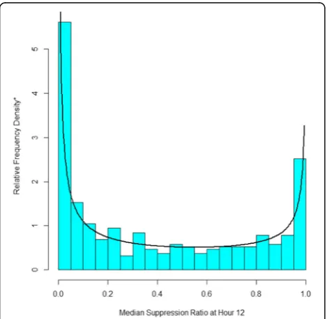
Our main concern with the prior application was the assumption that suppression ratio followed a censored normal distribution with a minimum of 0 and a max-imum of 1. To illustrate the basis for our concern, con-sider Fig. 1, which reports a histogram of the median
suppression ratio at hour 12. It has two spikes close to the minimum of 0 and the maximum of 1. In between, the suppression ratio is approximately uniformly distrib-uted. The histogram bears no resemblance to the normal distribution. While it is possible for a mixture of cen-sored normal distributions to approximate the histogram in Fig. 1, the distribution of suppression ratio data within the four groups reported in [19] does not resem-ble the normal distribution. By contrast, overlying the histogram is a beta distribution with μ= 0.42 and ϕ= 0.77, which closely resembles the observed distribution of the suppression ratio.
Figure 2 shows a three group, beta-based trajectory model over the first 48 h of suppression ratio measure-ments.2
Because EEG monitoring may be ended either because the patient dies or awakens, the model accounted for non-random subject attrition as described in [13]. The three group model was selected because it optimized both BIC and AIC compared to fewer groups, and models with four or more groups were sometimes unstable and did not identity additional trajectory groups that were clinically interesting in terms of their survival prospects. For the three group model, group 1 is specified to follow a cubic function of time, and groups 2 and 3 are specified to follow quadratic functions of time because as discuss above the cubic term of these trajectories were statistically insignificant at the .05 level. As was found in the prior analysis based on the censored normal assumption, trajectory group is strongly associ-ated with survival probability. Overall, only about a third of patients survive to hospital discharge. However, survival probability for group 3, which accounts for an estimated 32.0% of patients who have a persistently high suppression ratio, only an estimated 2.3% survive. By contrast group 1, which accounts for an estimated 26.8%
Fig. 1The Distribution of Hour 12 Suppression Ratio Data with the
Best Fitting Beta Distribution. *The sum of the heights of the relative frequency density bars multiplied by their width sum to 1.0 so as to conform the with estimated beta density
Fig. 2Three Group Trajectory Model with Beta Distributed
of patients, follows a persistently low suppression ratio trajectory. For this group survival probability is an estimated 69.8%. In between are group 2 patients.
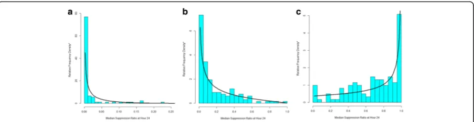
How well do these beta distribution-based trajectories fit the data? Fig. 3overlays the actual distribution of the suppression ratio data by trajectory group with the predicted distribution according to the beta distribution at hour 24. Inspection of the Figure reveals that for each trajectory group the actual and predicted values nicely correspond even though across trajectory group the distribution of the suppression ratio are quite different. Trajectory group 1 (Fig. 3a) and trajectory group 2 (Fig. 3b) have right skewed suppression ratio distribu-tions, whereas the distribution for trajectory group 3 (Fig. 3c) is left skewed. Moreover, the left skew of groups 1 and 2 are distinctly different, with group 1’s skew far more extreme than group 2’s. The fit between the actual and predicted data distribution by trajectory group is similarly good for other hours.
Discussion
We note that the use of the beta distribution does re-quire an adjustment for boundary observations, namely data equal to 0 or 1, which are formally not feasible for a beta distributed random variable. For boundary obser-vations we follow the suggestion of [20] and add/sub-tract from 0/1 data points a small amount equal to .5 divided by the number of subjects, 396. However, a use-ful generalization to avoid this ad hoc adjustment would be the addition of the equivalent of the zero-inflation factor in the Poisson distribution to account for data at the boundary values of the beta distribution.
Conclusion
We have demonstrated an extension of GBTM that adds the beta distribution to the heretofore usually applied distributions for modeling trajectories—the censored normal, zero-inflated Poisson, and binary logit. The beta option provides an alternative to the censored normal distribution for modeling continuous or approximately
continuous measured outcomes measured over age or time. Figure 1 makes clear that the normal distribution poorly fits the suppression ratio data whereas the beta distribution provides a far better fit. Figure3 also makes clear that due to the flexibility of the beta distribution a beta-based GBTM can accommodate differences in the distribution of the suppression ratio across trajectory group and over time that are not readily accommodated by the normal distribution.
Endnotes
1
Up to 5th order polynomials can be estimated in the software used to estimate the models reported in the case study.
2
The call to the Stata-based trajectory estimation used to estimate this model was as follows:traj, var.(srt1-srt48) indep(t1-t48) model(beta) order(3 2 2) dropout(0 0 0) where srt* is the median supression ratio at hour * and t* is the hour of measurement from 1 to 48 and the“ drop-out”component of the call activates the generalization of GBTM to account for nonrandom subject attrition.
Abbreviations
EEG:Electroencephalography; GBTM: Group-based trajectory modeling; ML: Machine learning; PPGM: Posterior probability of group membership; SR: Suppression ratio
Acknowledgements
Support for this research was provided by the Center for Machine Learning and Health, Carnegie Mellon University. Dr. Elmer’s research time is supported by the NIH through grant 5K23NS097629.
Availability of data and materials
The datasets used and/or analyzed during the current study are available from the corresponding author on reasonable request.
Authors’contributions
JE, BLJ and DSN each made substantial contributions to the conception and design of the work, jointly performed analysis of the data, have given approval for its publication and take responsibility for the work. JE was responsible for data acquisition. DSN and JE drafted the manuscript, and BLJ provided critical revisions of important intellectual content. All authors read and approved the final manuscript.
Ethics approval and consent to participate
The University of Pittsburgh Institutional Review Board approved all aspects of this study. Consent to participate is not applicable.
Consent for publication
Not applicable.
Competing interests
The authors declare that they have no competing interests.
Publisher’s Note
Springer Nature remains neutral with regard to jurisdictional claims in published maps and institutional affiliations.
Author details
1
Department of Emergency Medicine, Critical Care Medicine and Neurology, University of Pittsburgh, Pittsburgh, PA, USA.2University of Pittsburgh
Medical Center, Pittsburgh, PA, USA.3Heinz College, Carnegie Mellon University, Pittsburgh, PA 15206, USA.
Received: 9 October 2018 Accepted: 15 November 2018
References
1. Nagin D. Group-based modeling of development. Cambridge, Mass: Harvard University Press; 2005.
2. Muthen B. Latent Variable Analysis. In: SAGE Handbook of Quantitative Methodology for the Social Sciences. D. Kaplan (ed.). Thousand Oaks: SAGE Publications, Inc.; 2004. pp 345.
3. NAGIN DS, LAND KC. Age, criminal careers, and population heterogeneity: specification and estimation of a nonparametric, mixed poisson model*. Criminology. 1993;31:327–62.
4. Burckhardt P, Nagin DS, Padman R. Multi-trajectory models of chronic kidney disease progression. AMIA Annu Symp Proc. 2016;2016:1737–46. 5. Malhotra R, Ostbye T, Riley CM, Finkelstein EA. Young adult weight
trajectories through midlife by body mass category. Obesity (Silver Spring). 2013;21:1923–34.
6. Reinders I, Murphy RA, Martin KR, Brouwer IA, Visser M, White DK, Newman AB, Houston DK, Kanaya AM, Nagin DS, Harris TB, Health A, Body Composition S. Body mass index trajectories in relation to change in lean mass and physical function: the health, Aging and Body Composition Study. J Am Geriatr Soc. 2015;63:1615–21.
7. Nicholls E, Thomas E, van der Windt DA, Croft PR, Peat G. Pain trajectory groups in persons with, or at high risk of, knee osteoarthritis: findings from the knee clinical assessment study and the osteoarthritis initiative. Osteoarthr Cartil. 2014;22:2041–50.
8. Lessov-Schlaggar CN, Kristjansson SD, Bucholz KK, Heath AC, Madden PA. Genetic influences on developmental smoking trajectories. Addiction. 2012;107:1696–704.
9. Lo-Ciganic WH, Gellad WF, Huskamp HA, Choudhry NK, Chang CC, Zhang R, Jones BL, Guclu H, Richards-Shubik S, Donohue JM. Who were the early adopters of dabigatran?: an application of group-based trajectory models. Med Care. 2016;54:725–32.
10. Juarez DT, Williams AE, Chen C, Daida YG, Tanaka SK, Trinacty CM, Vogt TM. Factors affecting medication adherence trajectories for patients with heart failure. Am J Manag Care. 2015;21:e197–205.
11. Yeates KO, Taylor HG, Rusin J, Bangert B, Dietrich A, Nuss K, Wright M, Nagin DS, Jones BL. Longitudinal trajectories of postconcussive symptoms in children with mild traumatic brain injuries and their relationship to acute clinical status. Pediatrics. 2009;123:735–43.
12. Ferrari S, Cribari-Neto F. Beta regression for modelling rates and proportions. J Appl Stat. 2004;31:799–815.
13. Haviland AM, Jones BL, Nagin DS. Group-based trajectory modeling extended to account for nonrandom participant attrition. Sociol Methods Res. 2011;40:367–90.
14. Everitt B, Hand DJ. Finite mixture distributions. London ; New York: Chapman and Hall; 1981.
15. Titterington DM, AFM S, Makov UE. Statistical analysis of finite mixture distributions. Chichester; New York: Wiley; 1985.
16. Heckman J, Singer B. A method for minimizing the impact of distributional assumptions in econometric models for duration data. Econometrica. 1984;52:271–320.
17. Dennis JEG, M D, Walsh RE. An adaptive nonlinear least-squares algorithm. AMC Trans Math Softw. 1981;7:348–68.
18. Dennis JE, Mei HHW. Two new unconstrained optimization algorithms which use function and gradient values. J Optim Theory Appl. 1979;28:453–82.
19. Elmer J, Gianakas JJ, Rittenberger JC, Baldwin ME, Faro J, Plummer C, Shutter LA, Wassel CL, Callaway CW, Fabio A, Pittsburgh Post-Cardiac Arrest S. Group-based trajectory modeling of suppression ratio after cardiac arrest. Neurocrit Care. 2016;25:415–23.