METHODOLOGY
Model errors in tree biomass estimates
computed with an approximation to a missing
covariance matrix
Steen Magnussen
1*and Oswaldo Ismael Carillo Negrete
2Abstract
Background: Biomass and carbon estimation has become a priority in national and regional forest inventories. Biomass of individual trees is estimated using biomass equations. A covariance matrix for the parameters in a bio-mass equation is needed for the computation of an estimate of the model error in a tree level estimate of biobio-mass. Unfortunately, many biomass equations do not provide key statistics for a direct estimation of model errors. This study proposes three new procedures for recovering missing statistics from available estimates of a coefficient of deter-mination and sample size. They are complementary to a recently published study using a computationally intensive Monte Carlo approach.
Results: Our recovery approach use survey data from the population targeted for an estimation of tree biomass. Examples from Germany and Mexico illustrate and validate the methods. Applications with biomass estimation and robust recovered fit statistics gave reasonable estimates of model errors in tree level estimates of biomass.
Conclusions: It is good practice to provide estimates of uncertainty to any model-dependent estimate of above ground biomass. When a direct approach to estimate uncertainty is impossible due to missing model statistics, the proposed robust procedure is a first step to good practice. Our recommended approach offers protection against inflated estimates of precision.
Keywords: Linear regression, Nonlinear regression, Weighted regression, Residual variance, Robust estimation, Parametric bootstrap
© 2015 Magnussen and Carillo Negrete. This article is distributed under the terms of the Creative Commons Attribution 4.0
International License (http://creativecommons.org/licenses/by/4.0/), which permits unrestricted use, distribution, and
reproduc-tion in any medium, provided you give appropriate credit to the original author(s) and the source, provide a link to the Creative Commons license, and indicate if changes were made.
Background
The importance of forest biomass for the global car-bon cycle is widely recognized [1–4]. The imperative of maintaining global levels of forest biomass and slowing regional rates of decline [5] has fostered international cooperation, initiatives, and projects to this end [6–8].
A large number of countries have agreed to implement an accounting system for forest carbon and to report on national-level annual gains and losses [9–11].
With few exceptions, the forest carbon accounting sys-tem has a national forest inventory at its core, and a suite of models to expand and transform inventory data to
forest carbon [12–14]. Carbon components not fully cov-ered by an inventory are typically estimated from activity data (e.g. harvest, disturbance, and erosion) and mod-els fitted to data from research studies of, for examples: litter-fall; litter-decomposition; fine-root turnover; seed production; and dead and downed-woody debris.
An estimate of the uncertainty in a carbon balance has become a routine requirement [15, 16]. When the core inventory data comes from a probability sample, the uncertainty arises from three sources: observational and measurement errors [17–19], sampling errors, and errors in model parameters [12, 20]. The live above-ground for-est tree biomass (AGB) accounts for the largfor-est contribu-tion to the forest carbon balance [21, 22].
In situ determination of AGB is extremely costly and destructive. A model‒dependent approach with
Open Access
*Correspondence: [email protected]
1 Natural Resources Canada, 506 West Burnside Road, Victoria, BC V8Z 1M5, Canada
prediction of biomass from a biomass equation, with easy-to-measure explanatory variables, is the only practi-cally feasible alternative [21, 23].
The development of a complete set of regional, species- and stratum-specific biomass models constitutes a heavy financial outlay that cannot be met in many parts of the world. As a substitute for models fitted to local data, an analyst may decide to use the most suitable off-the-shelf biomass equation [21, 23–36].
It is, of course, very difficult to ascertain whether an off-the-shelf model is suitable for a particular application or not [37]. It remains a risky proposition to use exter-nally fitted models without any form of validation or re-calibration to local conditions [38]. An adopted model generates the desired predictions of above-ground bio-mass but a valid estimate of the associated covariance of model-parameters is needed to compute an estimate of the uncertainty in a prediction [12, 39, p. 73, 40]. A model-bias can only be quantified in a validation with actual observations of above-ground biomass and the predictors in a model [41, pp. 172 and 232, 42].
Although we have a plethora of equations for above-ground biomass as a function of, for example, stem diam-eter at a reference height of 1.3 m above ground level [21, 26, 31, 43], information regarding the covariance matrix of model parameters is often missing. Available fit statis-tic is generally limited to one or more of the following: standard errors of estimated parameters, the coefficient of determination, the standard deviation of lack-of-fit residuals, and sample size [44].
This study demonstrates methods for recovering a covariance matrix for model parameters in a biomass equation from fit statistics restricted to: sample size (n) and the coefficient of determination (R2) [44]. Our non-use of a possibly available estimate of the standard deviation of empirical residuals rests with its sensitivity to outliers [45], a strong dependency on the sampling design [39, p. 55], the distribution of the response and explanatory variables in the study that gave us the equa-tion of interest. Wayson et al. [44] proposed a Monte-Carlo approach to recover missing estimates of the covariance among parameters in a biomass equation. The key idea in their approach is to generate a distribu-tion of pseudo-data that mirrors, to the extent possible, a known or assumed distribution of explanatory vari-ables in the sample trees behind an equation. The tenet behind our approach is different. It is rooted in survey sampling [39]. Hence, the recovered estimates of uncer-tainty are assumed compatible with estimates that could have been obtained from a sample taken from the popu-lation, for which we desire estimates of biomass. It is fully recognized that our recovery is neither perfect nor unbi-ased. However, supported by our results, we argue that
our approach is consistent with the main objective of any recovery procedure: to estimate model errors in popula-tion estimates of biomass as opposed to a rediscovery of ‘lost’ estimates of model errors.
Our demonstrations include examples with equations and data from the first German national forest inventory in 1987 (BWI-1) [40, 46] and the 2004–2009 Mexican National Forest Inventory [47–49]. We discuss limita-tions to our approach, and recommend a robust recovery method. We also emphasize the need to develop new and fully documented biomass equations for important spe-cies in regions where they are currently lacking.
Results
Examples from Germany
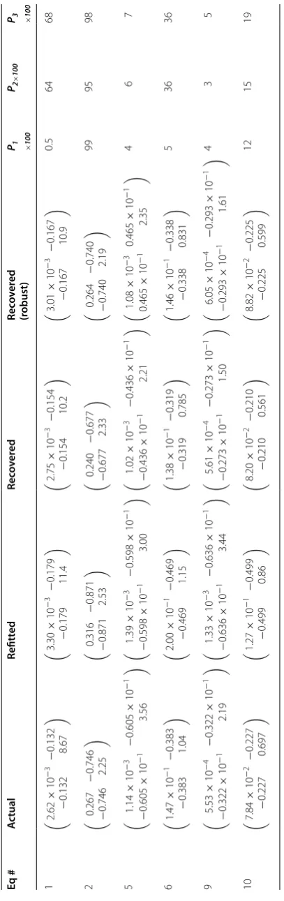
Substitutes for missing covariance matrices for the bio-mass models in Table 1 are listed in Table 2. For refitted matrices, there were three rejections of the null hypoth-esis of equality (actual = refitted) at the 5 % level of sig-nificance. For the recovered matrices there were one rejection, and for the robust recovery there were zero rejections. A distinct pattern emerged when compar-ing refitted, recovered, and robust variances. Refittcompar-ing appears to overestimate the variance in a regression parameter; by approximately 70 % for the first param-eter and approximately 35 % for the second paramparam-eter. In contrast, the recovered variances were, on average, smaller than the actual variances (5 and 16 %, respec-tively). Robust estimates of variance were closer to actual estimates of variance than refitted and recovered esti-mates. Substitute covariance matrices for the nonlinear models were, in general, closer to the missing (actual) covariance matrix than a substitute covariance matrix for a linear model.
Taking into consideration that the relative error in the regression coefficient to diameter DBH or DBH2 is six to twelve times smaller than the relative error in the regres-sion coefficient to √DBH×HT or√HT, a bias in the former is much more serious than in the latter. For un-weighted linear and nonlinear equations, the robust pro-cedure appears as the most attractive. As well, the strong impact of errors in the first regression coefficient on a tree-level estimate of AGB amplifies concerns surround-ing the overestimation of model-errors encountered with the refitting procedure.
(two rejections of the null hypothesis of no difference). Yet there is an average overestimation of the first variance by 23 % and an average underestimation of the second by 25 %. Considering the larger contribution to the model error variance from the former, the overestimation is a concern. A robustly recovered matrix was in four cases significantly different from the actual covariance matrix and overestimated variances by 72 and 24 %.
Recovering an estimate of the residual variance was, as expected, easier than recovering a covariance matrix. The relative error in recovered estimates of the residual standard error varied from approximately −20 to +35 %.
Two of eight estimates were significantly different from the actual values (F-ratio test, P = 0.02), for the remain-ing six, the level of significance was 0.10 or greater.
Attempts at a recovery of the covariance matrices for the generalized above-ground biomass Eqs. 13–15 in Table 1 [26] failed, regardless of method. With the recov-ery methods, the estimated standard deviations of the three regression parameters were 2–8 times greater than those listed in Table 3 of Muukkonen [26]. Had we used the tabled values of the root mean squared error in lieu of the recovered substitute, the estimated errors would have been approximately 30–70 times too small. The failure is easy to explain: the fit-statistics of the generalized model apply to the set of models that are generalized. Footnotes to Table 3 in Muukkonen [26] carefully explain the con-strained interpretation of the table entries. Due to the poor accuracy of the recovered generalized covariance matrices they were not used to gauge the error-propaga-tion to estimates of tree-level AGB.
All recovery procedures are fraught with numerical problems due to co-linearity among regression coeffi-cients (correlations coefficoeffi-cients varied between −0.87 and −0.97), and large differences in accuracy of param-eter estimates. For example, the matrix condition num-ber varied between 14.1 and 14.9, and determinants were less than 10−5 suggesting a serious potential of amplified estimation errors when inverting a covariance matrix [50, 51]. Challenges of this nature will also be encountered in applications of the proposed procedures.
A summary of the effect of replacing a missing (actual) covariance matrix with a substitute approximation on the model-error in an estimate of the mean per tree AGB (kg) is provided in Table 4. With the un-weighted linear mod-els the relative model error in the average tree-level esti-mate of AGB is 7–12 % (column ACT in Table 4). Model errors in estimates based on a nonlinear un-weighted equation were approximately 2–3 % points lower.
Weighted regressions were uniformly superior with the lowest relative errors. Results with the substitute covari-ance matrices followed—by and large—these trends with estimates within one to 6 % points from results with the actual estimate of covariance. In the case of weighted regressions: two poor results with the refitting procedure with PINE data, and two for the robust recovery with BEECH data, stands out as examples of inflated estimates of model-error. The remaining estimates of error appear reasonable; yet do not indicate that one recovery proce-dure is substantially and consistently better than the pre-sented alternatives.
Examples from Mexico
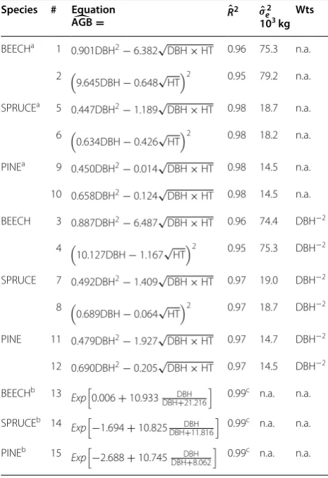
For Guazuma ulmifolia and Ochroma pyramidale the substitute estimates of the parameter error variances Table 1 Species group above-ground forest tree biomass
(AGB kg tree−1) equations
Sample size is 50 trees per species group.
a BWI-1987 Predictions of AGB times a uniformly distributed random error
[0.9,1.1] fitted to DBH (mm) and HT (dm).
b Generalized AGB equations from Table 8 (Temperate zone) in Muukkonen P
and Heiskanen J [76]. DBH is in centimeters (cm).
c Amount of variation in predicted AGB values captured by the generalized
equation.
Data were selected from 335 plots from the 1987 (West) German national forest inventory (BWI-1987). Plots were dominated by one of the three species
groups. Selected trees have a DBH ≥ 7 cm, and were selected with a probability
proportional to their basal area at breast height (basal area factor of 4), [77, ch. 8]. Species # Equation
AGB=
ˆ R2 σˆ2
e
103 kg Wts
BEECHa 1
0.901DBH2−6.382√DBH×HT 0.96 75.3 n.a.
2
9.645DBH−0.648√HT2 0.95 79.2 n.a.
SPRUCEa 5
0.447DBH2−1.189√DBH×HT 0.98 18.7 n.a.
6
0.634DBH−0.426√HT2 0.98 18.2 n.a.
PINEa 9
0.450DBH2−0.014√DBH×HT 0.98 14.5 n.a.
10 0.658DBH2−0.124√DBH×HT 0.98 14.5 n.a.
BEECH 3 0.887DBH2−6.487√DBH×HT 0.96 74.4 DBH−2
4
10.127DBH−1.167√HT
2 0.95 75.3 DBH−2
SPRUCE 7 0.492DBH2−1.409√DBH×HT 0.97 19.0 DBH−2
8
0.689DBH−0.064√HT2 0.97 18.7 DBH−
2
PINE 11 0.479DBH2−1.927√DBH×HT 0.97 14.7 DBH−2
12 0.690DBH2
−0.205√DBH×HT 0.97 14.5 DBH−2
BEECHb 13
Exp0.006+10.933DBH+21.216DBH 0.99c n.a. n.a.
SPRUCEb 14
Exp−1.694+10.825DBHDBH+11.816 0.99c n.a. n.a.
PINEb 15
Table 2 A ctual , r efitt ed , and r ec ov er ed c ov arianc e ma tric es of non-w eigh ted r egr ession c oefficien ts in equa tions Ac tual c ov ar ianc e ma tr ic es ar
e based on a sample siz
e of 50.
Pi
(
i
=
1, 2, 3) is the pr
obabilit
y under
H0
of
: (1) ac
tual
=
refitt
ed; (2) ac
tual
=
rec
ov
er
ed; (3) ac
tual = robust . S ee T able 1 for r ef er enc e t o equa tion number ing . Eq # A ctual Refitt ed Rec ov er ed Rec ov er ed (r obust)
P1 ×100
P2×
100
P3 ×100
Table 3 A ctual , r efitt ed , and r ec ov er ed c ov arianc e ma tric es of r egr ession c oefficien ts in w eigh
ted least squar
es equa tions in Table 1 Ac tual c ov ar ianc e ma tr ic es ar
e based on a sample siz
e of 50.
Pi
(
i
=
1, 2, 3) is the pr
obabilit
y under
H0
of
: (1) ac
tual
=
refitt
ed; (2) ac
tual
=
rec
ov
er
ed; (3) ac
tual = robust . Eq. # A ctual Refitt ed Rec ov er ed Rec ov er ed (r obust)
P1 ×100
P2 ×100
P3 ×100
were, not statistically significant from the actual esti-mates of error (Table 5). This is spite of overestimating, by a factor of approximately two, the variances in the regression parameters for G. ulmifolia. The relative small sample sizes of 18 and 16 trees limit our power to declare practically important differences significant. In case of Inga vera and Trichospernum mexicanum the substitute variances were two to four times larger than the pub-lished estimates. Each recovery procedure led to inflated estimates of variance. The basic recovery method holds a slight edge over the other two. We did not attempt a weighting scheme in the recovery procedure as the log transformation of AGB and DBH in most cases remove variance heteroscedasticity in the original scale of the residuals. Power functions as used for Quercus spp. are extremely sensitive to the weighting schemes used in the German examples. Besides, the original biomass equa-tions were not obtained by weighted least squares [52] so we did not employ a weighted recovery scheme.
Substitute estimates of the residual standard error were considerably and statistically significantly smaller (30– 240 %) than the published values. These results paired with the inflation of the variance of regression coeffi-cients suggest a much smaller variation of the explana-tory variables in the samples from the national invenexplana-tory than in the sample used for fitting. A uniform distribu-tion of the explanatory variables in the model fitting sam-ple [53] could explain our results.
Tabled estimates of the residual standard errors for the three Quercus spp. Were three to four times smaller than recovered estimates. We noted that even a small reduc-tion of 1–2 % in the published value of Rˆ2 would bring the two sets of estimates within approximately 20 % of each other. Power functions are notorious in this regard.
When the uncertainty in biomass equation parameters was propagated to tree-level estimate of AGB, we obtained the average relative per tree model-errors in Table 6. Over-all, the relative model errors in the average per tree AGB in Table 4 Relative model errors (%) in estimates of the mean per tree above-ground tree biomass with actual (ACT), refit-ted (REFIT), recovered (RECOV), and robustly recovered (RREC) covariance matrices for the parameters in the biomass equations in Table 1
Species Model Weights? ACT REFIT RECOV RREC
BEECH LIN No 11.5 14.0 12.3 12.8
NLIN No 8.7 9.1 8.0 8.4
LIN Yes 4.7 8.8 7.8 11.6
NLIN Yes 4.4 6.6 6.9 9.4
SPRUCE LIN No 9.8 8.4 7.2 7.4
NLIN No 7.0 6.6 5.4 5.6
LIN Yes 6.2 10.0 5.4 7.4
NLIN Yes 5.6 8.5 4.8 6.6
PINE LIN No 6.9 5.9 4.9 5.1
NLIN No 5.3 4.7 3.8 4.0
LIN Yes 4.8 22.3 3.5 4.3
NLIN Yes 4.2 19.0 3.0 3.8
Table 5 Actual, refitted, and recovered variances of regression coefficients in Eqs. 1–7 in Table 8
Actual covariance matrices are based on sample sizes listed in Table 8. Pi (i = 1, 2, 3) is the probability under H0 of: (1) actual = refitted; (2) actual = recovered; (3)
actual = robust.
Eq
# Actual Refitted Recovered Recovered(robust) P×1100
P2
×100
P3
×100
1 (0.04, 0.01) (0.08, 0.01) (0.07, 0.01) (0.10, 0.02) 56 74 49
2 (0.55, 0.42, 0.020) (2.64, 1.39, 0.044) (2.36, 1.25, 0.039) (2.88, 1.52, 0.048) 0.2 0.1 0.1
3 (0.27, 0.048) (0.29, 0.041) (0.26, 0.039) (0.35, 0.053) 99 98 96
4 (0.084, 0.017) (0.33, 0.049) (0.29, 0.043) (0.37, 0.06) 2 5 1
5 n.a. (0.32, 7.1)10−3 (0.20, 9.4)10−3 (0.23, 10.6)10−3 n.a. n.a. n.a.
6 n.a. (0.61, 4.7)10−1 (0.42, 32.2)10−2 (0.12, 9.0)10−1 n.a. n.a. n.a.
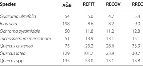
G. ulmifolia appears too low, despite an apparent overesti-mation of the errors in the model parameters. Refitting of a missing covariance matrix via the parametric bootstrap-ping generated unrealistic large estimates of relative errors in Quercus laeta and Quercus spp. Numerical instability of the covariance matrix, small sample sizes, and random multiplicative residuals with a large variance is a recipe for poor results. As expected, the robust recovery produces the largest estimates of relative errors.
Discussion
The need for forest biomass equations has increased sharply over the past decades in response to efforts directed at quantifying stock and stock-changes in for-est carbon and the potential for bioenergy extraction [21, 42, 54]. Ideally there would be an equation for each tree species and region with distinct growth forms and management regimes [55, 56]. We are still far from this ideal. Even the equations we have are generally based on very limited sampling within a relatively small area and range of tree sizes [21]. This is understandable in light of the high costs of producing a biomass equation [21, 26, 57]. Biomass estimates for large trees are therefore fraught with problems of applicability of available bio-mass equations.
In the computation of forest biomass in a large region, country, or even a continent, it is common practice to use a suitable biomass equation for a particular species and growth region [58–60]. In most cases, there is no sepa-rate calibration of chosen biomass equations.
On this background, national and regional estimates of above-ground biomass should be regarded as no more than first-order approximations [16]. The require-ment [11] to quantify or at least assess uncertainty in a national or regional estimate of forest biomass has pre-cipitated a need for estimates of errors in the parameters of employed biomass equations. For a large number of
equations, this information is partially or entirely missing [31, 44].
In a context of model-dependent estimation of for-est tree biomass and model-errors in these for-estimates, a covariance matrix of the model parameters is needed [12, 40]. When this statistic is missing a substitute is needed. Wayson et al. [44] proposed a computationally intensive method for generating a large number of pseudo data of the dependent and independent variables in a biomass equation. Samples are then drawn repeatedly and the model is refitted each time. The sampling aims at mim-icking the actual sampling process (if known) of the origi-nal data behind a biomass equation.
Our proposed procedures for computing a substitute for a missing covariance matrix are computationally faster and make direct use of data of the explanatory variables sampled from the population targeted for an estimation of biomass. The distribution of the explanatory variables used to compute (recover) a covariance matrix plays a pivotal role in both approaches. If the actual distribution behind an equation differs from the distribution in the recovery process, a covariance matrix different from the actual (but unknown) will emerge from a recovery proce-dure. We saw several examples of this in our examples, but an equal number of examples where a substitute matrix was not statistically different from the target matrix. Way-son et al. [44] do not report at this level of details, but we surmise that they encountered similar issues. It is now a question of whether these differences are relevant or not. We argue, that sampling the explanatory variables from the target population vouch for estimates adapted to the application domain rather than to a small sample of trees with unknown representation in the target population.
The most intuitive approach to recover a missing covariance matrix is a variant of the parametric bootstrap [61]. In the textbook version of a parametric bootstrap, n pseudo observations of Y are generated a large number of times (say B) by adding a random draw from the observed empirical regression residuals to the n model predictions obtained from the original regression model and the observed explanatory variables. The regression model is then refitted B times to the pseudo observations of Y. At the end, the analyst has B replications of the covariance matrix of the model parameters. Without observed resid-uals, this approach is not feasible. Instead, our recovery by refitting resorted to random sampling of the explana-tory variables from the target population for biomass estimation, and residuals from a distribution deemed realistic to the case at hand (e.g. a gamma distribution for multiplicative residuals). Although this method in many cases was as good as with alternative approaches, it was equally clear that it entails a considerable risk of poor results. A risk traced to random interactions between Table 6 Estimates of mean AGB kg tree−1 and relative
errors (%) in estimates in mean AGB for seven Mexican species
Estimates are based on tree data provided by the Mexican NFI (see Table 9). The errors are derived with refitted (REFIT), recovered (RECOV), and robustly recovered (RREC) covariance matrices for the parameters in the biomass equations in Table 8.
Species AGBˆ REFIT RECOV RREC
Guazuma ulmifolia 54 5.0 4.7 5.4
Inga vera 198 8.6 8.2 9.0
Ochroma pyramidale 50 11.8 11.2 12.8
Trichospernum mexicanum 51 13.9 13.1 15.1
Quercus castenea 75 23.2 28.6 33.9
Quercus latea 129 101.7 23.9 30.7
residuals and the explanatory variables. For that reason we do not recommend a recovery by model refitting with simulated residuals.
The examples from Germany confirmed that in pres-ence of heteroscedasticity in the model residuals, a weighting with the inverse to the presumed residual vari-ance can be effective [62, ch. 2.11, 63, ch. 2.1]. To carry this efficiency through to a recovered covariance matrix, a weighting scheme applied to the original biomass equa-tion should be replicated in a recovery procedure.
A matrix recovery based on the average (vector) gradi-ent of the model parameters with respect to the explana-tory variables was, in the balance, better suited for the purpose of estimation of model errors in tree-level bio-mass estimates. A robust variant of the recovery is easy to compute and—despite expected and observed larger esti-mates of model-errors—we recommend this procedure as a prudent choice. For the purpose of reasonable estimates model-errors in tree-level estimates of biomass, it is not a strict requirement that a recovered covariance matrix is close to the actual but missing matrix. Most of our estimates, but especially those obtained with the robust recovery procedure, seem reasonable [13, 16, 20, 57, 64]. Our resampling of explanatory variables from inventory data representing the population targeted for an estima-tion of biomass, ensures that the mean of the explanatory variables will be close to the mean in the target popula-tion. Ceteris paribus, this will counter the aforementioned inflation of model-parameter variances [39, ch. 5.4].
An attempt to recover a covariance matrix can end in failure. A failure was demonstrated with the general-ized biomass equations for beech, pine, and spruce in the temperate zone [26, Table 1]. A failure is pre-ordained when estimates of R2 and a root mean squared errors are incompatible with the biomass equation applied to actual data. Our experience should raise awareness of potential pitfalls in published fit-statistics for a generalized equa-tion, unless they reflect a proper meta-analysis [65].
Throughout we have treated published fit statistics as known entities. It would have been preferable to con-sider an empirical Bayesian recovery procedure [66]. The coefficient of determination is pivotal in our proposed procedures. Its sampling variance can only be estimated from the data supporting a biomass equation [67]. To recognize sampling variance in R2, a recovery is repeated a large number of times, each with a random draw from an anticipated distribution of R2, to create an empirical Bayes posterior distribution of the recovered statistic. The recovery procedure by Wayson et al. [44] contains elements of a Bayesian approach.
Although a recovered covariance matrix affords an esti-mate of the model error in a tree level biomass estiesti-mate, the model-error is conditional on a correctly specified model.
If a published biomass equation is the result of an intensive model and variable screening process, we must expect opti-mism in published statistics and model-bias [68].
We have demonstrated the recovery of a missing covari-ance matrix without too much concern about sample size. Clearly, a biomass equation derived from a small sample size has a relatively high risk of model bias due to a high influence of individual observations [62, p. 170]. It is not possible to give a definite recommendation about the mini-mum sample size for our robust recovery procedure. How-ever, a first approximation can be gained from the following example: If we have fitted a linear regression model with three parameters, and we wish to declare a standardized regression residual of 3 as significant at the 5 % level (an indication that the model is unduly influenced by residuals of this magnitude), we need a sample size of approximately 55 [69]. Thus an application of our recovery procedure for regression models supported by less than 55 trees should proceed with caution and attention to robustness.
In large sample inventories the model errors in point estimates of biomass will often dominate sampling errors [12, 40]. Fortunately, when estimating a temporal change in biomass and carbon stock between two inventories, model errors in a difference all but cancel [Ibid]. Thus applying recovered conservative (robust) estimates of a missing covariance matrix will have little impact on the estimate of model errors in a difference.
We have demonstrated that reasonable (robust) esti-mates of model-errors in estiesti-mates of tree-level biomass can be derived from a minimum of two available fit sta-tistics for a biomass equation: the coefficient of deter-mination, and sample size. To complete an estimation of model-errors an analyst need access to forest inventory sample data of the explanatory variables from the popula-tion targeted for biomass estimapopula-tion.
Conclusions
It is good practice to provide estimates of uncertainty to any model-dependent estimate of above ground bio-mass. When a direct approach to estimate uncertainty is impossible due to missing model statistics, the proposed robust procedure is a first step to good practice. Our rec-ommended approach offers protection against inflated estimates of precision.
Methods
The biomass model
The model we consider for above-ground live tree bio-mass is parametric and can be expressed as
where yi is the above-ground forest tree biomass (AGB in kg) of the ith tree, f is a known function (linear or
(1)
nonlinear), xi is a p × 1 row vector of regressor vari-ables including an intercept (if any), b is a q × 1 vector of model parameters, and ei is a residual error. For a linear model p = q.
A model f fitted to n observations of xi and yi(i = 1,…, n) allows a prediction of the expected biomass in the, say, jth tree
ˆ
yj
from knowledge of xj and the estimated parameters bˆ. In the application context of a forest inven-tory (survey) the model in (1) is used to predict AGB for out-of-sample trees. An estimator of the approximate out-of-sample model error variance in an estimate of AGB for a tree j with a known (measured) vector xj of explanatory variables is [70, ch. 6.3]
where σˆe2 is an estimate of the variance of lack-of-fit residuals (ei) of the trees used to fit the model in (1), and
∂f (xj|b)∂−1b is the vector of derivatives (gradients) with respect to the model parameters, and covˆ
ˆ b
is an esti-mate of the covariance among model parameters. All gradients are evaluated at the least squares estimate of b. A superscript ‘t’ denotes the transpose of a vector or a matrix. When the model is linear in b the derivatives in 2 reduces to the vector x.
The q × q covariance matrix for bˆ is [63, p. 17]
The estimation problem
It is clear from (2) that we cannot estimate the error in an out-of-sample estimate of the AGB in a single tree unless we have reasonable estimates of σˆe2 and covˆ bˆ. Note, when we wish to estimate the error in an average of AGB in a large number (m) of trees, the contribution to the error from the residual variance can be ignored as it declines at a rate of m−1, the second term, however, is only averaged over m [62, pp. 28–30].
When we are tasked with estimating the error vari-ance in (2) but do not have estimates of σˆe2 or covˆ
ˆ b
we have to recover reasonable substitutes. Equations (2) and (3) implicitly suggest how to obtain substitutes
˜
σe2 for σˆe2 and cov
ˆ b
for cov
ˆ b
when we at least know the sample size n used to estimate the parameters in the biomass model in (1), and the coefficient of determina-tion Rˆ2 or, preferably, the adjusted coefficient of deter-mination [62, p. 91].
(2)
ˆ
VAGBˆ j= ˆσe2+ ∂f
xj|b
∂b
t
ˆ
covbˆ∂f
xj|b
∂b
(3)
covˆ (b)= ˆσ2
e
ˆ
FtFˆ−
1
with Fˆ =
∂f(x1|b) ∂b ,. . .,
∂f(xi|b) ∂b ,. . .,
∂f(xn|b) ∂b
t
Recovery of missing fit statistics
A basic recovery of a substitute for cov
ˆ b
begins with B random samples (without replacement) of size n of x taken from an inventory sample from the population for which tree-level predictions of AGB via (1) are desired. For each of the B samples, one first computes
where V(zj) denotes the variance of zj =f
xb,j| ˆb
, and ˆ
R2 is a known estimate of the coefficient of determina-tion. Then covb
ˆ b
,b=1,. . .,B is estimated as in (3).
The average over the B replications of σ˜e2 and c ovbˆ
now serves to approximate the error variance in AGB of a sin-gle tree (see (2)). Implicit in this estimator of residual var-iance is the assumption of a homogenous error-structure. It is clear from (4) that the estimate σ˜e2 depends on the sampling distribution of fxb,j| ˆb
which may be quite dif-ferent from the distribution in the original sample used in model fitting. Most biomass functions are fitted to an approximate uniform distribution of the explanatory vari-ables, as it achieves large-sample optimality for model fit-ting [39, ch. 7.5]. However, for typically small sample sizes in biomass studies, this no longer holds. Our repeated sampling from the target population assuage more robust and realistic estimates of the desired covariance matrix. Albeit under the proviso that the reported coefficient of determination has not been maximized by a combination of model- and variable-selection procedures, and a sam-pling design that C. paribus favors a linear model.
Recovery via refitting
A recovered estimate of the residual variance (see (4)) can be used in a parametric bootstrap [71] to recover a substitute for a missing covariance matrix c
ovbˆ
. The refitting begins with n random draws of residuals (ej*, j = 1, …, n) from a t-distribution with n − q degrees of freedom. Pseudo data y∗j =fxj| ˆb
+e∗j is then used to re-estimate the parameters b∗ˆ and the associated covari-ance matrix cov(b∗). This process is repeated B times; the mean of the covariance matrices is now the substitute to use in computing an error of AGB via (2).
Adding a random residual to a biomass prediction yˆj can make yj* negative in violation of AGB ≥ 0. Should that occur we recommend computing yj* from ˆyj×ej∗ where ej* is a random draw from a gamma distribution with parameters ν and ν−1 (i.e. with mean 1.0 and variance ν−1). The parameter ν can be found by using Goodman’s formula for the exact variance of V
ˆ
yie∗i
[72]. However,
(4) ˜
σe2,b=V
f
xb,j| ˆb
×Rˆ−2−1
,
in our examples this formula did not give us real-valued solutions of ν. By solving the equation in [5] for ν we obtained a good first-order approximation.
Recovery of off‑diagonal elements in covbˆ
In some cases estimates of errors in bˆ are available, but without estimates of covariance. In this scenario a substi-tute covariance matrix can be recovered from
Robust recovery
A recovered substitute c ov
ˆ
b may differ substantially from the target covariance matrix cov
ˆ b
when the dis-tribution of xj in the samples taken from the population targeted for a prediction of AGB differs from the distri-bution of xi in the original—but unknown—sample used for model-fitting [39, ch. 5.4]. To mitigate this prospect, we propose a robust recovery of cov
ˆ b
. It is borrowed from Gallant AR [63] and given in (7)
where e˜i is a random draw from a t-distribution with
⌊0.5n⌋ degrees of freedom and variance σ˜e2. The choice of degrees of freedom for the t-distribution is arbitrary; it reflects the fact that most sample sizes supporting a tree biomass model are in the range of 6–30 [21]. A halving of these sample sizes results in increases of 3–21 % in 95 % percentiles from a student’s t-distribution. Robust alter-natives to the correlation coefficients in [6] can be com-puted with a weighting of gradients proportional to the inverse of abs(˜ei).
A weighted recovery
In regressions with a positively valued dependent vari-able (y), it is not uncommon to observe an increase in the variance of regression residuals with an increase in y [73, ch. 5.1]. A weighted least squares (WLS) approach to model-fitting would be appropriate. If f (xi; b) was fitted using WLS the recovery of a substitute for covˆ bˆ should also employ a weighting scheme. Equation [8] provides an example.
(5)
V
ˆ yie∗i
=V
ˆ yi
+ν−1
¯ˆ y2+V
ˆ yi
(6)
cov
ˆ
bk,bˆl�=k
=corr
∂f
xj|b
∂bk
,∂f
xj|b
∂bl
b≡ ˆb
×var(bk)var(bl), k,l=1,. . .,q
(7)
covrobust
ˆ b
=
ˆ
FtFˆ
−1
×
n
i=1 ˜
e2i
∂f(xi|b)
∂b
∂f(xi|b)
∂b
t
b≡ ˆb
ˆ
FtFˆ−
1
where W is an n × n diagonal matrix of sum-to-one weights w1, …, wn. In tree biomass models, the weights would typically be proportional to the inverse of, say, DBHj2 which gives the following weights wj = TDBH2 × DBHj−2 where TDBH2 is the sum of DBHj2 over the n trees. A robust alternative to [8] is obtained by a straightforward extension of [7].
A weighting scheme is also needed when trees for model-fitting were selected by an unequal probability selection scheme. Weights should then be proportional to the inverse of the sample inclusion probability [73, p. 41].
The number B of resampling replications
The value of B was determined adaptively by monitor-ing the Monte Carlo error as a function of B [74]. In our examples we fixed B to 800. With this value of B, the Monte Carlo error in the determinant of c
ovbˆ was less than 4 %.
Comparing recovered and actual covariance matrices A recovered substitute for a covariance matrix may vary considerably from an unknown target estimate when the joint distribution of the explanatory variables in the sample used for fitting differs from the joint-distri-bution in the target population for model application. In our demonstrations we knew, in most cases, the actual estimates of the missing covariance matrix. It is therefore of interest to test the hypothesis of equality between a recovered substitute and the actual estimate. We use Box’s M-test to obtain a Chi square test-statistic and the probability of this test statistic under the null hypothesis of no difference [75, p. 281]. The same test was applied in examples where only the covariance in bˆ are unknown.
Applications
Examples from Germany
We demonstrate the above recovery procedures with 15 biomass equations (Table 1) and data (HT, DBH) from 335 plots in the first German national forest inventory (BWI-1987). Note, the data represent trees selected with probability proportional to their basal area. Their mean HT and DBH are therefore larger than the mean of trees selected with equal probability. However, for purpose of a demonstration, this fact is deemed unimportant.
There are four equations (linear, nonlinear, weighted, un-weighted) for each of three species (BEECH, PINE, SPRUCE). Each equation (no. 1–12) were derived from
(8)
c
ovwtbˆ= ˆσ2 e
ˆ FtWFˆ−
a sample size of n = 50 randomly selected trees from five BWI plots. The five plots were excluded from any recovery procedure. In the model fitting, BWI predic-tions of tree AGB (kg per tree) multiplied with a random uniformly distributed error on the interval [0.9, 1.1] were used as the dependent variable and diameter at a reference height of 1.3 m (DBH) and tree height (HT) were used as predictors. A summary of the BWI data is in Table 7. The remaining three biomass equations
(no. 13–15) are generalized species specific AGB equa-tions from Muukkonen and Heiskanen [76]. They are assumed applicable throughout the temperate zone. An analyst may prefer a generalized biomass equation over a local/regional model derived from a relatively small sample size and potentially from a sub-population with a different relationship between AGB and the explana-tory variables than in a population targeted for estima-tion of AGB.
Examples from Mexico
Four linear (on a log–log scale) biomass equations [53] with published estimates of Rˆ2adj, σˆe, and standard errors of the regression coefficients are used to demonstrate the recovery procedures. The equations (no. 1–4) are in Table 8. Three non-linear biomass equations for Quercus spp. [52] with unknown standard errors of the regression coefficients were also included (no. 5–7).
The recovery procedures are demonstrated with data from the 2004–2009 Mexican national forest inventory [47, 48]. Specifically, 132 sample plots and 1,843 trees with known DBH and HT were included (Table 9). Table 7 Means of DBH, HT, and AGB of trees from the 1987
German National Inventory used in this study
Standard deviations are in parentheses. Note, the mean applies to the population from which 50 trees were selected at random for model-fitting and
B = 800 sets of 50 trees were selected for the recovery process (a tree used for
model fitting was disallowed in the recovery process). See Table 1 for details on sample tree selection.
Trees DBH (cm) HT (m) AGB (kg/tree)
BEECH 1,595 35 (15) 25 (7) 1,111 (1,110)
SPRUCE 2,221 30 (12) 24 (7) 492 (460)
PINE 1,221 33 (12) 23 (6) 1,100 (410)
Table 8 Above-ground forest tree biomass (AGB kg tree−1) equations for five species and a species group in Mexico
Equations 1–4 are from Douterlungne D, Herrera-Gorocica AM, Ferguson BG, Siddique I and Soto-Pinto L [53]. Equations 5–7 are from Aguilar et al. [52].
Species # Equation Rˆ2 σˆe
kg Samplesize
Guazuma ulmifolia 1 log
ˆ
AGB= −1.62+2.12 log(DBH) 0.97 0.48 18
Inga vera 2 log
ˆ
AGB= −4.04+4.00 log(DBH)−0.29 log(DBH)2 0.97 0.39 15 Ochroma pyramidale 3 log
ˆ
AGB
= −2.45+2.30 log(DBH) 0.90 0.96 16 Trichospernum mexicanum 4 log
ˆ AGB
= −2.82+2.42 log(DBH) 0.96 0.40 16
Quercus castenea 5 AGBˆ =0.0416DBH2.7154 0.97 11.6 38
Quercus latea 6 AGBˆ =0.0333DBH2.6648 0.92 12.8 7
Quercus spp. 7 AGBˆ =0.0342DBH2.7590 0.93 15.7 45
Table 9 Summary of tree size (mean DBH cm, mean HT m), stem density of species groups (N ha−1), and model-depend-ent predictions of above-ground forest tree biomass (AGB Mg ha−1) in the Mexican NFI (2004–2009) plots
Table entries in parenthesis are standard deviations.
Species State Stratum Trees nplots DBH HT N × ha−1
Guazuma ulmifolia Chiapas Mediana subperennifolia 177 12 12.9 (5.1) 5.5 (2.4) 201
Inga vera Chiapas Alta pernnifolia 37 12 17.1 (9.5) 12.0 (4.1) 103
Ochroma pyramidale Chiapas Alta pernnifolia 144 20 13.9 (6.2) 10.1 (2.6) 49
Trichospernum mexicanum Chiapas Alta pernnifolia 612 48 13.9 (6.5) 9.6 (3.3) 156
Quercus castenea Michoacàn Bosque de encino 416 17 16.6 (7.7) 7.1 (2.6) 612
Quercus latea Michoacàn Bosque de pino 37 4 17.2 (8.5) 9.5 (3.2) 231
Application of recovered statistics
The above recovery procedures are motivated by the need to supply inventory estimates of AGB with an esti-mate of sampling and model errors. The latter is not possible without published or recovered substitutes for missing values of σˆe and cov
ˆ b
.
Under a simple random sampling design, the model error variance in an estimate of a species specific AGB Mg ha−1—in a stratum or a population of interest—is obtained by scaling an estimate of the average model error in a tree-level estimates of AGB with an estimate of stem density [40]. The estimator of model error variance per tree in species s with a recovered covariance matrix becomes
where ns is the number of trees in species s in the inven-tory sample, and an over-bar indicates an average over the ns trees. Let ˆs denote the inventory estimate of the stem density in species s. The model error variance in an estimate of AGB Mg ha−1 for species s is hereafter: ˆ
2sV˜
ˆ AGBs
+
ˆ AGBs
2
ˆ V
ˆ
s
[70, p. 228], if we assume a zero covariance between stem density and AGB. Under an assumption of independence of model errors across species, the model error variance for a group or all spe-cies combined are computed as the sum of the variances of individual species. When a single biomass equation is used for more than one species there will be a covariance of model errors among species sharing a biomass equa-tion [12]. We have restricted results to species specific per tree model errors estimated from [9]. The rationale for bringing these estimates here is that it is easier to gauge whether an estimate of model errors in a tree-level estimate of AGB is reasonable or not. It is much harder to interpret the effects of model errors in the parameters of a biomass equation. Even if a recovered covariance matrix or a recovered residual variance is not on target, the estimated average error obtained via [9] may still be reasonable and a realistic substitute for the error that could otherwise not be estimated.
Author details
1 Natural Resources Canada, 506 West Burnside Road, Victoria, BC V8Z 1M5, Canada. 2 CONAFOR, Periférico Poniente #5360 Col. San Juan de Ocotán, C.P. 45019 Zapopan, Jalisco, Mexico.
Acknowledgements
We want to thank Heino Polley, Thünen-Institute for Forest Ecology, for making the data of the German National Forest Inventory available for this study.
Received: 16 January 2015 Accepted: 3 August 2015
(9)
˜
VAGBˆ s= σ˜ 2
e ns +
∂f
xj|b
∂b
t
|b= ˆb
c
ov
ˆ
b∂f
xj|b
∂b |b= ˆb
References
1. Kindermann GE, McCallum I, Fritz S, Obersteiner M (2008) A global forest growing stock, biomass and carbon map based on FAO statistics. Silv Fenn 42:387
2. Pan Y, Birdsey RA, Fang J, Houghton R, Kauppi PE, Kurz WA et al (2011) A large and persistent carbon sink in the world’s forests. Science 333:988–993
3. Houghton R (2005) Aboveground forest biomass and the global carbon balance. Glob Chang Biol 11:945–958
4. Goodale CL, Apps MJ, Birdsey RA, Field CB, Heath LS, Houghton RA et al (2002) Forest carbon sinks in the Northern Hemisphere. Ecol Appl 12:891–899
5. Hansen MC, Stehman SV, Potapov PV (2010) Quantification of global gross forest cover loss. Proc Natl Acad Sci 107:8650–8655
6. Köhl M, Baldauf T, Plugge D, Krug J (2009) Reduced emissions from deforestation and forest degradation (REDD): a climate change mitigation strategy on a critical track. Carbon Balance Manag 4:10
7. Martin H, Margaret S (2011) Monitoring, reporting and verification for national REDD+ programmes: two proposals. Environ Res Lett 6:014002
8. Plugge D, Baldauf T, Köhl M (2011) Reduced emissions from deforestation and forest degradation (REDD): why a robust and transparent monitor-ing, reporting and verification (MRV) system is mandatory. In: Blanco J, Kheradmand H (eds) Climate change–research and technology for adaptation and mitigation, chap 9. InTech, Rijeka, pp 155–170 9. Stinson G, Kurz WA, Smyth CE, Neilson ET, Dymond CC, Metsaranta JM
et al (2011) An inventory-based analysis of Canada’s managed forest carbon dynamics, 1990 to 2008. Glob Chang Biol 17:2227–2244 10. Wertz-Kanounnikoff S, Verchot LV, Kanninen M, Murdiyarso D (2008)
How can we monitor, report and verify carbon emissions from forests. In: Angelsen A (ed) Moving ahead with REDD: issues, options, and implica-tions, chap 9. CIFOR, Bogor, Indonesia, pp 87–98
11. Frey C, Penman J, Hanley L, Suvi MOS (2006) Uncertainties. In: Eggleston HS, Buendia L, Miwa K, Ngara T, Tanabe K (eds) 2006 IPCC guidelines for national greenhouse gas inventories. Prepared by the National Green-house Gas Inventories Programme, vol 1. Institute for Global Environmen-tal Strategies (IGES), Hayama, Kanagawa, JP, p 66
12. Ståhl G, Heikkinen J, Petersson H, Repola J, Holm S (2014) Sample-based estimation of greenhouse gas emissions from forests: a new approach to account for both sampling and model errors. For Sci 60:3–13
13. Breidenbach J, Antón-Fernández C, Petersson H, McRoberts RE, Astrup R (2014) Quantifying the model-related variability of biomass stock and change estimates in the Norwegian National Forest Inventory. For Sci 60:25–33 14. Gasparini P, Gregori E, Pompei E, Rodeghiero M (2010) The Italian national
forest inventory: survey methods for carbon pools assessment. Sherwood - Foreste ed Alberi Oggi (168):13–18
15. Podur J, Wotton M (2010) Will climate change overwhelm fire manage-ment capacity? Ecol Model 221:1301–1309
16. Petersson H, Holm S, Ståhl G, Alger D, Fridman J, Lehtonen A et al (2012) Individual tree biomass equations or biomass expansion factors for assessment of carbon stock changes in living biomass—a comparative study. For Ecol Manag 270:78–84
17. Berger A, Gschwantner T, McRoberts RE, Schadauer K (2014) Effects of measurement errors on individual tree stem volume estimates for the Austrian National Forest Inventory. For Sci 60:14–24
18. McRoberts RE, Westfall JA (2013) Effects of uncertainty in model predic-tions of individual tree volume on large area volume estimates. For Sci 60:34–42
19. Gertner GZ, Köhl M (1992) An assessment of some nonsampling errors in a national survey using an error budget. For Sci 38:525–538
20. Moundounga Mavouroulou Q, Ngomanda A, Engone Obiang NL, Lebamba J, Gomat H, Mankou GS et al (2014) How to improve allometric equations to estimate forest biomass stocks? Some hints from a central African forest. Can J For Res 44:685–691
21. Zianis D, Seura SM (2005) Biomass and stem volume equations for tree species in Europe. Silv Fenn Monogr 4:63
23. Segura M, Kanninen M (2005) Allometric models for tree volume and total aboveground biomass in a tropical humid forest in Costa Rica. Biotropica 37:2–8
24. Nogueira EM, Fearnside PM, Nelson BW, Barbosa RI, Keizer EWH (2008) Estimates of forest biomass in the Brazilian Amazon: new allometric equations and adjustments to biomass from wood-volume inventories. For Ecol Manage 256:1853–1867
25. Yarie J, Kane E, Mack M (2007) Aboveground biomass equations for the trees of interior Alaska. Agricultural and Forestry Experiment Station Bul-letin, 115. University of Alaska-Fairbanks, Fairbanks, p 16
26. Muukkonen P (2007) Generalized allometric volume and biomass equa-tions for some tree species in Europe. Eur J For Res 126:157–166 27. Lambert MC, Ung CH, Raulier F (2005) Canadian national tree
above-ground biomass equations. Can J For Res 35:1996–2018
28. Levy PE, Hale SE, Nicoll BC (2004) Biomass expansion factors and root: shoot ratios for coniferous tree species in Great Britain. Forestry (Oxford) 77:421–430
29. Lehtonen A, Mäkipää R, Heikkinen J, Sievänen R, Liski J (2004) Biomass expansion factors (BEFs) for Scots pine, Norway spruce and birch accord-ing to stand age for boreal forests. For Ecol Manag 188:211–224 30. Nelson BW, Mesquita R, Pereira JLG, de Souza SGA, Batista GT, Couto LB
(1999) Allometric regressions for improved estimate of secondary forest biomass in the central Amazon. For Ecol Manag 117:149–167 31. Ter-Mikaelian MT, Korzukhin MD (1997) Biomass equations for sixty-five
North American tree species. For Ecol Manag 97:1–24
32. Senelwa K, Sims REH (1997) Tree biomass equations for short rotation eucalypts grown in New Zealand. Biomass Bioenergy 13:133–140 33. Singh T (1984) Biomass equations for six major tree species of the
North-west Territories. Information Report NOR-X-257. Environment Canada, Canadian Forestry Service, Northern Forest Research Centre, Edmonton, Alberta
34. Singh T (1982) Biomass equations for ten major tree species of the prairie provinces. Information ReportNOR-X-242. Environment Canada, Canadian Forestry Service, Northern Forest Research Centre, Edmonton, Alberta 35. Ker MF (1980) Tree biomass equations for ten major species in
Cumber-land County, Nova Scotia. Information Report. M-X-108. Environment Canada, Canadian Forestry Service, Maritimes Forest Research Centre, Fredericton, New Brunswick
36. Green DG, Grigal DF (1978) Generalized biomass equations for jack pine (Pinus banksiana Lamb.). Minnesota School of Forestry, Research Note 268 37. Yang YQ, Monserud RA, Huang SM (2004) An evaluation of diagnostic
tests and their roles in validating forest biometric models. Can J For Res 34:619–629
38. Lappi J (1991) Calibration of height and volume equations with random parameters. For Sci 37:781–801
39. Chambers RL, Clark RG (2012) An introduction to model-based survey sampling with applications. Oxford University Press, New York 40. Magnussen S, Köhl M, Olschofsky K (2014) Error propagation in
stock-difference and gain–loss estimates of a forest biomass carbon balance. Eur J For Res 133:1137–1155
41. Claeskens G, Hjort NL (2008) Model selection and model averaging. Cambridge University Press, Cambridge
42. Woodall CW, Heath LS, Domke DM, Nichols MC (2011) Methods and equations for estimating aboveground volume, biomass, and carbon for trees in the U.S. forest inventory, 2010. General technical report, NRS-88. Newtown Square, PA, p 30
43. Návar J (2009) Allometric equations for tree species and carbon stocks for forests of northwestern Mexico. For Ecol Manag 257:427–434
44. Wayson CA, Johnson KD, Cole JA, Olguín MI, Carrillo OI, Birdsey RA (2014) Estimating uncertainty of allometric biomass equations with incomplete fit error information using a pseudo-data approach: methods. Anna For Sci. doi:10.1007/s13595-014-0436-7
45. Draper D (1995) Assessment and propagation of model uncertainty. J R Stat Soc Ser B 57:45–97
46. Kublin E, Scharnagl G (1988) Biometrische Lösungen für die Berechnung des Volumens, der Sortierung. der Rindenabzüge und der Ernteverluste im Rahmen der Bundeswaldinventur, Verfahrens- und Programmbe-schreibung zum BWI-Unterprogramm BDAT
47. Couturier S, Mas JF, López-Granados E, Benítez J, Coria-Tapia V, Vega-Guzmán Á (2010) Accuracy assessment of the Mexican National Forest
Inventory map: a study in four ecogeographical areas. Singap J Trop Geogr 31:163–179
48. Couturier S, Mas J-F, Vega A, Tapia V (2007) Accuracy assessment of land cover maps in sub-tropical countries: a sampling design for the Mexican National Forest Inventory map. Online J Earth Sci 1:127–135
49. Magnussen S, Smith B, Uribe AS (2007) National Forest Inventories in North America for monitoring forest species diversity. Plant Biosyst 141:113–122
50. Edelman A (1988) Eigenvalues and condition numbers of random matri-ces. SIAM J Matrix Anal Appl 9:543–560
51. Ledoit O, Wolf M (2004) A well-conditioned estimator for large-dimen-sional covariance matrices. J Multivar Anal 88:365–411
52. Aguilar R, Ghilardi A, Vega E, Skutsch M, Oyama K (2012) Sprouting productivity and allometric relationships of two oak species managed for traditional charcoal making in central Mexico. Biomass Bioenergy 36:192–207
53. Douterlungne D, Herrera-Gorocica AM, Ferguson BG, Siddique I, Soto-Pinto L (2013) Allometric equations used to estimate biomass and carbon in four neotropical tree species with restoration potential. Agrociencia 47:385–397
54. Domke GM, Woodall CW, Smith JE, Westfall JA, McRoberts RE (2012) Consequences of alternative tree-level biomass estimation procedures on U.S. forest carbon stock estimates. For Ecol Manag 270:108–116 55. Alves LF, Vieira SA, Scaranello MA, Camargo PB, Santos FAM, Joly CA et al
(2010) Forest structure and live aboveground biomass variation along an elevational gradient of tropical Atlantic moist forest (Brazil). For Ecol Manag 260:679–691
56. Groen TA, Verkerk PJ, Böttcher H, Grassi G, Cienciala E, Black KG et al (2013) What causes differences between national estimates of forest manage-ment carbon emissions and removals compared to estimates of large-scale models? Environ Sci Policy 33:222–232
57. Brown S, Gillespie AJR, Lugo AE (1989) Biomass estimation methods for tropical forests with applications to forest inventory data. For Sci 35:881–902
58. Kurz WA, Dymond CC, White TM, Stinson G, Shaw CH, Rampley GJ et al (2009) CBM-CFS3: a model of carbon-dynamics in forestry and land-use change implementing IPCC standards. Ecol Model 220:480–504 59. Gonzalez P, Kroll B, Vargas CR (2014) Tropical rainforest biodiversity and
aboveground carbon changes and uncertainties in the Selva Central, Peru. For Ecol Manag 312:78–91
60. Gallaun H, Zanchi G, Nabuurs GJ, Hengeveld G, Schardt M, Verkerk PJ (2010) EU-wide maps of growing stock and above-ground biomass in for-ests based on remote sensing and field measurements. For Ecol Manag 260:252–261
61. Efron B (1982) The jackknife, the bootstrap, and other resampling plans. Conference Board of Mathematical Science/National Science Foundation, Philadelphia
62. Draper NR, Smith H (2014) Applied regression analysis, 3rd edn. Wiley, New York
63. Gallant AR (1987) Nonlinear statistical methods. Wiley, New York 64. Fehrmann L, Lehtonen A, Kleinn C, Tomppo E (2008) Comparison of linear
and mixed-effect regression models and a k-nearest neighbour approach for estimation of single-tree biomass. Can J For Res 38:1–9
65. Wirth C, Schumacher J, Schulze ED (2004) Generic biomass functions for Norway spruce in Central Europe—a meta-analysis approach toward prediction and uncertainty estimation. Tree Physiol 24:121–139 66. Rao J, Wu C (2010) Bayesian pseudo-empirical-likelihood intervals for
complex surveys. J R Stat Soc: Ser B (Stat Methodol) 72:533–544 67. Éric M (1997) On moments of beta mixtures, the noncentral beta
distribution, and the coefficient of determination. J Stat Comput Simul 59:161–178
68. Efron B (2014) Estimation and accuracy after model selection. J Am Stat Assoc 109:991–1007
69. Cook RD (1977) Detection of influential observations in linear regression. Technometrics 19:15–18
70. Wolter KM (2007) Introduction to variance estimation, 2nd edn. Springer, New York
71. Efron B, Tibshirani RJ (1993) An introduction to the bootstrap. Chapman & Hall, Boca Raton
73. Valliant R, Dorfman AH, Royall RM (2000) Finite population sampling and inference. A prediction approach. Wiley, New York
74. Koehler E, Brown E, Haneuse J-PA (2009) On the assessment of Monte Carlo error in simulation-based statistical analyses. Am Stat 63:155–162 75. Rencher AC (1995) Methods of multivariate analysis. Wiley, New York
76. Muukkonen P, Heiskanen J (2007) Biomass estimation over a large area based on standwise forest inventory data and ASTER and MODIS satellite data: a possibility to verify carbon inventories. Remote Sens Environ 107:617–624 77. Gregoire TG, Valentine HT (2008) Sampling strategies for natural resources