4 Interest rates

Interest rates

Time is what stops everything happening at once.

—John Wheeler

... interest, which means the birth of money from money, is applied to the breeding of money because the offspring resembles the parent. Wherefore, of all modes of getting wealth, this is the most unnatural

Overview

† _{Types of rates}

† _{Measuring interest rates} † _{Zero rates}

† _{Bond pricing}

† _{Determining zero rates} † _{Forward rates}

† _{Forward rate agreements} † _Duration

† _Convexity

† _{Theories of the term structure}

Moved to Chapter 6 in Hull 6th ed † _{Day count conventions} † _{Quotations for Treasury bonds} † _{Treasury bond futures}

† _{Eurodollar futures}

† _{Duration-based hedging strategies} † _{Hedging portfolios of assets and liabilities}

Introduction

† _{Understanding IRs essential} † _{How to measure and analyse} † _Rates:

† _{compounding frequency} † _{continuously compounded} † _{zero rates, par yields, yield curves} † _Bonds

† _{bond pricing}

† _{bootstrapping the (zero coupon treasury) yield curve} † _Forward

Types of rates

Introduction

† _{IR is the price of money}

† _{Money borrower promises to pay lender} † _Different

† _{for each FX}

† _{within each FX due to credit risk}

Treasury rates

† _{Government in its own country}

† _e.g. 9 US

Japanese= Treasury rates for 9 US

Japanese= government in 9 USD $

JPY ¥=

† _{Usually assumed that government will not default on an obligation denominated in own} currency (why?). Hence, (credit) “risk-free” rate (see below)

† _{T rates useful to price T bonds} † _{Derivative pricing, used}

to define payoff discounting X*

*Use LIBOR instead

LIBOR

† _{London interbank offer rate}

† _{International banks trade on 1, 3, 6, 12-month deposits denominated in all of the world’s} major currencies

† _{For large, wholesale deposits}

† _{Citibank, AUD quote bid 6.25%, offer 6.375}

† _{You need a good credit rating to make á or accept á LIBOR quotes (Which?)} † _{To AA rated instution, LIBOR is short-term opportunity cost of capital} † _{Also LIBID = “London interbank bid rate”}

† _{From point of view of bank:}

Buy Sell

Borrow Lendêadvance

Bid Offer

Pay on deposits Receive LIBID < _LIBOR † _{LIBOR > Treasury (why?)}

† _{Usually taken as the risk-free rate rather than T-rates (why?)} † _{LIBID and LIBOR trade in Eurocurrency market (no government)} † _{For €, Euribor (Euro Interbank Offer Rate)}

Repo rates

† _{Investment dealer funds trading with repurchase agreement.} † _{Sell and buy back at higher price}

† _{Difference in prices between sell and rebuy is interest} † _{Low credit risk}

† _{Commonest is overnight repo, but term repos too}

Measuring interest rates

† _{The compounding frequency used for an interest rate is the unit of measurement} † _{Quarterly vs annual compounding cf. miles vs. kilometers}

Quoting convention for discrete compounding

A rate Rm with discrete compounding rate m, indicates that over a time period ÅÅÅÅÅÅ_m1, a unit of money grows

to I1+ÅÅÅÅÅÅÅÅÅÅRm m M.

† _{E.g. when the rate is 10% , compounded}

† annually, over 12 months, £100 grows to £100+_£ÅÅÅÅÅÅÅ10

1 =£110.

† _{semi annually, over 6 months, £100 grows to £100}+_£ ÅÅÅÅÅÅÅ10

2 =£105.

† _{quarterly, over 3 months, £100 grows to £100}+_{£ÅÅÅÅÅÅÅ}10

4 =£102.50.

† monthly, over 1 months, £100 grows to £100+_£ÅÅÅÅÅÅÅ10

12 =£100.83. † _{Over a full year is}

† annually, £100 grows to £100ä_1.1=_£110.

† semi annually, £100 grows to £100ä_1.05ä_1.05=_£110.25.

† _{quarterly, £100 grows to £100}ä_1.025ä_1.025ä_1.025ä_1.025=_£110.381.

Effect of compounding

Code

Output

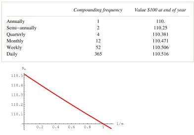
Table 4.1. Effect of compounding frequency on the value of $100 at the end of one year, when

Compounding frequency Value $100 at end of year

Annually 1 110.

Semi-_{annually 2 110.25}

Quarterly 4 110.381

Monthly 12 110.471

Weekly 52 110.506

Daily 365 110.516

0.2 0.4 0.6 0.8 1 1

êm 110.1

110.2 110.3 110.4 110.5 Rm

Figure 4.1: Effect of compounding frequency on the value of £100 after one year for an annualised interest rate of 10%.

Continuous Compounding

† _{In limit m}Ø ¶_{, obtain continuously compounded interest rates} † _{$100 grows to $100}‰R T _{when invested at a cc rate R for time T}

† _{$100 received at time T discounts to $100}‰-R T _{at time zero when the cc discount rate is R}

Conversion Formulas

Rc continuously compounded rate

Rm same rate with compounding m times per year

Equations relating discrete and continuous compounding rates

(4.1) Rc = mlnH1+ÅÅÅÅÅÅÅÅR_mmL

Rm = mH‰Rcêm-1L

RC =m lnI1+ÅÅÅÅÅÅÅÅÅÅR_mmM=2lnI1+ÅÅÅÅÅÅÅÅÅ0.1₂ M=0.09758

Example 4.2. Find the equivalent quarterly compounded interest rate corre-sponding to 8% with continuous compounding.

Rm=mI‰Rcêm-1M=4I‰0.08ê4-1M=0.0808

Zero Rates

Diagram of cashflows of zero-coupon and coupon-paying bonds

Code

Output

1 2 3 4 5 6 7 8 t

0.2 0.4 0.6 0.8 1 Cashflow

1 2 3 4 5 6 7 8 t

0.2 0.4 0.6 0.8 1 Cashflow

Figure 4.2: Cash flow diagrams for zero coupon (left) and coupon paying (right) bonds.

† _{n-year zero rate (zero-coupon rate, spot rate), starts today, lasts n-years}

† _{interest and principal (or face value or nominal value or par values) realized at the end of n} years — no intermediate payments

† _{interest earned on a zero coupon bond (zcb) or pure discount bond (pdb), whose value we} denote by BHt,TL

† _{Note that zcbs are a useful abstraction, but that most traded bonds are coupon bearing}

Zero rate

Definition 4.1. A zero rate (or spot rate), for maturity T is the rate of interest earned on an

investment that provides a payoff only at time T

Maturity (years) Zero Rate(% cont comp)

0.5 5.0

1.0 5.8

1.5 6.4

2.0 6.8

† _{Hull Table 4.2, page 81}

Sneak preview

† _{Why these ideas are so crucial to IR modelling} † _{Hull Chapters 28 & 29}

† _{Three alternative representations for the term structure}

PHt,TL price of zero-coupon bond maturing at time T, at any instant t§_T

YHt,TL yield to maturity of a zcb — is the slope of the chord to lnPHt,TL

fHt,TL instantaneous forward rate — is the slope of the tangent to lnPHt,TL

are related

(4.2)

PHt,TL= ‰-YHt,TLHT-tL_{= ‰}-_ŸtTfHt,sL„s

YHt,TL= ÅÅÅÅÅÅÅÅÅÅÅÅÅÅÅÅ-1

T-_t lnPHt,TL= 1 ÅÅÅÅÅÅÅÅÅÅÅÅÅÅÅÅ

T-_t ‡_t T

fHt,sL„_s

fHt,TL= -ÅÅÅÅÅÅÅÅÅÅÅÅÅÅÅÅÅÅÅÅÅÅ1

PHt,TL

∑_PH_t,TL ÅÅÅÅÅÅÅÅÅÅÅÅÅÅÅÅÅÅÅÅÅÅÅÅÅÅ

∑_T =YHt,TL+HT-tL

∑_YH_t,TL ÅÅÅÅÅÅÅÅÅÅÅÅÅÅÅÅÅÅÅÅÅÅÅÅÅÅ

∑_T

2 4 6 8 10T

0.3 0.4 0.5 0.6 0.7 0.8 0.9 δ

2 4 6 8 10T

-1.2 -1 -0.8 -0.6 -0.4 -0.2

Log@δD

2 4 6 8 10T

0.025 0.05 0.075 0.1 0.125 0.15 0.175 0.2

Y f

† _{To be continued in FM07...}

Bond pricing

Overview

† _{Price of coupon paying bond} † _{Bond yield}

† _{Par yield}

Price of coupon paying bond

† _{To calculate the cash price of a bond we discount each cash flow at the appropriate zero rate}

Example 4.3. Given the zero rates in the table above, price a 2-year Treasury bond, with principal $100 that pays a 6% per annum semi-annual coupon.

To calculate the PV of the

i k jjjjj jjjjj first second … y { zzzzz

zzzzz cashflow, we discount at

i k jjjjj jjjjj 5.0 5.8 … y { zzzzz zzzzz% for

i k jjjjj jjjjj 6 months 1 yr … y { zzzzz zzzzz.

$ 3õúúúúúúúúúúúúúúúúúúúúúúúúúúúúúúúú ‰-0.05ä0.5+úúúúúúúúúúúúúúúúù₃ ‰-0.058úúúúúúúúúúúúúúúúúúúúúúúúúúúúúúúúä1.0+₃ ‰-0.064úúúúúúúúúúúúúúä1.5û

Coupons prior to maturity

+ ₁₀₃

Coupon+principal

‰-0.068ä2.0=_$98.39

Mathematica demonstration

† _{We can program Mathematica to price a bond given} † _{yield curve in the form of a matrix of times and yields} † _{coupon, cm per annum}

† _{compounding frequency, m}

CouponBondHyieldCurve_? MatrixQ, cm_, m_L:=

ModuleA8T=_yieldCurveP₁T_,Y =_yieldCurveP₂T_,n=_Dimensions@_yieldCurveDP₂T<_,

100i k

jjjjj„-YPnTTPnT

JÄÄÄÄÄÄÄÄÄÄÄcm m

+1N+_‚

i=1

n-1 cm ÄÄÄÄÄÄÄÄÄÄÄ

m

„-YPiTTPiTy

{ zzzzzE † _{E.g. let us check the example above}

WithA9yieldCurve=J0.5` 1 1.5` 2.`

0.05` 0.058` 0.064` 0.068`N, cm=0.06, m=2=, CouponBond@yieldCurve, cm, mDE

98.3851

Bond yield

Definition 4.2. The bond yield for a bond is the discount rate that makes the present value of

the cash flows equal to the market price.

† _{Also yield to maturity or bond equivalent yield} Equation for bond yield

† _{The bond yield (continuously compounded) is given by solving}

(4.3) ‚

i=1 n

c‰-YTi õúúúúúúúúúúúúùcouponsúúúúúúúúúúû

+ ₁õúúúúúúúúù û ‰-YúúúúúúTn

principal

=_P

where

n number of cashflows c coupon paymentcashflow

Ti time of ith payment (coupon or principal) payment, i=_1,…,n P given (market) price of bond

Y bond yield

† _Note, ⁄i₌ 1

n _c‰-Y Ti+ ‰-Y Tn= ⁄i =1

n-1_c‰-Y Ti+H₁+_cL‰-Y Tn

Example

Example 4.4. Find the bond yield for a 2-year Treasury bond, with principal $100 with market price equal to $98.39.

Numerical root search. Could use Solver in Excel. Here we will use Mathematica ’s FindRoot function....

Mathematica experiment

† _{We can program Mathematica to price a bond given} † _{times for coupon payments (vector)}

† _{yield (scalar, to apply to all maturities, corresponding to a flat yield curve)} † _{coupon, cm, annualised}

† _{compounding frequency, m}

CouponBondFlatYieldHT_List, Y_, cm_, m_L:=

ModuleA8n=_Length@TD<_{, 100} i

k jjjjj jjj„-Y TPnT

JÄÄÄÄÄÄÄÄÄÄÄcm m

+₁N+_„

i=1

n-1

cm„-Y TPiT

ÄÄÄÄÄÄÄÄÄÄÄÄÄÄÄÄÄÄÄÄÄÄÄÄÄÄÄÄÄÄÄÄÄÄÄÄ m

y

{ zzzzz zzzE

CouponBondFlatYield@80.5`, 1, 1.5`, 2.`<, Y, 0.06, 2D

100H1.03−2. Y_+0.03−1.5 Y_+0.03−Y_+0.03−0.5 Y_L

† _{Plot this}

Plot@CouponBondFlatYield@80.5`, 1, 1.5`, 2.`<, Y, 0.06, 2D,

8Y, 0, 0.4<, PlotStyle−>8Thickness@0.01D, Hue@0D<, AxesLabel−>8"Y", "PHYL"<, PlotRange−>80, 120<D;

0.1 0.2 0.3 0.4Y

20 40 60 80 100 120

PHYL

† _{Numerically solve for the bond yield, Y, such that our calculated bond price agrees with the} market price

FindRoot@CouponBondFlatYield@80.5`, 1, 1.5`, 2.`<, Y, 0.06, 2D==98.39,

8Y, 0.1<D 8Y→0.0675982<

† _{Check: when we take the bond yield to be 6.76%, is the calculated bond price $98.39 as we} require?

CouponBondFlatYield@80.5`, 1, 1.5`, 2.`<,0.067598, 0.06, 2D

98.39

Answer

...

Bond yield is y=_{0.0676 or 6.76%.}

Discrete case

† _{Hull develops ideas for price of zcb using continuous compounding "B}H_0,TL= ‰-YCH0,TLT_". † _{Analogous expressions exist for discrete case "B}H_0,iL=_{ÅÅÅÅÅÅÅÅÅÅÅÅÅÅÅÅ}1_{ÅÅÅÅÅÅÅÅÅÅÅ}

Par yield

Definition 4.3. The par yield for a certain maturity is the coupon rate that causes the bond

price to equal its face value.

Equation

(4.4) 100i

k jjjjj‚

i=1 n-1

c‰-YiTi₊H_1+cL_‰-YiTiy

{ zzzzz=₁₀₀

where

n number of cashflows, Hn-₁L _{of which are coupons, and the nth is} coupon + principal

c coupon payment

Ti time of ith payment (coupon or principal) payment, i=1,…,n Yi bond yield Hzero rateLfor timeTiTypo

† _{Solving for c}

(4.5) c= 1- ‰

-YnTn ÅÅÅÅÅÅÅÅÅÅÅÅÅÅÅÅÅÅÅÅÅÅÅÅÅÅÅÅÅÅÅÅÅ

⁄i=1 n _‰-YiTi

† _{Here c is the actual coupon payment}

† _{Often coupon rates are quoted assuming a frequency m, in which case the annualised} coupon rate cm satisfies c=cmêm.

† _{If we name d}= ‰-YnTn _{and A}=⁄i =1

n _‰-YiTi_{, we obtain}

(4.6) cm=ÅÅÅÅÅÅÅÅÅÅÅÅÅÅÅÅH1-dÅÅÅÅÅÅÅÅÅÅÅÅLm

A

Example 4.5. Find the annualised par yield for a 2-year Treasury bond, making semi-annual coupon payments, with principal $100 with market price equal to $98.39.

c2 ÅÅÅÅÅÅÅÅ

2 ‰

-0.05ä0.5_{+ÅÅÅÅÅÅÅÅ}c2

2 ‰

-0.058ä1.0_{+ÅÅÅÅÅÅÅÅ}c2

2 ‰

-0.064ä1.5_{+I1+ÅÅÅÅÅÅÅÅ}c2

2 M ‰

-0.068ä2.0₌₁

c2= 2I1

-‰-0.068ä2.0_M

ÅÅÅÅÅÅÅÅÅÅÅÅÅÅÅÅÅÅÅÅÅÅÅÅÅÅÅÅÅÅÅÅÅÅÅÅÅÅÅÅÅÅÅÅÅÅÅÅÅÅÅÅÅÅÅÅÅÅÅÅÅÅÅÅÅÅÅÅÅÅÅÅÅÅÅÅÅÅÅÅÅÅÅÅÅÅÅÅÅÅÅÅÅÅÅÅÅÅÅÅÅÅÅÅÅÅÅÅÅÅÅÅÅÅÅÅÅÅÅÅÅ

‰-0.05ä0.5+‰-0.058ä1.0+‰-0.064ä1.5+‰-0.068ä2.0 =6.87% (annualized)

or taking A= ‰-0.05ä0.5_{+ ‰}-0.058ä1.0_{+ ‰}-0.064ä1.5_{+ ‰}-0.068ä2.0_{=3.70027 and d= ‰}-0.068ä2.0_=0.87284

† _{Check algebra}

WithA8A= −0.05 0.5₊ −0.058 1.0₊ −0.064 1.5₊ −0.068 2.0_{, d=} −0.068 2.0<_,

9A, d, 2 H1−dL

A =E

83.70027, 0.872843, 0.0687288<

Mathematica experiment

† _{Use the function for the coupon paying bond in terms of the yield curve}

WithA9yieldCurve=J0.5` 1 1.5` 2.`

0.05` 0.058` 0.064` 0.068`N, m=2=,

Solve@CouponBond@yieldCurve, cm, mD==100, cmDE

88cm→0.0687288<<

Determining zero rates

† _{How to calculate Treasury zero rates from the prices of Treasury bonds}

Sample data

† _{Hull Table 4.3, page 82}

† _{Data for 5 bonds, 2 paying coupons semi-annually} † _Principal

† _{Time to maturity} † _Coupon

† _{Market price}

Make table

Code

Output

Table 4.3. Data for 5 bonds, 2 paying a semi-annual coupon

Principal Time to maturity Coupon Cash price

100 0.25 0 97.5

100 0.5 0 94.9

100 1. 0 90.

100 1.5 8. 96.

100 2. 12. 101.6

The bootstrap method

• An amount 2.5 can be earned on 97.5 during 3 months. The annualised 3-month rate is 4100-_97.5

ÅÅÅÅÅÅÅÅÅÅÅÅÅÅÅÅÅÅÅÅÅÅÅÅÅ

97.5 =4

2.5

ÅÅÅÅÅÅÅÅÅÅÅÅÅ

97.5 =0.10256 or 10.256% with quarterly compounding. This is 10.127% with

continu-ous compounding

Rc = m lnI1+ÅÅÅÅÅÅÅÅÅÅR_mmM =4 LogA1+ÅÅÅÅÅÅÅÅÅÅÅÅÅÅÅÅÅÅÅÅÅÅ0.10256₄ E=0.101267

• Similarly the 6 month and 1 year rates are 10.469% and 10.536% with continuous compounding 2 LogA1+_{ÅÅÅÅÅÅÅÅÅÅÅÅÅÅÅÅ}2H100-_{ÅÅÅÅÅÅÅÅÅÅÅÅÅÅÅÅ}94.9Lê_{ÅÅÅÅÅÅÅÅÅÅÅÅÅ}94.9

2 E=0.104693

1 LogA1+_{ÅÅÅÅÅÅÅÅÅÅÅÅÅÅÅÅ}1H100-_{ÅÅÅÅÅÅÅÅÅÅÅÅÅÅÅÅÅÅÅ}90Lê90

1 E=0.105361

• To calculate the 1.5 year rate we solve 4 ‰-0.10469ä0.5_{+4 ‰}-0.10536ä1.0_{+104 ‰}-Rä1.5₌₉₆

R= -ÅÅÅÅÅÅÅÅÅ1

1.5LogA

96-_I4 ‰-0.10469ä0.5+4 ‰-0.10536ä1.0_M ÅÅÅÅÅÅÅÅÅÅÅÅÅÅÅÅÅÅÅÅÅÅÅÅÅÅÅÅÅÅÅÅÅÅÅÅÅÅÅÅÅÅÅÅÅÅÅÅÅÅÅÅÅÅÅÅÅÅÅÅÅÅÅÅÅÅÅÅÅÅÅÅÅÅÅÅÅÅÅÅÅÅÅÅÅÅÅÅÅÅÅÅÅ

104 E

to get R =_{0.10681 or 10.681%}

• Similarly the two-year rate is 10.808% 6 ‰-_0.10469ä_0.5+

6 ‰-_0.10536ä_1.0+

6 ‰-_0.10681ä_1.5+

106 ‰-Rä_2.0= 101.6 R= -ÅÅÅÅÅÅÅÅÅ1

2.0 LogA

101.6-_I6 ‰-0.10469ä0.5+₆ ‰-0.10536ä1.0+₆ ‰-0.10681ä1.5_M ÅÅÅÅÅÅÅÅÅÅÅÅÅÅÅÅÅÅÅÅÅÅÅÅÅÅÅÅÅÅÅÅÅÅÅÅÅÅÅÅÅÅÅÅÅÅÅÅÅÅÅÅÅÅÅÅÅÅÅÅÅÅÅÅÅÅÅÅÅÅÅÅÅÅÅÅÅÅÅÅÅÅÅÅÅÅÅÅÅÅÅÅÅÅÅÅÅÅÅÅÅÅÅÅÅÅÅÅÅÅÅÅÅÅÅÅÅÅÅÅÅÅÅÅÅÅÅÅÅÅÅÅÅÅÅÅÅÅÅ

106 E

Some checks

Figure of zero curve

Code

Output

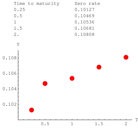
Table 4.4. Yield curve obtained by bootstrapping

Time to maturity Zero rate

0.25 0.10127

0.5 0.10469

1 0.10536

1.5 0.10681

2. 0.10808

0.5 1 1.5 2 T

0.102 0.104 0.106 0.108 Y

Figure 4.4: Yield curve obtained by bootstrapping

Interpolation

† _{Simple approach: linear (straight lines between points)} † _{Splines etc.}

Forward rates

Definition

Definition 4.4. The forward rate is the future zero rate implied by today’s term structure of

interest rates † _{Basic idea:}

† _{given time 0 cost of $1 at time T1} † _{given time 0 cost of $1 at time T2}

† _{at time 0 lock in the time T1 cost of $1 at T2:} "BH0,T2L=BH0,T1LBH0,T1,T2L"

† _{Each bond (spot or forward) has a rate associated with it (spot or forward)} "‰-T2YH0,T2L= ‰-T1YH0,T1L ‰-HT2-T1LYH0,T1,T2L_"

Calculation of forward rates

Example 4.7. The continuously compounded zero rates for n-year investment are given by the following matrix (upper row is n, lower row is zero rate):

i k

jjj1_{3.0 4.0 4.6 5.0 5.3}2 3 4 5 y_{zzz.

• What does it mean to say that the 1-year rate is 3.0% and the 2-year rate is 4.%?

• What rate of interest (the “forward” interest) holds over year 2 such that if combined with the rate of interest over year 1 equals the overall rate of interest over the two years?

• Find the forward rates for borrowing over the nth year for n=2, …5. • The 1-year continuously compounded rate is 3.0% means that £100 invested now will grow to £100‰0.03=_{£103.05 over 1 yr}

• The 2-year continuously compounded rate is 4.0% means that £100 invested now will grow to £100‰0.04ä₂₌

£108.33 over 2 yrs

• 100 ‰-_0.03ä₁

spot

‰forward-R_Fä₁₌

100 ‰-_0.04ä₂

spot

RF =ÅÅÅÅÅÅÅÅÅÅÅÅÅÅÅÅ0.04ä2ÅÅÅÅÅÅÅÅÅÅÅÅÅÅÅÅÅÅÅÅÅÅ-₁0.03ä1 =0.05

H L

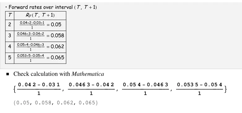
T RFHT , T+1L

2 ÅÅÅÅÅÅÅÅÅÅÅÅÅÅÅÅ0.04ä2ÅÅÅÅÅÅÅÅÅÅÅÅÅÅÅÅÅÅÅÅÅÅ-0.03ä1

1 =0.05

3 0.046ä₃-_0.04ä₂ ÅÅÅÅÅÅÅÅÅÅÅÅÅÅÅÅÅÅÅÅÅÅÅÅÅÅÅÅÅÅÅÅÅÅÅÅÅÅÅÅÅÅ

1 =0.058

4 _{ÅÅÅÅÅÅÅÅÅÅÅÅÅÅÅÅ}0.05ä4_{ÅÅÅÅÅÅÅÅÅÅÅÅÅÅÅÅ}-0.046_{ÅÅÅÅÅÅÅÅÅÅ}ä3 1 =0.062

5 ÅÅÅÅÅÅÅÅÅÅÅÅÅÅÅÅ0.053äÅÅÅÅÅÅÅÅÅÅÅÅÅÅÅÅ5-0.05ÅÅÅÅÅÅÅÅÅÅä4

1 =0.065

† _{Check calculation with Mathematica}

90.04 2−0.03 1

1 ,

0.046 3−0.04 2

1 ,

0.05 4−0.046 3

1 ,

0.053 5−0.05 4

1 =

80.05, 0.058, 0.062, 0.065<

Check

Code

Output

table: fwd rates

Table 4.5. Zero rates for n-year investment and forward rates for borrowing for one year

inferred from these.

T Zero rate Fwd rate

1 3. 0

2 4. 5.

3 4.6 5.8

4 5. 6.2

5 5.3 6.5

Formula for forward rates

† _{Suppose that the zero rates for time periods T1 and T2 are R1 and R2 with both rates} continu-ously compounded.

† _{The forward rate for the period between times T1 and T2 is}

(4.7) RF =

R2T2-R1T1 ÅÅÅÅÅÅÅÅÅÅÅÅÅÅÅÅÅÅÅÅÅÅÅÅÅÅÅÅÅÅÅÅÅÅÅÅÅÅÅÅÅ

T2-T1

Derivation † _{Not in Hull}

† _{Result is more intuitive using a different notation:}

Ti maturity times of bonds, i=1,2, 0<T1<T2 BH0,TiL cost at time 0 for a zcb maturing at time Ti, i=1,2

BH0,T1,T2L time 0 forward price for a bond at time T1 maturing at time T2 YH0,TiL spot yield over interval H0,TiL — i.e. Ri

† _{Relationship between spot and forward bond prices}

BH0,T2L=BH0,T1LBH0,T1,T2L † _{Implies relationship between spot and forward yields}

‰-T2YH0,T2L_{= ‰}-T1YH0,T1L _‰-HT2-T1LYH0,T1,T2L † _{Solve for Y}H_0,T1,T2L

Instantaneous forward rate

Definition 4.5. The instantaneous forward rate for a maturity T is the forward rate that

applies for a very short time period starting at T. It is RF =R+T ∑R ÅÅÅÅÅÅÅÅ ∑T where R is the T-year rate

(4.8) RF=R+T

∑_R

ÅÅÅÅÅÅÅÅÅÅÅ

∑_T

Upward vs downward sloping yield curve

† _upward

Fwd Rate>_{Zero Rate}>_{Par Yield}

† _downward

Par Yield > _{Zero Rate} > _{Fwd Rate}

Forward rate agreement

† _{Might be used by company that wishes to borrow cash at a future date T1 for the period} @T1,T2D

† _{Locks in rate of interest} † _{Cash flow determined by}

† _{length of time-period} † _{interest rates:}

† _prespecified

† _{prevailing at the future time}

† _{Forward contract on uncertain future cash flow}

† _{Can synthesise with forward-forward loan – LT loan + ST deposit}

Definition

Definition 4.6. A forward rate agreement (FRA) is an agreement that a certain rate will

apply to a certain principal during a certain future time period. † _{Interest payments exchanged – predetermined RK} ¨ _{market RF}

FRA valued by assuming that the forward interest rate is certain to be realized

Payoffs

† _{Hull Equations 4.9 and 4.10 page 88} † _Notation

RK IR agreed to in FRA

RF forward LIBOR IR for period @T1,T2D calculated today

RM actual LIBOR IR observed in the market at T1 for interval @T1,T2D L principal

† _{Compounding frequency reflects maturity} † _{X lends to Y}

† _{Normally at LIBOR RM} † _FRA fl _{X earns RK instead} † _{Extra interest due to FRA}

(4.9) LHRK-_RMLH_T2-_T1L

† _{Y gets minus this}

† _{X receives fixed, pays market; Y pays fixed, receives market,} † _{FRAs settled at T2}

Settlement in advance † _{Usually, settled at time T1}

† _{Payment at T2, discounted back to T1} † _{Company X’s payoff at T1:}

(4.10) LHRK-_RMLH_T1-_T2L

ÅÅÅÅÅÅÅÅÅÅÅÅÅÅÅÅÅÅÅÅÅÅÅÅÅÅÅÅÅÅÅÅÅÅÅÅÅÅÅÅÅÅÅÅÅÅÅÅÅÅÅÅÅÅÅÅÅÅÅÅÅÅÅÅ 1+_RMH_T2-_T1L

Example

Example 4.8. A company enters into an FRA so that it will receive 4% fixed on a principal of $1 million for a 3-month period starting in 3 years. If LIBOR turns out to be 4.5%, find the cashflow to the lender at the end of the borrowing period and the equivalent cashflow at the start of the borrowing period, expressing all interest rates using quarterly compounding.

Cashflows

At end of period: T2

$106_{äH0.04-0.045Lä0.25= -$1250}

At start of period: T1

-_$ÅÅÅÅÅÅÅÅÅÅÅÅÅÅÅÅ1250ÅÅÅÅÅÅÅÅÅÅÅÅÅÅÅÅÅÅÅÅ

1+_0.045ä_0.25 =$1236.09

Valuation

† _{Key observation:}

FRA worth zero when RK=RF

† _{Why buy an FRA for $$ if you can lock in price of forward borrowing} † _{E.g. borrow} @_0,T1D_{, lend} @_0,T2D_{; borrowing costs} @_T1,T2D _{locked at time 0.} † _{Go long FRA with rate RK, short FRA with rate RF}

† _{Costs are VFRA and 0 respectively}

† _{Net (deterministic) payoff at T2 is L}HH_RK-_RML-H_RF-_RMLLH_T1-_T2L

† _{Value of FRA where a fixed rate RK will be received on a principal L between times T1 and} T2 is

(4.11) VFRA=õúúúúúúúúúúúúúúúúúúúúúúúùLHRK-RFLúúúúúúúúúúúúúúúúúúúúúHT1-T2Lû

Cash flow at timeT2

‰-R2T2

† _{Value of FRA where a fixed rate is paid is minus this}

† _{RF is the forward rate for the period and R2 is the zero rate for maturity T2} Example

Rm = mI‰Rcêm-1M =1

i

k jjjjj jj‰0.05

Fwd

ì1

-₁y

{ zzzzz

zz=0.05127=RF

VFRA=LHRK -RFLHT2-T1L ‰-R2T2=$106äH0.06-0.05127L‰- 0.04

2 yr spot ä₂₌

$8058

Duration

† _{Hull page 89}

† _Name fl _{average time to receive payments}

Definition

Definition 4.7. The duration of a bond that provides cash flow ci at time ti is

D=‚ i=1 n

ti_{ÅÅÅÅÅÅÅÅÅÅÅÅÅÅÅÅÅ}ci ‰-y ti

B

where B is its price and y is its yield (continuously compounded)

† _{Cf. “centre of mass”}

Sensitivity

(4.12)

D_B

ÅÅÅÅÅÅÅÅÅÅÅ

B = -DDy

Example

Example 4.10. Express the price of a bond, B, in terms of a sum of n dis-counted cash flows, ci, paid at time ti, t=1, …,n, assuming a constant, continu-ously compounded yield y. Differentiate this w.r.t. y to obtain an expression for the duration D= -_ÅÅÅÅÅ1

B

„B

ÅÅÅÅÅÅÅÅ

„y. In what sense is this the average maturity of the instrument?

B=_⁄i=

1

n _c

i ‰-y ti

„_B ÅÅÅÅÅÅÅÅÅ

„_y = -⁄i=1

n _t

ici ‰-y ti

D= -ÅÅÅÅÅÅ1

B

„B

ÅÅÅÅÅÅÅÅÅ

„y =„_i=1 n

ti ci

‰-y ti ÅÅÅÅÅÅÅÅÅÅÅÅÅÅÅÅÅÅÅÅÅÅÅ

Interpretation

Duration is the proportional change in the bond price per unit (parallel) shift in the yield curve

Example

Example 4.11. Calculate the duration of a 3-year bond paying semi-annuallly a coupon of 10% (annualized), with a face value of $100 and a yield of 12% (continuously compounded).

Time Cash flow PV Wt Wtä_time 0.5 5 5ä ‰-0.12ä0.5=_4.709 ÅÅÅÅÅÅÅÅÅÅÅÅÅÅÅÅÅÅ4.709

94.213 =0.050 0.025

1.0 5 5ä ‰-_0.12ä_1.0=

4.435 ÅÅÅÅÅÅÅÅÅÅÅÅÅÅÅÅÅÅ4.435

94.213 =0.047 0.047

1.5 5 5ä ‰-0.12ä1.5_{=4.176 ÅÅÅÅÅÅÅÅÅÅÅÅÅÅÅÅÅÅ}4.176

94.213 =0.044 0.066

2.0 5 5ä ‰-0.12ä2.0=_3.933 ÅÅÅÅÅÅÅÅÅÅÅÅÅÅÅÅÅÅ3.933

94.213 =0.042 0.083

2.5 5 5ä ‰-_0.12ä_2.5=

3.704 ÅÅÅÅÅÅÅÅÅÅÅÅÅÅÅÅÅÅ3.704

94.213 =0.039 0.098

3.0 105 105ä ‰-0.12ä3.0_{=73.256 ÅÅÅÅÅÅÅÅÅÅÅÅÅÅÅÅÅÅÅ}73.256

94.213 =0.778 2.333

Total 130 B=_{94.213 1.000 D}=_2.653

Example

Example 4.12. Using the bond from the previous example, find the change in the bond price for a 10 basis point increase in the yield

i) approximately using your knowledge of the duration ii) exactly

i) B+ DB=B-B DDy=_94.213-_94.213ä_2.653ä_0.001= 94.213 bond price 12% yield

-_0.250

change

= _93.963

bond price 12.1% yield

ii) ⁄in=₁ci ‰-y ti»y=_0.121=5ä ‰-0.121ä0.5+…+105ä ‰-0.121ä3.0 =93.963 Same to 3dp!

Modified duration

† _{So far, continuous compounding}

† _{When the yield y is expressed with compounding m times per year}

(4.13) D_B= -ÅÅÅÅÅÅÅÅÅÅÅÅÅÅÅÅBDDÅÅÅÅÅÅÅy

1+ÅÅÅÅÅy m

Definition 4.8. The modified duration is given by the expression

Dè = _{ÅÅÅÅÅÅÅÅÅÅÅÅÅ}D 1+_ÅÅÅÅÅy

Example

Example 4.13. For the bond in the previous examples, find the yield for semi-annual compounding, the modified duration, the approximate decrease in the bond price if the yield increases by 10 basis points, and the new bond price.

Rm=mI‰Rcêm-1M=2I‰0.12ê2-1M=0.123673

Dè=ÅÅÅÅÅÅÅÅÅÅÅÅÅÅD

1+ÅÅÅÅÅÅÅÅy m

=ÅÅÅÅÅÅÅÅÅÅÅÅÅÅÅÅ2.653ÅÅÅÅÅÅÅÅÅÅÅÅÅÅÅ

1+ÅÅÅÅÅÅÅÅÅÅÅÅÅÅÅÅ0.123673ÅÅÅÅÅÅÅÅÅÅÅÅÅÅÅÅÅÅ 2

=_2.4985

D_B= -_{B D}èD_y= -_94.213ä_2.4985ä_0.001= -_0.234 B '=_94.213-_0.235=_93.978

Convexity

† _{The convexity of a bond is defined as}

(4.14) C= ÅÅÅÅÅÅ1

B

∑2_B

ÅÅÅÅÅÅÅÅÅÅÅÅÅÅ

∑_y2 =‚i=1

n

t_i2 ci ‰ -y ti ÅÅÅÅÅÅÅÅÅÅÅÅÅÅÅÅÅÅÅÅÅÅ

B

so that

(4.15)

D_B

ÅÅÅÅÅÅÅÅÅÅÅ

B = -DDy+ 1 ÅÅÅÅÅ

2 CHDyL 2

Theories of the term structure

† _{Expectations Theory: forward rates equal expected future zero rates [long IRs] = [short} IRs]

† _{No reason to believe a downward sloping yield curve implies falling rates.} † _{Is true under RNM , in arb-free market}

† _{Market Segmentation: short, medium and long rates determined independently of each other} † _{Supply and demand for short / medium / long term debt}

† _{Liquidity Preference Theory: forward rates higher than expected future zero rates} † _ET fl _{long IRs = short IRs; however:}

† _{investors – preserve liquidity so prefer short end} † _{borrowers – fixed rates for long periods}

† _{to clear market, short} ∞_{, long}  † fl _{forward rates > future zero-rates} † _{usually observed}

† _{Hull Page 93, Musiela and Rutkowski P332}

Summary

† _{Important rates for derivatives} † _Treasury

† _LIBOR

† _{Rate depends on compounding rates; as frequency} ض_{, continuous compounding} † _Rates

† _{n-year zero – investment lasts n years, all return realized at end}

† _{bond yield – for bond with particular maturity, is flat yield s.t. theoretical and market} prices match

† _{par yield – for bond with particular maturity, is coupon s.t. theoretical and par prices} match

† _{forward – rates for intervals of time in future implied by current zero rates} † _{Bootstrapping zero curve from prices of coupon bonds}

† _{Forward rate agreement (FRA)}

† _{OTC agreement; certain IR for principal in return for LIBOR over future interval} † _{Value – assume fwd rates realized and discount payoff}

† _{Duration – sensitivity of value of bond (portfolio) to parallel shift in yield curve} † _{Convexity – 2nd order sensitivity of value of bond (portfolio) to parallel shift in yield}

curve; “curvature"

D_B

ÅÅÅÅÅÅÅÅÅÅÅ

B = -DDy+ 1 ÅÅÅÅÅ 2 CHDyL

2