Tools for sampling Multivariate Archimedean Copulas

(1)

Tools for sampling Multivariate Archimedean Copulas

Mario R. Melchiori CPA†

Universidad Nacional del Litoral Santa Fe - Argentina

March 2006

Abstract

A hurdle for practical implementation of any multivariate Archimedean copula was the absence of an efficient method for generating them. The most frequently used approach named conditional distribution one, involves differentiation step for each dimension of the problem. For this reason, it is not feasible in higher dimension. Marshall and Olkin proposed an alternative method, which is computationally more straightforward than the conditional distribution approach. We present the tools necessary for understand it and use it. We introduce the Laplace Transform and its role in the generation of multivariate Archimedean copulas. In order to cover the gap between the theory and its practical implementation VBA code and R one are provided.‡

The prices do not follow models. We invent models to describe prices. Glyn Holton – www.contingencyanalysis.com

(2)

Introduction

A hurdle for practical implementation of any multivariate Archimedean copula was the absence of an efficient method for generating them. The most frequently used approach named conditional distribution one, involves differentiation step for each dimension of the problem. For this reason, it is not feasible in higher dimension. Marshall and Olkin proposed an alternative method, which is computationally more straightforward than the conditional distribution approach. A disadvantage is that it requires the generation of an additional variable. For bivariate applications, this means generating 50% more uniform random variables, but for higher dimension that drawback is negligible.

We describe now the algorithm to generate multivariate Archimedean copula. The d-dimensional Archimedean copulas may be written as:

( ) 1( ( ) ( ))

1

,...,

d 1

...

d

,

C u

u

=

φ

−

φ

u

+

u

Where

φ

is a decreasing function known as the generator of the copula and

φ

−1denotes the inverse of the generator

(Frees and Valdez; McNeil et al.). In addition,

φ

−1is equal to the inverse of the Laplace transformLaplace transformLaplace transform of a distribution Laplace transform

function

G

on

+satisfying

G

( )

0 =

0

, the following algorithm can be used for simulating from the copula:

Algorithm 1:

1. Simulate

d

independent uniform variable

u

i

for i

=

1,...,

d

2. Simulate a variable

Y

with distribution function

G

such that the Laplace transformLaplace transformLaplace transform of Laplace transform

G

is the inverse of the generator.

3. Define i

ln

( i)

1,...,

u

s

for i

d

Y

−

=

4. Define

X

i

=

φ

−1( )

s

i

for i

=

1,...,

d

Then

X

₁

,...

X

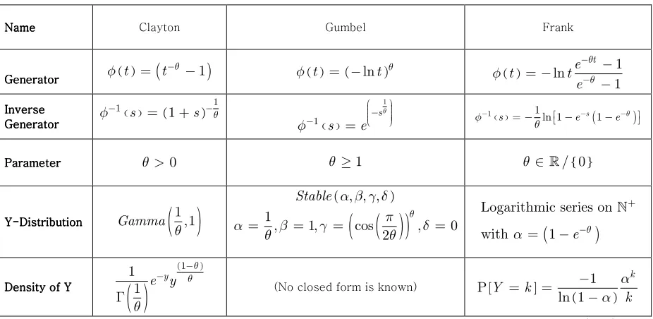
d have Archimedean copula dependence structure.

[image:2.612.91.554.439.665.2]

Table Table Table

Table IIII:::: Some generators for Archimedean copulas, their inverses and their Laplace transforms. Source: Marshall and Olkin (1988).

Though the density of a

α

−

stable

distribution’s closed form is not known Nolan proposed the following simulation algorithm for generating random variables

α

−

stable

distributed:

Name Name Name

Name Clayton Gumbel Frank

Generator Generator Generator

Generator ( )

t

(

t

1 )

θ

φ

=

−

_φ

( )

t

_{= −}

(

ln

t

)θ _{( )}

_ln

1

t

e

t

e

θ θ

φ

− −

−

= −

−

Inverse Inverse Inverse Inverse Generator Generator Generator Generator ( ) ( ) 1

1

_s

₁

_s

θ

φ

−

=

+

−

( )

1

_s

_e

s θ

φ

 _  _ −   _ 

−

₌

  _φ 1(_s) 1_{ln 1} _e s

(

₁ _e θ

)

θ − _{= −} _ ₋ − ₋ − _   Parameter Parameter Parameter

Parameter

θ

>

0 θ

≥

1 θ

∈

/ 0

{ }

Y Y Y

Y---Distribution-DistributionDistributionDistribution

Gamma

( )

1 ,1

θ

(

, , ,

)

Stable

α β γ δ

( )

(

)

1 ,

1,

cos

,

0

2

θ

π

α

β

γ

δ

θ

=

₍

₎

+

Logarithmic series on

with

α

=

1 −

e

−θ

Density of Y Density of Y Density of Y Density of Y

( )

(1 )

1

1 e

y

θ θ

θ

− −

Γ

(No closed form is known) [ ] ( )

1 ln 1

k

Y

k

α

−

Ρ

=

(3)

Algorithm 2:

1. Simulate an uniform variable

(

,

)

2 2

U

π π

Θ

∼

−

2. Simulate an exponentially distributed variable

W

with mean 1 independently of

Θ

. 3. Set

θ

₀

=

arctan

(

β

tan

(

πα

/ 2 /

)

α

.

4. Compute

Z

∼

St

(

α β

, ,1, 0

)

(

)

(

)

(

)

( )

(

)

(

)

1 sin

₀

cos

₀

1 ₁

1/

cos

₀

cos

2

2 ₂

tan

ln

=1

2 Z

W

Z

α

α θ

αθ

α

_α

α

αθ

π

β

_π

α

π

_β

−





+ Θ

_

+

−

Θ

_

_≠

=

_

_





Θ





_

_{Θ }







_



_







=

_

+ Θ

Θ −

_



_

_



+ Θ



















5. Compute

X

∼

St

(

α β γ δ

, , ,

):

( )

(

2

)

1 ln

1 X

Z

X

Z

γ

δ

α

γ

δ

β

γ

α

π

=

+

≠

=

+

=

Below, we use Kemp’s second accelerated generator of Logarithmic Distribution random variables from Luc Devroye’s book titled “Non-Uniform Random Variate Generation” chapter 10, page 548, freely available on

http://cgm.cs.mcgill.ca/~luc/rnbookindex.html.

Algorithm 3

Algorithm 3::::

Set

c

=

ln 1

(

−

α

)

Simulate an uniform variable

V

[

0,1

]. IF

IFIF

IF

V

≥

α

then set

X

=

1

ELSE ELSEELSE ELSE

Simulate an uniform variable

U

[

0,1

].

Set

_q

_{= −}

1 _e

cU

CASE CASECASE CASE

2

_:

V

≤

q

set ( )

( )

ln

int 1

ln

V

X

q





=



_

+



_





. 2

_:

q

<

V

≤

q

set

X

=

1

.

:

V

>

q

set

X

=

2

.

X

is Logarithmic Series distributed.

No other algorithm is necessary because the most of software have a built-in function that generates random variables Gamma distributed, such as GammaInv GammaInv GammaInv GammaInv function on Excel and rgammargammargamma on R. rgamma

Laplace Transform

The Laplace TransformLaplace TransformLaplace Transform of a function Laplace Transform

f t

( ) is denoted by

L

[

f t

( )]and defined by:

L

[ ( )] ( )

0

st

f t

f t e

dt

∞

−

=

_∫

(4)

[image:4.612.190.443.119.360.2]

L

−1[

_{f s}

( )]

=

_{f t}

( ).

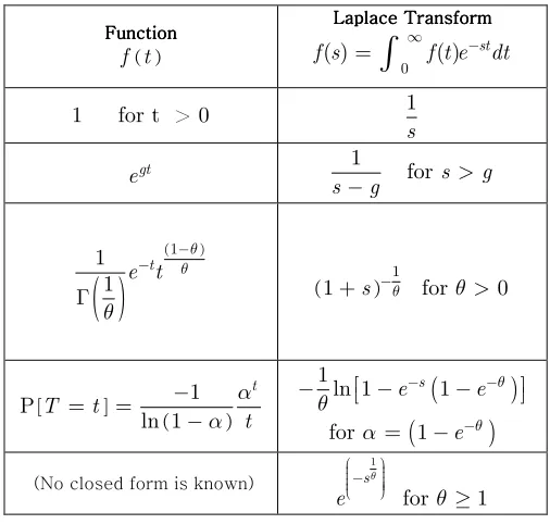
Table of Laplace TransformLaplace TransformLaplace TransformLaplace Transform pairs, which are of interest for our work:

Function FunctionFunction Function ( )

f t

Laplace Transform Laplace Transform Laplace Transform Laplace Transform 0

( )

st

f s

=

∫

∞

f t e

−

dt

1 for t > 0

1 s

gt

e

_s

₋

1 _g

for

s

>

g

( )

(1 )

1

t

e t

θ θ

θ

− −

Γ

( )

1

1 +

s

−θ

for

θ

>

0

[ ] ( )

1 ln 1

t

T

t

α

−

Ρ

=

−

(

)

1 ln 1

_e

s

1 _e

θ

− −





−

_

−

_

(

)

for

α

=

1 −

e

−θ

(No closed form is known)

1

for

1

s

e

θ

 _  _ −   _  

_≥

Table Table Table

Table IIIIII -II--- Laplace Transform pairs

From an economic point of view we immediately recognize the Laplace transformLaplace transformLaplace transformLaplace transform as the present value of a stream of returns

f t

( )at the interest rate

s

. The present value of cash flows of $1,

f t

( )

=

1

, paid annually and perpetually at the continuous interest rate

s

is

L

[ ( )]

0

1

st

f s

e

dt

s

∞

−

=

_∫

=

. On the other hand, the present discounted value at the

continuous interest rate

s

of a cash flow growing at the rate

g

,

_{f t}

( )

₌

_e

gt_{, is}

_L

_[ ₍ ₎_] 0

1

gt st

f s

e e

dt

s

g

∞ −

=

−

∫

. If

( )

f t

is continuous and differentiable at all

t

≥

₀

, then it is possible to recover

f t

( ) from

L

[

_{f s}

( )]through the inverse transformation:

L

1[ ( )] ( )

_lim

1

2

a ib st b

a ib

f s

f t

e

i

π

+ −

→∞ ₋

=

_∫

L

[

_{f s ds a}

( )]

_,

≥

_α

.

This has the economic meaning that if we know the present discounted value of a stream of returns at every interest rate, we can recover the whole pattern of the stream of returns.

Experiment I

We conduct an experiment for seeing practically in what manner, by knowing the Laplace transform of a function, we can recover it. We will do it here, but you can reproduce it on your own computer. For doing this, we need an approach that implements numerically the inverse transformation

L

−1[

_{f s}

( )]. We will use the Euler1_{method. Readers interested}

in deepeningthis subject should consult the following link:

http://www.columbia.edu/~ww2040/Laplace http://www.columbia.edu/~ww2040/Laplacehttp://www.columbia.edu/~ww2040/Laplace

http://www.columbia.edu/~ww2040/LaplaceInversionJoC95.pdfInversionJoC95.pdfInversionJoC95.pdfInversionJoC95.pdf

(5)

The experiment consists of computing the flow of returns by knowing its net present value using the inverse Laplace

transform

.

As we already saw, the net present value of a stream of returns that grows to the continuous rate

g

,

represented by the function

_{f t}

( )

₌

_e

gt_{, discounted to the continuous interest rate}

_s

_{to be}

1 s

−

g

. Also

1 s

−

g

is the

Laplace Transform of the function

_{f t}

( )

₌

_e

gt_{as well. So that, we can calculate the stream of returns that grows at}

rate

g

2_{discounted to the continuous interest rate}

_s

_using

_e

gt_{or employing the Inverse}

_{Laplace Transform of}

1 s

−

g

.

In the VBA alluded to t

he

Laplace transform

1 s

−

g

, is specified by the variable FsFsFsFs in the function Rf Rf Rf, in complex Rf

notation. The VBA should look as follow:

Function Rf(ByVal X, ByVal Y) As Double

s = imsum(X, improduct("i", Y))

g=0.02

Fs = imdiv(1, (imsum(s, - g)))

Rfs = imreal(Fs)

Rf = Rfs

End Function

So in Excel’s language

e

gt is represented as =Exp(0.02*A1)=Exp(0.02*A1)=Exp(0.02*A1)=Exp(0.02*A1) for

t

=

1

,=Exp(0.02*A2)=Exp(0.02*A2)=Exp(0.02*A2) for =Exp(0.02*A2)

t

=

2

and so on. On the

other hand, the Inverse Laplace Transform of

1 s

−

g

as =InverseLaplace(A1)=InverseLaplace(A1)=InverseLaplace(A1)=InverseLaplace(A1) for

t

=

1

. =InverseLaplace(A2)=InverseLaplace(A2)=InverseLaplace(A2)=InverseLaplace(A2) for

2 t

=

and so on.

(6)

Experiment II

The previous experiment was a warm-up for this one, which has more relation with our research. The point 2 of the

Algorithm 1 Algorithm 1Algorithm 1

Algorithm 1requires simulating a variable

Y

with distribution function

G

such that the Laplace transformLaplace transformLaplace transform of Laplace transform

G

is the inverse of the generator. In Table I, we can see in the Clayton case that the probability density function

G

is

( )

1 ,1

Gamma

θ

. So that, the inverse Laplace transform Laplace transform Laplace transform of the inverse generator Laplace transform ( ) 1

1 +

s

−θ for

θ

>

0

3333 equals to the

Probability Density Function of a

Gamma

( )

1 ,1

θ

distribution. For doing this in the VBA alluded to, the Laplace Laplace Laplace Laplace

transform transformtransform

transform (

1 +

s

)−1θ, is specified by the variable FsFsFsFs in the function Rf Rf Rf Rf, in complex notation. The VBA should look as follow:

Function Rf(ByVal X, ByVal Y) As Double

s = imsum(X, improduct("i", Y))

theta= 1.84

Fs = impower(imsum(1, s), -1 / theta)

Rfs = imreal(Fs)

Rf = Rfs

End Function

So that t

he

Laplace transform

(

1 +

s

)−θ1in Excel’s language is represented by the function ====InverseLaplace(A1)InverseLaplace(A1)InverseLaplace(A1) for InverseLaplace(A1)

1 t

=

, ====InverseLaplace(A2)InverseLaplace(A2)InverseLaplace(A2) for InverseLaplace(A2)

t

=

2

and so on. Also, the ProbabilityDensity Function of a

( )

1 ,1

Gamma

θ

distribution equals to

( )

(1 )

1

t

e t

θ θ

θ

− −

Γ

or in Excel’s language =1/(Exp(Gamma.Ln(1/1.84)))*Exp(=1/(Exp(Gamma.Ln(1/1.84)))*Exp(=1/(Exp(Gamma.Ln(1/1.84)))*Exp(-=1/(Exp(Gamma.Ln(1/1.84)))*Exp(--

-A1)*A1^((1 A1)*A1^((1A1)*A1^((1

A1)*A1^((1--1.84)/1.84) or =GammaDist(A1,1--1.84)/1.84) or =GammaDist(A1,11.84)/1.84) or =GammaDist(A1,11.84)/1.84) or =GammaDist(A1,1/1.84,1,0)/1.84,1,0)/1.84,1,0)/1.84,1,0) for

t

=

1

and, =1/(Exp(Gamma.Ln(1/1.84)))*Exp(=1/(Exp(Gamma.Ln(1/1.84)))*Exp(=1/(Exp(Gamma.Ln(1/1.84)))*Exp(-=1/(Exp(Gamma.Ln(1/1.84)))*Exp(-- -A2)*A2^((1

A2)*A2^((1A2)*A2^((1

A2)*A2^((1---1.84)/1.84) or =GammaDist(A2,1/1.84,1,0) -1.84)/1.84) or =GammaDist(A2,1/1.84,1,0) 1.84)/1.84) or =GammaDist(A2,1/1.84,1,0) 1.84)/1.84) or =GammaDist(A2,1/1.84,1,0) for

t

=

2

and so on.

(7)

We invite to readers to conduct a third experiment that computes the probability density function in the Frank case

using both the function [ ]

( )

1 ln 1

k

Y

k

α

−

Ρ

=

−

and the inverse Laplace TransformLaplace TransformLaplace TransformLaplace Transform of

(

)

1 ln 1

_e

s

1 _e

θ

− −





−

_

−

_

for

_α

₌

(

1 ₋

e

−θ

)

_.

Conclusions

There is clear evidence that equity returns have unconditional fat tails, to wit, the extreme events are more probable than anticipated by normal distribution, not only in marginal but also in higher dimensions. This is important both for market risk models as credit risk one, where equity returns are used as a proxy for asset returns that follow a multivariate normal distribution, and, therefore, default times have a multivariate normal dependence structure as well. Other than normal distribution should be used both in marginal as joint distributions. To overcome these pitfalls, the concept of copula emerges. A hurdle for practical implementation of any multivariate Archimedean copula was the absence of an efficient method for generating them. The most frequently used approach named conditional distribution one, involves differentiation step for each dimension of the problem. For this reason, it is not feasible in higher dimension. Marshall and Olkin proposed an alternative method, which is computationally more straightforward than the conditional distribution approach. We present the tools necessary for understand it and use it. We introduce the Laplace Transform and its role in the generation of multivariate Archimedean copulas. In order to cover the gap between the theory and its practical implementation VBA code and R one are provided.

References

Abate, Joseph and Whitt Ward 1995 Numerical Inversion of Laplace Transforms of Probability Distributions. ORSA Journal on Computing, vol. 7, 1995, pp. 36.

(http://www.columbia.edu/~ww2040/LaplaceInversionJoC95.pdf)

Devroye, Luc (1986). Non-uniform random variate generation. Springer, Berlin, Heidelberg, New York. ( http://cgm.cs.mcgill.ca/~luc/rnbookindex.html )

Duncan K. Foley (2005) Laplace Transform – Class Notes (http://homepage.newschool.edu/~foleyd/GECO6289/laplace.pdf )

Embrechts, P., A. J. McNeil and D. Straumann (1999) Correlation and Dependence in Risk Management: Properties and Pitfalls. ( http://www.math.ethz.ch/~strauman/preprints/pitfalls.pdf )

Frees, E. W. and Valdez, E. A. (1998): Understanding relationships using copulas, North American Actuarial Journal, 2, pp. 1-25.

Kjersti Aas (December 2004) Modelling the dependence structure of financial assets:

A survey of four copulas . Norwegian Computing Center (http://www.nr.no/files/samba/bff/SAMBA2204b.pdf )

Lindskog, F. (2000) Modeling Dependence with Copulas ETH Zurich (http://www.math.ethz.ch/~mcneil/ftp/DependenceWithCopulas.pdf)

Marshall, Albert W. and Ingram Olkin (1988) Families of multivariate distributions. Journal of the American Statistical Association, 83, 834–841.

Melchiori, Mario R. (2003) Which Archimedean Copula is the right one? Universidad Nacional del Litoral Argentina ( www.riskglossary.com/papers/Copula_carta.PDF )

Nolan, J.P. (Forthcoming) Stable Distributions: Models for Heavy Tailed Data. (http://academic2.american.edu/~jpnolan/stable/chap1.pdf)

(8)

Appendix A

Abate, Joseph and Whitt Ward 1995

Numerical Inversion of Laplace Transforms of Probability

Distributions.

ORSA Journal on Computing, vol. 7, 1995, pp. 36.

(http://www.columbia.edu/~ww2040/LaplaceInversionJoC95.pdf

)

Function InverseLaplace(t As Double) As Double

Const Pi = 3.14159265358979 Dim SU(13), C(12)

m = 11

For n = 0 To m

C(n + 1) = Application.WorksheetFunction.Combin(m, n) Next

A = 18.4 Ntr = 15

u = Exp(A / 2) / t X = A / (2 * t) h = Pi / t

Sum = Rf(X, 0) / 2 For n = 1 To Ntr Y = n * h

Sum = Sum + (-1) ^ n * Rf(X, Y) Next

SU(1) = Sum For k = 1 To 12 n = Ntr + k Y = n * h

SU(k + 1) = SU(k) + (-1) ^ n * Rf(X, Y) Next

Avgsu = 0 Avgsu1 = 0 For j = 1 To 12

Avgsu = Avgsu + C(j) * SU(j) Avgsu1 = Avgsu1 + C(j) * SU(j + 1) Next

Fun = u * Avgsu / 2048 Fun1 = u * Avgsu1 / 2048

InverseLaplace = Fun1 errt = Abs(Fun - Fun1) / 2

End Function

Function Rf(ByVal X, ByVal Y) As Double s = imsum(X, improduct("i", Y))

Fs = imdiv(1, (imsum(s, -0.02))) Rfs = imreal(Fs)