Experimental assessment of an integrated navigation system for
inter-row operations
Hamid Jafarbiglu
1, Hossein Mousazadeh
2*, Alireza Keyhani
3(Agricultural Machinery Engineering Department, University of Tehran, Iran)
Abstract: Simultaneous to industrial automation, automating agricultural tasks would be affordable for efficiency improvement. To obtain an applicable fully automatic vehicle in the straight rows and headland turning, an autonomous system was developed and evaluated in three different modes. The study was implemented on an actual sized, renewable energy based off-road vehicle called SAPHT (Solar Assist Plug-in Hybrid electric Tractor). Experimental evaluations were conducted based on machine vision and teleoperation modes with various speeds. Vision system was developed based on random Hough transform and green plants were extracted from background using dynamic factors for each image. Statistical analysis of data in the straight plant rows illustrated the ability of vision-based guidance with maximum root mean square error of 5.7 cm without hurting any corn at the speed of 2 km/h. It’s concluded that the applied vision based guidance system was suitable for inter-row operations while in headland turnings and also emergency commands, teleoperational control would be recommended.
Keywords: Navigation, Hough transform, machine vision, autonomous, inter-row operation
Citation: Jafarbiglu, H., H. Mousazadeh, and A. Keyhani. 2015. Experimental assessment of an integrated navigation system for inter-row operations. Agric Eng Int: CIGR Journal, 17(3): 147-158.
1 Introduction
1Food production for predicted nine billion people of
the world by the year 2042 and also resolving labor
shortage needs automation technologies in agriculture
(Tony et al., 2008). Agricultural automation and
autonomous robots aim at efficiency improvement,
environmental protection and labor saving (Pinto et al.,
2000). Such systems have been applied to guide
vehicle for spraying (Tangwongkit et al., 2006), weeding,
cultivating and harvesting (Xue and Grift, 2011). For
all of these operations, a critical proficiency is accurately
travelling along the crop rows. Navigation is the most
sophisticated part of automated vehicles which relieves
drivers more than other functions, allowing them to
concentrate on other managerial activities while the
vehicle is accurately guided without driver effort. The
Received date: 2015-04-23 Accepted date: 2015-05-26
*Corresponding author: Hossein Mousazadeh, Assistant Professor, Agricultural Machinery Engineering Department, University College of Agriculture and Natural Resources, Karaj, Iran. Tele: (+98) 26 32801011. Email: [email protected].
navigation would be defined as auto guidance or auto
steering. The most common commercial solution for
navigation problems is to use precision Global
Positioning System (GPS) receivers to guide robots
thorough plant rows (English et al., 2014). Prior to
precision GPS guidance, the farmer would steer
manually using local observations of the rows. But the
high cost of these systems has led to research into vision
based guidance (Tillett et al., 2002). Inter-row
operation and headland turning are the main expected
maneuvers for an autonomous agricultural vehicle.
Although many researchers have used all kinds of
sensors, visual navigation has been a research hotspot
due to its good performance and cheapness (Xue, 2014) .
This method offers significant advantages over other
sensors. High-rate images provide rich and
instantaneous information about the scene around the
vehicle. The greatest challenges are the computational
loads of the processing algorithms needed and coping
with outdoor illumination patterns. In agriculture this
148 September, 2015 Agric Eng Int: CIGR Journal Open access at http://www.cigrjournal.org Vol. 17, No. 3 are, however, many complications as the condition of the
crop changes through the growing cycle. Initially the
plants appear as rows of small dots among scattered
random dots which are weeds. The rows can be
incomplete, i.e. there can be missing plants and plants
can be at different stages of growth (size) along the field.
Later they fuse to form a clear solid line. However, the
lines have thickened and threaten to block the laneways.
Great tolerance in the vision algorithm is thus required to
fulfill all the seasonal requirements (J. Billingsley
1997, Åstrand and Baerveldt, 2005) .
Several strategies have been proposed for crop row
detection. Many researchers used algorithms based on
the Hough transform (HT) as a robust row recognition
algorithm. Some used the Improved Hough Transform
to detect the margin lines between the end of the
farmland and the suspected furrow. However, to
segment crop rows, segmentation algorithms have been
used in another researches (Jiang et al., 2013). The HT
is widely used for localization of linear objects in images.
This transform is quite robust against ‘noise’ and
missing parts (Leemans and Destain, 2006). The
disadvantage of HT is that it needs lots of complicated
calculation. When processing a large number of
images, the time-consuming algorithm is difficult to
meet the real-time demand (Wu et al., 2011). Astrand
et al. (2005) described a new method for robust
recognition of plant rows based on the HT. They
reported the accuracy of the position estimation relative
to the row, proved to be good with a standard deviation
between 0.6 and 1.2 cm depending on the plant size
(Åstrand and Baerveldt, 2005). Ji et al. (2010)
compared gradient-based Random Hough Transform
(RHT) versus HT algorithms in order to detect crop rows.
They reported while RHT takes 0.8 s, HT takes 1.7 s and
finally it was concluded RHT improves the detection
speed effectively (Ji and Qi, 2011). Montalvo et al.
(2012) proposed a new method, oriented to crop row
detection in images from maize fields with high weed
pressure. They captured some images in real condition
and processed them in three steps: image segmentation,
double thresholding based on the Otsu’s method2
, and
crop row detection. They compared this method
against HT and they found it 8% more effective and one
second faster than HT, that takes 1.34 seconds
(Montalvo et al., 2012). Xuewen et al. (2011) studied a
weed detection method based on position and edge
features. They used the pixel histogram method to find
centerline of crop rows. In this method the centerline
was set as the starting point and crop rows edge as the
ending point. They reported that this algorithm was
successful by 95% approximately (Wu et al., 2011).
Although each system uses different technologies to
guide the vehicle, most of the systems use the same
guidance parameters: heading angle and offset of the
vehicle, to control the vehicle steering. Offset is the
departure of the vehicle gravity center from the desired
path. Heading angle is the angle between the vehicle
centerline and the desired path (Tillett, 1991). Up to
date almost all studied navigation systems were as
autopilot, where the driver had to be present in-the-cab
to perform some turns at the headlands, actuate some
implements, and execute some maneuvers.
Considering this, the aim of this project was developing
a multi-purpose navigation system to be implemented in
an actual sized renewable energy based tractor named as
SAPHT (Solar Assist Plug-in Hybrid electric Tractor)
without any driver in-the-cab. Experimental evaluation
of the developed system based on machine vision is
other objective of this study.
2 Materials and methods
Automating conventional vehicles needs special
requirements. Continuous Variable Transmission
(CVT), auto- steering, automatic braking and Power
Take Off (PTO) and Three Point Hitch (3PH) actuation
are some capabilities of an autonomous vehicle.
Considering this, SAPHT was used in this project due to
2A well-known thresholding method which is widely used
its basic capability of being automated. The SAPHT was
an “I” category3
ranged tractor for light‐duty operations.
Two different sources supply the SAPHT with electric
energy: (i) onboard Photovoltaic (PV) arrays, and (ii)
electricity from the grid. The SAPHT uses two 14 hp
DC series motors on the rear axles for propelling, while
another DC motor provides approximately 22 hp to
activate 3PH and a standard PTO system in 540 and
1000 r/min (Mousazadeh et al., 2011). The material is
categorized in three main steps. First step explains
equipping the SAPHT with some automatic features.
In the next stage the navigation algorithm is presented
and finally evaluation technique is described.
2.1 Design of auto-navigation system
To operate the SAPHT in autonomous mode, the
steering system enhancement was the first important step.
The steering system was reformed from mechanical
design to an electrically controlled system for driverless
operations. An approximated 800 W DC motor with a
gearbox on it, actuates steering system. To control the
steering DC motor a power board based on full H-bridge
was constructed which provide soft start and variable
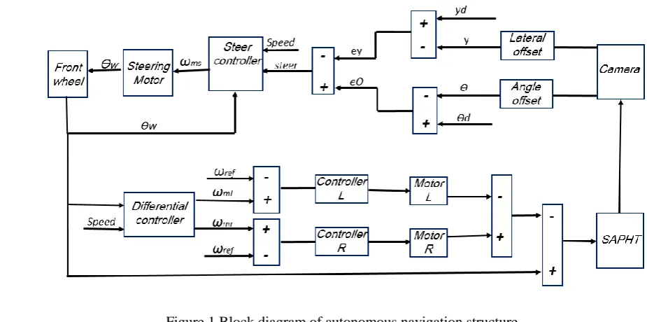
response frequency. As it shown in Figure 1, lateral
offset (y) and angle offset (ϴ) are two parameters
3
Category: Maximum drawbar power of 15-35 kW
extracted from vision system installed on the SAPHT
which are input signals for control structure. These
signals are compared with expected values for lateral
offset (yd) and angle offset (ϴd) for lateral error (ey) and
angle error (eϴ) estimation. The controller also takes the
propelling speed into account to adjust the steering
sensitivity and sends proper order for steering motor
rotation (ωms).
The left front wheel was equipped with a rotational
potentiometer to fed-back turning information (ϴw) into
the closed-loop steering control. The designed system
has a wide range of sensitivity with a resolution of
approximately 0.29 degrees per step.
The potentiometer on the front wheel also sends a
signal for differential controller which controls the speed
of both left and right propelling motors (ωml and ωmr)
in turns and causes accurate navigation of vehicle.
Modelling and simulation of the controller at MATLAB
Simulink with P, PI and PID strategies resulted to
choose PID type controller as the most suitable strategy
due to its ability to eliminate the error and retain on the
path. The results for PID control scheme was proved to
be satisfactory having chosen suitable parameters for
gain coefficient (Kp), integral coefficient (Ki) and
150 September, 2015 Agric Eng Int: CIGR Journal Open access at http://www.cigrjournal.org Vol. 17, No. 3 derivative coefficient (Kd). From numerous
experimental and simulation test results, values of 320,
350 and 40 respectively for Kp, Ki and Kd indicated the
best response. Also, it was found that the P control
creates a steady state error and changing the P control
Kp is not able to eliminate this error. In PI control
mode, although the steady state error is completely
eliminated, its overshoot and settling time will not be
able to satisfy the aim of the design either. However,
the nonlinear control methods are usually quite complex
in applications and the computation effort is too large to
be executed on an economic micro-controller in
real-time applications (Chwa, 2010).
In order to send emergency commands such as force
stop as well as controlling parameters like speed and
steering in teleoperation mode, one remote control
device was developed and tested.
2.2 Navigation algorithm based on machine vision
For machine vision based navigation, a standard
industrial CCD camera (EyeVision EYE-700P-IRIR)
was mounted in front of the SAPHT. Camera setting
was: pitch, roll and yaw angles of 30o, 0o and 0o
respectively at a height of 1.3 m from the ground (Figure
2). The focal length of the lens was 3.5-8 mm and the
data were imported to a laptop using standard LAN port.
The on-board PC on the SAPHT was a personal laptop
with 1 GB installed memory (RAM) and 1.8 GHz
processor that operated under Windows 7 ultimate 32-bit
OS. Since in machine vision mode, online navigation
by means of machine intelligence is required, the images
must be processed on-the-go. So a robust and dynamic
algorithm is required for accurate and agile navigation.
An application program was developed in Visual C#
environment for this purpose. First of all this program
receives video streams using RTSP (Real Time
Streaming Protocol) and plays it on the developed
graphical user interface (GUI) with frame rate of 25 fps.
Then each frame is digitalized and converted to a 24-bit
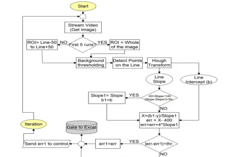
RGB4 color space image. As illustrated in the Figure 3,
for first five images the algorithm seeks for plant rows in
whole of the image (800 * 600 Pixels) as Region of
Interest (ROI). To accelerate the algorithm, after five
frames the ROI box becomes dynamic. The width of
this trapezoidal box is equal to 100 pixels; 50 pixels right
and 50 pixels left the target line (Figure 2). In other
words in the five first image the algorithm searches all
the pixels to find a line with the same color in the image
and after it finds, just seeks around of the line for the rest
of images. Depending on outdoor illumination the
background lighting was varied, so for each frame,
average brightening of pixels inside the ROI area was
redefined as a threshold to find the line in next images.
Line detection method in different condition needs a
factor depending on the color characteristics of each
pixel on the line. As an example for extracting a white
line inside the black background 0.3*R + G/2 can extract
the white pixels accurately where R and G are red and
green matrix of the image in RGB color space
respectively but kG-R-B is a suitable factor for
extraction of green plants rows which k is a coefficient
that varies between 1-2.5 depending on light,
background and plant circumstances. All the pixels
inside the ROI area was compared with the threshold
value and the pixel more than threshold value was set as
the probable points that the line can lie on them. The
main stage of this algorithm was line fitting to
determined points (the right blue line in the Figure 2b).
This task was performed using RHT that is not sensitive
for outliers. Since there were more than one row in
each image so according to distances between rows and
lines slope, the line inside a particular area was selected
as reference foe guidance system. These parameters
may vary from field to field based on planter setting and
need to be set for each field.
4
Although the HT is a robust method for line fitting but it can’t satisfy online demand in robots. To solve
this problem, RHT method using line slope was used.
In this method some points among all detected points
were selected randomly and line was fitted on them
using HT by considering the slope of the last fitted line.
In other words, RHT fits the line on some random points
instead of all of the points but considering the slope of
the line for avoiding any mistake in line fitting. This
method acted five times faster than HT method and
speeded line detection up to 0.2 second without
decreasing accuracy significantly. Figure 3 shows the
flowchart of the line detection and navigation algorithm. Figure 2 The SAPHT in the test course (a), developed line detection program interface (b).
September, 2015 Agric Eng Int: CIGR Journal Open access at http://www.cigrjournal.org Vol. 17, No. 3 152 Two main features of the line; slope and intercept
were extracted for calculation of offset and heading
errors. The slope of straight line was 90o and
acceptable slope range was between 40o and 140o. Also
the absolute value of slopes in two consecutive frames
would not be more than a special threshold depending on
the field characteristics and forward speed. The offset
error was calculated as the departure from the desired
path. Without applying slope impact on the offset error
the vehicle fluctuates in the high speeds. So according
to the given flowchart, final error was derived after
applying slope effect on it. The effect of slope was
applied by ratio of four that was determined
experimentally. Considering vehicle speed, two
consecutive errors would not be more than a predefined
threshold. Finally for correction of steering wheels,
error value flows to the ECU via RS232 interface using a
USB to RS232 converter. At each iteration, some data
include time, offset error, heading and steering signals
were saved in an excel file. Although the algorithm can
be updated by a frequency of 10 Hz, sending data to
ECU decreases the speed and finally the steer was
refreshed by frequency of 3 Hz approximately.
2.3 Experimental evaluation
The designed system was evaluated by comparison
of navigation results in three different modes:
teleoperation, machine vision and manually guidance.
Experimental evaluations were performed in a standard
test course that is provided by the American Society of
Agricultural and Biological Engineers (ASABE) titled as
X587 Dynamic Testing of Satellite-Based Positioning
Devices Used in Agriculture (ASABE, 2007). Due to
existed limitations in campus dimension, the standard
was applied with some changes. Standard X587
provides two straight segments each 90 m long, that
linked by a turn of radius 5-10 m, traveling speeds of 0.1,
2.5, and 5 m/s, test durations of under an hour, and four
repetitions per combination of speed and direction.
Considering dimension of the test campus, two straight
lines each by 40 m length that were linked by a turn of 5
m were sketched using white color (Figure 4). These
tests were performed from March to July 2014 under
different condition of illuminations.
To evaluate the accuracy of designed system based
on machine vision, and to measure the offset drift, the
SAPHT was navigated on the sketched lines as
hypothetical plant rows. In this mode offset from
desire path were measured as an error in four different
speeds: 2, 2.5, 3 and 4 km/hr, each with three
replications. Increasing speed of more than 4 km/hr
leads to miss the line due to fast changes in the direction
and slope, especially in curved tracks due to hardware
slowness. The response frequency of steering system
was evaluated by shifting it from 1 Hz to 3 Hz as well in
speeds of 3 and 4 km/hr. A user interface is developed
in visual C# for video streaming and images are
processed for real-time data mining. The developed
program extracts offset and heading errors from desired
path and sends these data to controller.
Evaluation in teleoperation mode was performed in
the same test course as well. In this mode, the accuracy
was not acceptable for speeds above 2 km/hr (e.g. in 4
km/hr the vehicle fluctuated by maximum error of one
meter approximately). Therefore, the travelling speed
was limited to 2 km/hr, but in three different positions: 1)
two meters far from the corner of the field by
approximately two meter in height, 2) from the center of
the field, and 3) 10 meters far from the center of the field
by approximately five meters in height. The SAPHT
speed was accurately read by an encoder on the drive
wheel. Offset data was extracted in teleoperation mode
using another digital CCD color camera. This camera
saves video from course information and data was
extracted offline. Another application program was
developed in Visual C# environment for this data mining
that was based on HT.
At the end an actual corn field was cultivated in
rows with 90 cm space between them in July of 2014
Figure 4 shows satellite view of test course and field in
the university.
Figure 4 Satellite view of 1) standard test course 2) corn field
Evaluation in manual mode (driver in-the cab) was
performed as well, for comparison. In the manual
mode, the travel speed was set to 2, 4 and 6 km/h, with
three replications for each speed.
To compare the accuracy of each experimental test,
offset and heading errors were calculated in straight and
turning paths separately. The test variables were
different navigation modes, different speeds and steering
system frequency. ANOVA analyses were performed
using the well-known statistical software SPSS V17. 5.
3 Results and discussion
Evaluation tests were carried out in various modes
and speeds between 2 and 4 km/h. To compare the
error of navigation system in straight path and also in the
curved test track, all data were separated in two lines and
turning data categories that respectively refers to straight
path and curved test track. Then, all data were
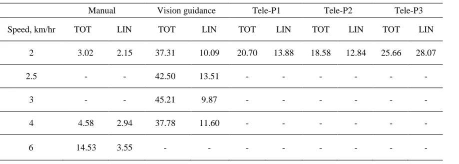
classified in Microsoft Excel before analysis. Table 1
shows a summary of test planning and Root Mean
Square Error (RMSE) of extracted data obtained from
combination of all replications. According to this table
in machine vision mode, the RMSE of straight line (LIN)
was obviously smaller than the RMSE of total path
(TOT) that includes straight and curved path (10.09 cm
versus 37.31 cm). In comparison to teleoperation,
navigation in vision mode had a better performance in
straight paths, while in total path (sum of curved and
straight path), the teleoperation resulted better. In other
word machine vision navigation was followed by the
straight paths accurately but unlike teleoperation mode it
had difficulties in following the curve paths. These
results also showed that the performance of vision mode
in straight path was better than teleoperation mode both
in full path and straight path. This result was completely
expected due to HT conception. The HT which is the
basic concept of the navigation algorithm in this research
is applicable for line detection but it’s not suitable for
fitting line on a curve. On curve path, algorithm needs
another method to detect the path. Increasing the offset
error on curve path resulted from the weakness of HT
and it’s obvious in table results as well as Figure 6.
However curve test tracks in this research were
interpreted as headland turnings which are negligible
compared with row guidance for control system.
Table 1 Test planning and RMSE (cm) of evaluated experiments
Manual Vision guidance Tele-P1 Tele-P2 Tele-P3
Speed, km/hr TOT LIN TOT LIN TOT LIN TOT LIN TOT LIN
2 3.02 2.15 37.31 10.09 20.70 13.88 18.58 12.84 25.66 28.07
2.5 - - 42.50 13.51 - - - -
3 - - 45.21 9.87 - - - -
4 4.58 2.94 37.78 11.60 - - - -
September, 2015 Agric Eng Int: CIGR Journal Open access at http://www.cigrjournal.org Vol. 17, No. 3 154 The SPSS software was used for comparison
of the obtained RMSE’s and assessment of
significance of differences. Analyzing the manual
mode was performed in SPSS software by Duncan
method at the 0.05 level and with speeds of 2, 4 and
6 km/hr. The results indicated that differences
between replications were not significant but there
were significant differences between various speeds
in both full path as well as straight path. For full
path the differences between speeds of 2 km/hr and
4km/hr was nonsignificant while speeds of 2 km/hr
and 4 km/hr had significant difference with 6 km/hr.
The Least Significant Difference (LSD) method had
the same results for full path. However in straight
paths while there was no significant difference
between various speeds by Duncan method, the
difference between 2 km/hr and 6 km/hr was
significant by LSD method.
In the machine vision mode, tests were started by
speed of 2 km/hr and steering frequency of 1 Hz. The
test was continued by the speed of 2.5 km/hr at the same
frequency. Since offset error increased quickly,
consequent tests were continued by increasing the
steering frequency to 3 Hz, at the speed of 3 km/hr.
The last stage is performed by the speed of 4 km/hr and
in steering frequency of 3 Hz.
Statistical analyses in vision mode illustrated
significant differences due to steering frequency. It’s
concluded that the frequency has an important effect on
system performance. According to Duncan test in full
path there was no significant difference between various
speeds while differences in straight paths were
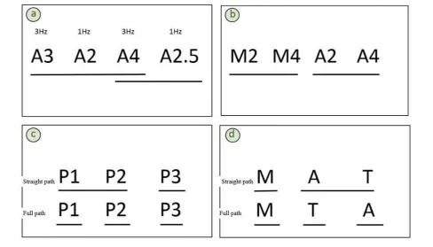
significant. Figure 5 shows the summary of results
extracted from mean comparison for vision mode. In
this figure letter ‘V’ refers to vision mode and
subscripted numbers indicates the speed of vehicle.
The line under the letters divides the symbols in different
subsets which means the modes with same underline
belong to the same subset and the difference between
them is not significant. The results are arranged from
good to bad at each figure. As illustrated in the Figure 5a,
V3 gives best result which means that high frequency in
low speed leads to accurate navigation. The V2.5 with
travelling speed of more than V2 and in the same
frequency had worst result which confirmed the
frequency and speed impact on control process. As is
shown, differences between V2 and V4 and also V4 and
V2.5 were not significant. This result could be
interpreted as the importance of steering system
frequency in vision based navigation. Due to the
impact of steering frequency, the V4 with the highest
travel speed had no significant difference with V2 that
had the lowest speed.
To compare machine vision mode versus manually
driving, an analysis was performed between V2, V4, M2
and M4 (‘M’ refers to Manual mode and subscripted
numbers show the travel speed). The results illustrated
that the differences between machine vision mode and
Manual mode was significant at 0.01 levels with the
predominance of manual mode (Figure 5b).
Teleoperation mode was evaluated from three
different positions (P1, P2 and P3). As is shown in
Figure 5c, in straight path there was significant
difference at 0.01 levels between P3 and two other
positions. As P2 refers to the center of the course, it is
concluded that this difference was resulted from the
distance between operator and vehicle. When operator
stands in a far distance from the vehicle, due to optical
illusions a biased error occurred from the desired path.
However, analysis in full path and based on Duncan test,
illustrates that three positions had significant difference
Finally three different modes were compared in a
constant speed of 2 km/hr (Figure 5d). Results of
analysis indicated that differences between three modes
were significant in full path at 0.05 levels. In full path
the performance of Teleoperation mode was better than
vision mode but worse than Manual mode. While in
straight path the performance of vision mode was better
but the difference was not significant. The Manual
mode had significant differences with vision mode and
Teleoperation mode in both full path as well as straight
path.
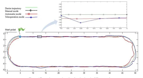
Figure 6 shows test trajectory and results of
evaluations in different modes. In this figure the
desired test trajectory is shown by green line and the best
replication of traveled routes in speed of 2 km/hr are
illustrated by different colors and symbols. According
to this figure in straight path vision navigation
(red-square) follows the straight path accurately but
encounters gross error in turning curved track. Figure 5 Mean comparison result of RMSE in different modes
156 September, 2015 Agric Eng Int: CIGR Journal Open access at http://www.cigrjournal.org Vol. 17, No. 3
As illustrated in Figure 6, and also according to the
results of RMSE comparison, Teleoperation mode gives
good results in turning curves in comparison to vision.
However in straight paths that are more susceptible for
agricultural fields the accuracy of vision based
navigation is favorable. Overall, comparing two
evaluated methods for navigation between field rows, the
machine vision has remarkable predominance.
However, application of a combination of two evaluated
modes would be affordable for a successful navigation.
Between rows that crop line is detectable, the vision
system could handle accurately, while in headland
turnings that there is no guidance sign, teleoperational
control would give good results, especially if the control
is performed from a Graphic User Interface (GUI) in the
farm office.
SAPHT was passed 25 meter straight path between
rows in actual field without hurting any corn with RMSE
of about 5.7 cm. Travelling speed in this test was set to
2 km/h but excessive distance between corns (more than
50 cm) and also weakness of some corns as it’s apparent
in Figure 2b caused failure in the algorithm. Extracted
data from 25 m path were showed 1.7 cm mean error.
Astrand et al. (2005) tested a row following robot with
the speed of 0.1 m/s which could pass a 36 m path with
maximum error of 2.3 cm (Åstrand and Baerveldt, 2005).
However increasing speed and accuracy of a row
following robots need more and more researches. Row
plan also has an important effect on the guidance quality
that should be noticed.
4 Conclusion
Automatic navigation is one of the sophisticated tasks
that were under consideration over the last century. To
obtain a full automatic vehicle that can be applicable in
the straight rows and headland turning, an autonomous
system was developed and evaluated in three different
modes (machine vision, teleoperation and manually).
The study was implemented on actual sized platform,
titled as Solar Assist Plug-in Hybrid electric Tractor
(SAPHT). Experimental evaluations were conducted
with various speeds, different steering frequency and
several positions for teleoperation mode. Offset and
heading errors were extracted using RHT and dynamic
thresholding in each images. Test results were
curved test track. RMSE analysis in the straight path
illustrated the prominence of vision based guidance
(10.09 cm). While in the turning curves;
teleoperational navigation showed good results (12.84
cm). However curve test track interpreted as headland
turning which is negligible compared with row guidance.
Test results indicated that increasing movement velocity
increased the offset error and steering frequency had
important impact on the navigation accuracy. However,
for an accurate navigation, combination of the two
evaluated methods would be recommended, i.e. between
rows that crop line is detectable, vision system could
handle accurately, while in turning path that there is no
guidance sign, teleoperational control would perform
properly, especially if the control is performed from a
GUI in the farm office.
Acknowledgment
The financial support provided by the University of
Tehran under grant number 73130963/1/01, Iran, is duly
acknowledged.
References
ASABE 2007. X587 Dynamic Testing of Satellite-Based Positioning Devices used in Agriculture. St. Joseph, ASABE.
ÅSTRAND, B. & BAERVELDT, A.-J. 2005. A vision based row-following system for agricultural field machinery. Mechatronics, 15(2), 251-269.
CHWA, D. 2010. Tracking control of differential-drive wheeled mobile robots using a backstepping-like feedback linearization. IEEE Transactions on Systems, Man and Cybernetics, Part A: Systems and Humans, 40(6), 1285-1295.
ENGLISH, A., ROSS, P., BALL, D. & CORKE, P. Vision based guidance for robot navigation in agriculture. Robotics and Automation (ICRA), 2014 IEEE International Conference on, 2014. IEEE, 1693-1698.
J. BILLINGSLEY , M. S. 1997. The successful development of a vision guidance system for agriculture. Computers and Electroncis in Agriculture
16(2), 7.
JI, R. & QI, L. 2011. Crop-row detection algorithm based on Random Hough Transformation. Mathematical and Computer Modelling, 54(3), 1016-1020.
JIANG, H., XIAO, Y., ZHANG, Y., WANG, X. & TAI, H. 2013. Curve path detection of unstructured roads for the outdoor robot navigation. Mathematical and Computer Modelling, 58(3-4), 536-544.
LEEMANS, V. & DESTAIN, M. F. 2006. Application of the Hough Transform for Seed Row Localisation using Machine Vision. Biosystems Engineering, 94(3), 325-336.
MONTALVO, M., PAJARES, G., GUERRERO, J. M., ROMEO, J., GUIJARRO, M., RIBEIRO, A., RUZ, J. J. & CRUZ, J. M. 2012. Automatic detection of crop rows in maize fields with high weeds pressure. Expert Systems with Applications, 39(15), 11889-11897.
MOUSAZADEH, H., KEYHANI, A., JAVADI, A., MOBLI, H., ABRINIA, K. & SHARIFI, A. 2011. Life-cycle assessment of a Solar Assist Plug-in Hybrid electric Tractor (SAPHT) in comparison with a conventional tractor. Energy Conversion and Management, 52(3), 1700-1710.
PINTO, F. A. C., REID, J. F., ZHANG, Q. & NOGUCHI, N. 2000. Vehicle Guidance Parameter Determination from Crop Row Images using Principal Component Analysis. Journal of Agricultural Engineering Research, 75(3), 257-264.
TANGWONGKIT, R., SALOKHE, V. & JAYASURIYA, H. 2006. Development of a Tractor Mounted Real-time,Variable Rate Herbicide Applicator for Sugarcane Planting. Agricultural Engineering International: the CIGR Ejournal, VIII.
TILLETT, N. 1991. Automatic guidance sensors for agricultural field machines: a review. Journal of agricultural engineering research, 50, 167-187.
TILLETT, N., HAGUE, T. & MILES, S. 2002. Inter-row vision guidance for mechanical weed control in sugar beet. Computers and Electronics in Agriculture, 33(3), 163-177.
TONY , G., QIN , Z., NAOSHI , K. & KC , T. 2008. A review of automation and robotics for the bio-industry. Journal of Biomechatronics Engineering, 1(2), 37-54.
WU, X., XU, W., SONG, Y. & CAI, M. 2011. A Detection Method of Weed in Wheat Field on Machine Vision. Procedia Engineering, 15, 1998-2003.
XUE, J. 2014. Guidance of an agricultural robot with variable angle-of-view camera arrangement in cornfield. African Journal of Agricultural Research, 9(18), 1378-1385. XUE, J. L. & GRIFT, T. E. Agricultural Robot Turning in the
Headland of Corn Fields. Applied Mechanics and Materials, 2011. Trans Tech Publ, 780-784.
158 September, 2015 Agric Eng Int: CIGR Journal Open access at http://www.cigrjournal.org Vol. 17, No. 3
Abbreviations:
3PH Three Point Hitch
ASABE American Society of Agricultural and Biological Engineers
CCD Charge Coupled Device
CVT Continuous Variable Transmission ECU Electronic Control Unit
PGS Global Positioning System GUI Graphic User Interface
HT Hough Transform Ki Coefficient of Integral
Kp Coefficient of Proportional
Kd Coefficient of Derivative
M Manual mode
P Position PTO Power Take Off PV Photovoltaic
RGB Red-Green-Blue color space RHT Randomized Hough Transform RMSE Root Mean Square Error ROI Region of Interest
SAPHT Solar Assist Plug-in Hybrid electric Tractor T Teleoperation mode