Regionally refined test bed in E3SM atmosphere model version 1 (EAMv1) and applications for high-resolution modeling

(1)

Geosci. Model Dev., 12, 2679–2706, 2019 https://doi.org/10.5194/gmd-12-2679-2019 © Author(s) 2019. This work is distributed under the Creative Commons Attribution 4.0 License.

Regionally refined test bed in E3SM atmosphere model version 1

(EAMv1) and applications for high-resolution modeling

Qi Tang1, Stephen A. Klein1, Shaocheng Xie1, Wuyin Lin2, Jean-Christophe Golaz1, Erika L. Roesler3, Mark A. Taylor3, Philip J. Rasch4, David C. Bader1, Larry K. Berg4, Peter Caldwell1, Scott E. Giangrande2, Richard B. Neale5, Yun Qian4, Laura D. Riihimaki4, Charles S. Zender6, Yuying Zhang1, and Xue Zheng1 1_{Lawrence Livermore National Laboratory, Livermore, CA 94550, USA}

2_{Brookhaven National Laboratory, Upton, NY 11973, USA} 3_{Sandia National Laboratory, Albuquerque, NM 87185, USA} 4_{Pacific Northwest National Laboratory, Richland, WA 99352, USA} 5_{National Center for Atmospheric Research, Boulder, CO 80305, USA}

6_{Departments of Earth System Science and Computer Science, University of California,} Irvine, Irvine, CA 92697, USA

Correspondence:Qi Tang ([email protected])

Received: 14 January 2019 – Discussion started: 6 February 2019

Revised: 15 May 2019 – Accepted: 12 June 2019 – Published: 8 July 2019

Abstract. Climate simulations with more accurate process-level representation at finer resolutions (<100 km) are a pressing need in order to provide more detailed actionable information to policy makers regarding extreme events in a changing climate. Computational limitation is a major obsta-cle for building and running high-resolution (HR, here 0.25◦ average grid spacing at the Equator) models (HRMs). A more affordable path to HRMs is to use a global regionally refined model (RRM), which only simulates a portion of the globe at HR while the remaining is at low resolution (LR, 1◦). In this study, we compare the Energy Exascale Earth Sys-tem Model (E3SM) atmosphere model version 1 (EAMv1) RRM with the HR mesh over the contiguous United States (CONUS) to its corresponding globally uniform LR and HR configurations as well as to observations and reanalysis data. The RRM has a significantly reduced computational cost (roughly proportional to the HR mesh size) relative to the globally uniform HRM. Over the CONUS, we evaluate the simulation of important dynamical and physical quantities as well as various precipitation measures. Differences between the RRM and HRM over the HR region are predominantly small, demonstrating that the RRM reproduces the precipita-tion metrics of the HRM over the CONUS. Further analysis based on RRM simulations with the LR vs. HR model pa-rameters reveals that RRM performance is greatly influenced

by the different parameter choices used in the LR and HR EAMv1. This is a result of the poor scale-aware behavior of physical parameterizations, especially for variables influenc-ing sub-grid-scale physical processes. RRMs can serve as a useful framework to test physics schemes across a range of scales, leading to improved consistency in future E3SM ver-sions. Applying nudging-to-observations techniques within the RRM framework also demonstrates significant advan-tages over a free-running configuration for use as a test bed and as such represents an efficient and more robust physics test bed capability. Our results provide additional confirma-tory evidence that the RRM is an efficient and effective test bed for HRM development.

1 Introduction

(2)

parameteri-2680 Q. Tang et al.: Regionally refined test bed in E3SM atmosphere model version 1 zations are important steps of model development. However,

the computational cost of running a globally uniform HR model (HRM) is high. For example, a 1-year 0.25◦_{HR E3SM}

atmosphere model version 1 (EAMv1) simulation requires 0.6 million core hours on 675 “Knights Landing” (KNL, In-tel Xeon Phi Processor 7250) nodes of the Cori supercom-puter at the National Energy Research Scientific Computing Center (NERSC). A regionally refined model (RRM) capa-bility (Ringler et al., 2008; Zarzycki and Jablonowski, 2014; Roesler et al., 2019), which only simulates a fraction of the globe at HR, is adopted by EAMv1 to reduce the computa-tional cost of HR simulations and to examine the parameter-ization sensitivity to HR scales. The RRM simulation cost is usually dominated by the computational cost of the HR re-gion, and thus the total model cost is roughly proportional to the size of the region with finer resolution, referred to as a “mesh” (typically chosen to be about 10 % of the globe, mak-ing the cost about 10 % of a uniform HRM simulation). In the ongoing E3SM phase II project, the RRM configuration is planned as a central tool to achieve the E3SMv2 science goal of understanding the relative impacts of global forcing versus regional influences of human activities on flood and drought in North America. RRM will be routinely used over North America to address DOE’s goal of understanding the Earth system changes affecting US energy-sector decisions. It will be also applied as a physics test bed to improve the scale awareness of parameterizations in upcoming versions of E3SMv2 and v3 as well as an important strategy to per-form a larger ensemble of HR simulations. RRM is also a vi-tal capability for progress towards an eventual global cloud-resolving model with 3 km horizontal grid spacing targeting E3SMv4 and beyond.

The RRM approach has been established and validated with other models over many regions of interest. For in-stance, Zarzycki et al. (2014) showed the effectiveness of an RRM with aquaplanet experiments using the Community At-mosphere Model (CAM). Zarzycki and Jablonowski (2014, 2015) demonstrated improved skill in simulating tropical cyclones in CAM with a refined mesh over the North At-lantic. Rhoades et al. (2016) and Wu et al. (2017) depicted that the variable-resolution (VR) Community Earth System Model (CESM) was able to accurately capture the clima-tology and seasonality of important variables over moun-tain regions. Huang and Ullrich (2017) reproduced the ge-ographic patterns of historical precipitation climatology over the western US with the VR-CESM. Gettelman et al. (2018) performed comprehensive tests of a VR dynamical core in CESM2 and showed that VR grids were feasible alternatives to conventional nesting for regional climate research. Roesler et al. (2019) found that refining the grid over the contiguous United States (CONUS) did not exert a noticeable influence on the global circulation in the EAM version 0 (EAMv0, which is almost identical to CAM5.3 except for some mi-nor tunings and bug fixes). These earlier studies have demon-strated that RRMs can be used as an effective tool to study

important climate features over regions of interest with high resolution.

Compared to EAMv0, EAMv1 (Rasch et al., 2019) cludes significant changes to its physics, substantially in-creased vertical resolution, retuning, and bug fixes (Zhang et al., 2018). All these changes cause the model to behave very differently from EAMv0, especially in terms of regional clouds and precipitation characteristics (Xie et al., 2018). Given these substantial model changes and the critical role that RRM will play in future E3SM scientific applications, this paper documents further scientific analysis of RRM be-havior with EAMv1. We contrast simulations between the RRM and the globally uniform HR EAMv1 over the RRM region, with the goal of providing more insights into the EAMv1 RRM capability to the user community. This study emphasizes hydrology-related simulation skill over North America: a key element of the E3SM Water Cycle science driver. We investigate whether RRM reproduces the same performance as HRM of these fields enabling it to be used as an effective physics test bed for understanding physical processes and improving their representations in EAMv1 and in future versions. In addition, EAMv1 physical parameter-izations (and in particular the cloud parameterparameter-izations) are not inherently scale-aware and hence require retuning when increasing model horizontal or vertical resolution. Unfor-tunately, this leads to two different parameter settings for EAMv1 high- and low-resolution models. It is key to de-termine how the two different parameter settings influence RRM performance, since most earlier studies just used the established low-resolution model parameters over the RRM domain, which may not yield optimal RRM results due to scale-aware shortcomings of the existing physical schemes.

This study centers mainly on “proof-of-concept” exam-ples. More in-depth analysis of RRM behavior will be re-ported in separate studies when RRM is more routinely used in E3SM phase II and by general users. In many EAMv1 application scenarios, it is expected that the RRM will be more feasible and practical than the HRM. This could in-clude evaluation against regional measurements, uncertainty quantification studies that typically demand a large ensemble size (Qian et al., 2016, 2018), and users with limited com-putational resource. Findings from this study regarding the strengths and weaknesses of the EAMv1 RRM configuration should provide valuable guidance for future RRM applica-tions in the HR E3SM development and broad community use of the E3SM RRM.

(3)

Q. Tang et al.: Regionally refined test bed in E3SM atmosphere model version 1 2681 et al. (2012) and Ma et al. (2014) demonstrated a strong

cor-respondence between short (a few days) and long (seasonal to annual) timescale systematic errors in climate models for fields related to fast physics, such as clouds and precipitation. This paper is organized as follows. Section 2 provides an overview of the RRM EAMv1 and summarizes the setup of simulations and the observational datasets used for model evaluation. Results are shown in Sect. 3, including model cli-matologies over the CONUS domain where our RRM has its fine-resolution mesh, the analysis of quantities related to the hydrological cycle, and an in-depth analysis of precipitation characteristics – the large-scale to convective partitioning, the intensity distribution, and the summertime diurnal cycle. Section 4 describes an example of running the nudged RRM. Section 5 provides a summary of this work and prospects for future studies.

2 Methodology

2.1 Model overview and experiment design

The E3SM project aims to build a global HR fully cou-pled Earth system model for climate simulation and predic-tion on current and next-generapredic-tion supercomputing facili-ties (Bader et al., 2014). Since all the simulations analyzed here are atmosphere-only ones, we only provide informa-tion about the atmosphere model. Details about the coupled E3SM model can be found in Golaz et al. (2019). EAMv1 originated from CAM5.3 (Neale et al., 2012) but has un-dergone substantial development. An overview of EAMv1 is given by Rasch et al. (2019). More details on the sim-ulated cloud and precipitation characteristics and overview of the low- and high-resolution model tunings are provided in Xie et al. (2018). EAMv1 uses the spectral element dy-namical core (Taylor and Fournier, 2010; Dennis et al., 2012) on a cubed-sphere computation grid with an explicit Runge– Kutta time integration scheme. This dynamical core has sus-tained scalability with an increasing number of elements and processors (Fournier et al., 2004). Major changes in EAMv1 compared to its earlier version include substantially increased vertical resolution (72 vs. 30 vertical layers), a higher (∼0.1 hPa compared to 2 hPa) model top, and im-proved physical parameterizations including the Cloud Lay-ers Unified By Binormals (CLUBB) scheme (Golaz et al., 2002; Bogenschutz et al., 2013), updated cloud microphysics (MG2) (Gettelman and Morrison, 2015), predicted aerosols (the Modal Aerosol Module, MAM4) (Liu et al., 2016), and a linearized ozone chemistry (Linoz2) (Hsu and Prather, 2009). Impacts of the new cloud physics and the increase in vertical resolution on EAMv1-simulated climate are documented in Xie et al. (2018) and Qian et al. (2018). In the present paper, we focus on the EAMv1 regionally refined test bed capability over the CONUS domain.

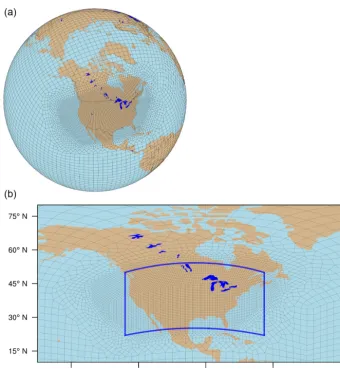
The CONUS regionally refined grids consist of LR and HR regions and a transition area between them (see Fig. 1a). The HR grid is located in the CONUS area. We created the regionally refined grid with the offline software tool Spheri-cal Quadrilateral Grid Generator (SQuadGen, https://github. com/ClimateGlobalChange/squadgen, last access: 14 May 2019). The effective resolutions for the LR and HR regions are 1 and 0.25◦, respectively. Because of the horizontal res-olution differences in the low-resres-olution model (LRM), the HRM, and the RRM, the topography is represented differ-ently in these configurations. We used a new tensor hypervis-cosity formulation (Guba et al., 2014) to eliminate numerical noise and oscillations. Additional details about the CONUS RRM as well as the topography data are reported in Roesler et al. (2019). It is worth mentioning that the RRM grids have also being generated and tested over the tropical western Pa-cific (TWP) and the eastern North Atlantic (ENA).

In the present study, we mainly analyze the atmosphere-only simulations (see Tables 1 and A1) forced by observed present-day climatologies of aerosol emissions, greenhouse gases, sea surface temperatures (SSTs), and sea ice concen-trations. The simulations use an interactive E3SM land model on the same grids as the atmosphere. We run the EAMv1 with globally uniform LR and HR grids as well as the CONUS RRM grid. All simulations are performed with the 72 verti-cal layers. Since the EAMv1 parameterizations are not sverti-cale- scale-aware, both dynamical and physical parameters are adjusted to optimize the model performance at different resolutions (Xie et al., 2018). This leads to different parameter settings for the EAMv1 LRM and HRM. As shown in Table A1 of Xie et al. (2018), the differences are mainly in parameters that control convection and cloud microphysics. Thus, dif-ferences between LRM and HRM analyzed in the following sections arise from different horizontal resolutions and pa-rameter settings as well as the different physics time steps. The LRM and HRM physics time steps are 30 and 15 min, respectively. The dynamics use three layers of substepping. For the LRM (HRM), the Lagrangian vertical discretization time step is 15 min (2.5 min), the horizontal discretization time step is 5 min (75 s), and the explicit numerical diffusion time step is 100 s (18.75 s). The RRM uses the same dynam-ics time steps over the LR and HR domains. For the purpose of mimicking the HRM behaviors, we opt to use the same dy-namical and physical parameters and time step for the RRM control simulation as in the HRM. Besides the RRM con-trol case, we also perform an RRM test (RRM_LR) with the LRM dynamical and physical parameters. Comparing these two RRM results, we are able to explore the impact of dif-ferent parameter settings on the RRM performance, which is not possible for conventional RRM studies with only the LR parameters.

(4)

2682 Q. Tang et al.: Regionally refined test bed in E3SM atmosphere model version 1

Figure 1.The CONUS regionally refined grid in(a)a global orthographic projection and(b)a cylindrical equidistant projection zoomed in over the high-resolution (HR) portion. The effective resolutions for the low-resolution (LR) and the HR regions are 1 and 0.25◦, respectively. The two regions are connected with a transient area. The blue box (latitude range: 22–50◦N, longitude range: 64–126◦W) in panel(b)

represents the analyzed area for CONUS.

Table 1.List of EAMv1 simulation configurations, speed, and costs. The speed and cost are for the NERSC Cori-KNL machine. SYPD: simulation year per day.

Simulation Configuration Effective angular Number of Speed Number of Cost

(core-resolution elements (SYPD) nodes hours per year)

Low-resolution model (LRM) Default 1◦ 5400 6 81 22 000

High-resolution model (HRM) Default 0.25◦ 86 400 2 675 551 000

Regionally refined model (RRM) HRM default 1 to 0.25◦ 9905 1.7 88 84 000

RRM_LR LRM default 1 to 0.25◦ 9905 1.9 88 75 000

LRM AMIP Default 1◦ 5400 6 81 22 000

RRM non-US nudging HRM default 1 to 0.25◦ 9905 1.7 88 84 000

compensating errors from nonlinear feedback mechanisms also contribute to climate mean biases, making it a challenge to pin the errors to specific parameterizations. The numeri-cal weather prediction technique (Phillips et al., 2004), also known as the transpose Atmospheric Model

(5)

Q. Tang et al.: Regionally refined test bed in E3SM atmosphere model version 1 2683 RRM can be run in a nudging configuration to diagnose

parameterization-related errors and help to guide develop-ment in HR E3SM. More guidance on using the nudged RRM approach will be discussed in Sect. 4.

To demonstrate the nudging capability, we perform an RRM simulation nudged to the European Centre for Medium-range Weather Forecasting Interim (ERAI) analysis fields of horizontal velocities (U andV) (Dee et al., 2011) with a 6 h relaxation timescale. The nudged simulation uses the prescribed weekly, 1◦spatial resolution SSTs and sea ice from the National Oceanic and Atmospheric Administration Optimum Interpolation analysis data (Reynolds et al., 2002). In addition, we conduct an LR atmosphere-only simulation with time-evolving forcings (i.e., AMIP style) to compare it with the nudging simulation. Output from the Cloud Feed-back Model Intercomparison Project Observation Simulator Package (COSP) (Bodas-Salcedo et al., 2011) is used to com-pare with cloud observations from satellites (Zhang et al., 2019). All free-running simulations are run for a period of 5 years. The first year is regarded as spin-up; thus, we study the results from the last 4 years. The nudging run simulates the year 2011, whereas the AMIP results are extracted for the year 2011 from a long simulation starting from 1870 (Golaz et al., 2019). Model output is stored as monthly and hourly averages.

2.2 Evaluation datasets

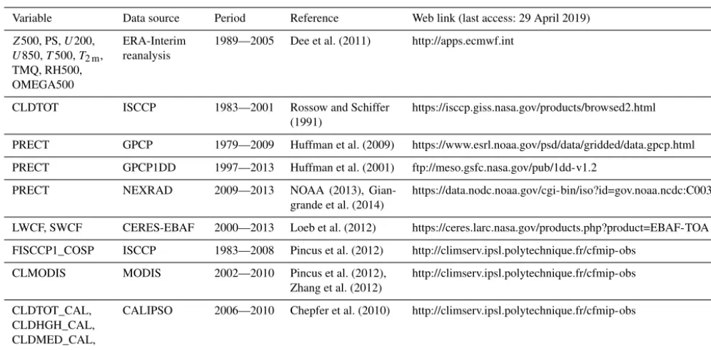
Skillful depictions of the large-scale circulation and sub-grid-scale physics are essential for more realistic model simulations of the atmospheric hydrological cycle. We choose evaluation variables to cover both aspects. Evaluation datasets are summarized in Table 2. Meteorological fields, such as geopotential height, surface pressure, winds, temper-ature, relative humidity, and precipitable water are from the ERAI reanalysis product (Dee et al., 2011). Seasonal pre-cipitation climatology estimations are based on the Global Precipitation Climatology Project (GPCP) (Huffman et al., 2009). Daily precipitation observations are taken from the GPCP 1◦daily (1DD) data (Huffman et al., 2001). Hourly precipitation is compared with the dataset collected by the Next-Generation Radar (NEXRAD) network (NOAA, 2013) and developed under the Climate Science for a Sustainable Energy Future (CSSEF) project (Zhang et al., 2005, 2011; Giangrande et al., 2014). Simulated cloud amount is veri-fied against International Satellite Cloud Climatology Project (ISCCP) data (Rossow and Schiffer, 1991). In order to com-pare with the cloud diagnostics from COSP, we also use the satellite data products generated especially for model evalu-ation from ISCCP (Pincus et al., 2012; Zhang et al., 2012), Moderate Resolution Imaging Spectroradiometer (MODIS) (Pincus et al., 2012), and Cloud-Aerosol Lidar and Infrared Pathfinder Satellite Observation (CALIPSO) (Chepfer et al., 2010). Top-of-atmosphere cloud radiative effects are evalu-ated with the Clouds and the Earth’s Radiant Energy System–

Energy Balanced and Filled (CERES-EBAF v2.8) dataset (Loeb et al., 2012).

3 Results

In this section, we will focus on the results of June–July– August (JJA) and December–January–February (DJF), the two more extreme seasons at the CONUS in a year when some long-standing systematic model errors are present.

3.1 Overall model performance

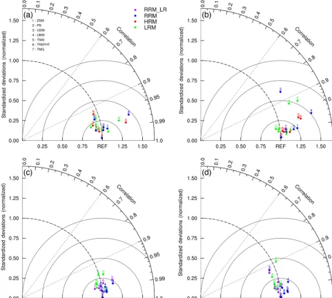
Taylor diagrams (Taylor, 2001) offer a concise way of sum-marizing model performance and comparing different model results. Here we employ Taylor diagrams to demonstrate the performance of a selection of important variables (Gleck-ler et al., 2016). Figure 2 shows the JJA and DJF model climatology of selected thermodynamically related variables (numbered) over the CONUS domain (i.e., the blue box in Fig. 1b) of the RRM grids. Green dots denote LRM results, whereas red dots indicate HRM results and blue dots RRM results with the HRM parameters. The model results are il-lustrated relative to the verification data (marked by the ref-erence point (1, 0)) described in Sect. 2.2. To make consis-tent comparisons between different model resolutions, model results are conservatively interpolated (with the “conserve” method of the Earth System Modeling Framework, ESMF, https://www.earthsystemcog.org/projects/esmf/, last access: 1 May 2019, regridding software) to the coarser verification data grids before calculating the Taylor statistics. The radial axis shows the geographic variability (i.e., standard devia-tion, SD) in the model climatology normalized by that in the observations. The angular axis indicates the spatial cor-relation (i.e., Pearson corcor-relation coefficient,r) between the simulations and the observations. By design, the distance to the reference point (1, 0) represents the centered root-mean-square (rms) difference between the simulated and observed patterns normalized by the SD of the observations. The closer the distance to the (1, 0) point, the better the model perfor-mance. We should note that the primary purpose of our analy-sis is to show how well the RRM, as an analogue to the HRM, reproduces the HRM results. The observations and the LRM results provide quantitative references to examine the RRM– HRM similarity and also identify poorly simulated behaviors as targets of HRM development.

(6)

Table 2.Summary list of observational and reanalysis-based evaluation datasets for model performance.

Variable Data source Period Reference Web link (last access: 29 April 2019)

Z500, PS,U200, U850,T500,T2 m, TMQ, RH500, OMEGA500

ERA-Interim reanalysis

1989—2005 Dee et al. (2011) http://apps.ecmwf.int

CLDTOT ISCCP 1983—2001 Rossow and Schiffer (1991)

https://isccp.giss.nasa.gov/products/browsed2.html

PRECT GPCP 1979—2009 Huffman et al. (2009) https://www.esrl.noaa.gov/psd/data/gridded/data.gpcp.html

PRECT GPCP1DD 1997—2013 Huffman et al. (2001) ftp://meso.gsfc.nasa.gov/pub/1dd-v1.2

PRECT NEXRAD 2009—2013 NOAA (2013), Gian-grande et al. (2014)

https://data.nodc.noaa.gov/cgi-bin/iso?id=gov.noaa.ncdc:C00345

LWCF, SWCF CERES-EBAF 2000—2013 Loeb et al. (2012) https://ceres.larc.nasa.gov/products.php?product=EBAF-TOA

FISCCP1_COSP ISCCP 1983—2008 Pincus et al. (2012) http://climserv.ipsl.polytechnique.fr/cfmip-obs

CLMODIS MODIS 2002—2010 Pincus et al. (2012), Zhang et al. (2012)

http://climserv.ipsl.polytechnique.fr/cfmip-obs

CLDTOT_CAL, CLDHGH_CAL, CLDMED_CAL, CLDLOW_CAL

CALIPSO 2006—2010 Chepfer et al. (2010) http://climserv.ipsl.polytechnique.fr/cfmip-obs

(LRM). Nevertheless, there are a few exceptions, for exam-ple, 2 m air temperature (T2 m or TREFHT, reference height temperature) in JJA (see Fig. 2a), which is likely associated with cloud and thus surface radiation changes (Van Wever-berg et al., 2018) along with feedbacks (surface energy par-titioning shifting towards more sensible heat flux) from the land surface model.

More importantly, when using the HRM as the reference point (Fig. 2c, d), blue dots (RRM) are located closer to (1, 0) than the green dots (LRM), indicating that the RRM mim-ics the HRM behaviors quite well. Additionally, we plot the RRM_LR results (purple dots) on Fig. 2c, d to illustrate the potential impact of poor scale awareness, which is a common problem for current climate models, on conventional RRM applications. Lacking the tuned HRM parameters, previous RRM studies often rely heavily on LRM parameters and can-not quantify the likely performance deterioration due to the parameter–resolution mismatch. Here we take advantage of having both LR and HR tuned parameters to show the param-eter influence on RRM performance. As expected, RRM_LR is generally less satisfactory than RRM in matching the HRM behaviors (Fig. 2c, d), but the extent varies for different quan-tities. For instance, the 200 hPa zonal wind (U200) is rela-tively insensitive to parameter changes in RRM configura-tions in both seasons. These results reflect the large-scale na-ture of upper-troposphere wind fields. In contrast toU200, RRM total precipitable water (TMQ) shows greater sensitiv-ity to parameter settings, since it is more closely related to sub-grid-scale physical processes. These results suggest that RRM generally does well in representing large-scale

thermo-dynamical behaviors of HRM, but some quantities are sensi-tive to the choice of LRM or HRM parameter settings. A re-tuning may be needed for the refined region to optimize per-formance when model physical parameterizations are scale-sensitive. Specifically, for EAMv1, using the HRM parame-ter setting is recommended when one utilizes the RRM capa-bility.

(7)

Q. Tang et al.: Regionally refined test bed in E3SM atmosphere model version 1 2685

Figure 2.Taylor diagrams for three different model climatologies (color-coded: green – LRM; red – HRM; blue – RRM; and purple – RRM_LR) in JJA(a, c) and DJF(b, d). Results are from the CONUS domain (the blue box in Fig. 1b). For panels(a)and(b), verification data are used as the reference point (1, 0), and statistics are calculated on the coarser verification grids. For panels(c)and(d), the HRM is the reference, and statistics are calculated on the HRM grids. The numbers represent the following: 1 – 500 hPa geopotential height (Z500); 2 – surface pressure (PS); 3 – 200 hPa zonal wind (U200); 4 – 850 hPa zonal wind (U850); 5 – 500 hPa temperature (T500); 6 – 2 m air temperature (TREFHT orT2 m); and 7 – total precipitable water (TMQ).

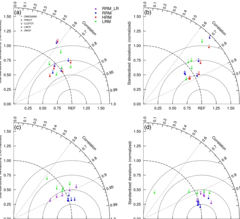
summer (greater LRM–HRM separation in Fig. 3b than in Fig. 3a). For example, the variance of 500 hPa vertical ve-locity (OMEGA500) is almost independent of resolution in summer but about 50 % larger in the HRM configuration than in the LRM in winter, suggesting stronger wintertime circu-lation and a finer scale of resolved dynamics with the HRM configuration.

These overall Taylor statistics indicate that the RRM sim-ulation with the HR parameters captures the HRM climato-logical statistics reasonably well, which provide the basis for

(8)

Figure 3.Same as Fig. 2, but the numbers represent the following: 1 – 500 hPa vertical velocity (OMEGA500); 2 – total precipitation (PRECT); 3 – vertically integrated total cloud fraction (CLDTOT); 4 – longwave cloud forcing (LWCF); and 5 – shortwave cloud forcing (SWCF).

3.2 Regional geographic patterns

In this section we study whether RRMs can reproduce the re-gional geographic patterns of hydrologic variables simulated by HRM.

3.2.1 Precipitation

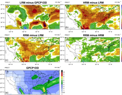
Figure 4 shows the geographic pattern of mean total (large-scale+convective) precipitation differences between LRM and GPCP1DD observations and the differences among model configurations over the CONUS domain in JJA. The differences between the LRM and evaluation data

(9)

Figure 4.Mean differences of total precipitation (unit: mm d−1) in JJA for(a)LRM minus GPCP1DD data,(b)HRM minus LRM,(c)RRM minus LRM,(d)RRM minus HRM, and(e)GPCP1DD. The differences between the LRM and evaluation data (i.e., panela) are computed on the evaluation grid, while those between models (i.e., panelsb–d) are computed on the HRM grid. Dotted areas denote where the differences are statistically significant at the 95 % confidence level with the two-tailed Student’sttest.

over land) among different model configurations (Fig. 4b–d). Over land, the HRM and RRM typically produce less precip-itation than the LRM (partially due to the model tuning, not shown) and the HRM rains the least. Differences between the RRM and the HRM are largely insignificant. In regions that pass the significance test, the differences are also relatively small, for instance, <1 mm d−1in the southern central US and<2 mm d−1in the eastern US.

Figure 5 shows the differences in precipitation climatology patterns for DJF. An obvious change from the JJA results in Fig. 4 is the topographic signatures in differences between HRM and LRM (Fig. 5b) and RRM and LRM (Fig. 5c) over mountain regions in the western US, which are associated with better-resolved topography in the RRM and HRM sim-ulations. In addition, the signs of model differences (Fig. 5b– d) are less uniform in DJF than in JJA. Nevertheless, mean

precipitation differences between the RRM and the HRM are also small (within±2 mm d−1_{) and not statistically} sig-nificant over most grid cells. Overall, the RRM and HRM EAMv1 produce very similar mean precipitation geographic patterns in both seasons.

(10)

Figure 5.Same as Fig. 4, but for DJF.

DJF, a greater reduction of cloud amount occurs at all levels at the western central US than in JJA with increased reso-lution. In both seasons, similar to precipitation, the RRM– HRM cloud differences are generally smaller than those for HRM–LRM.

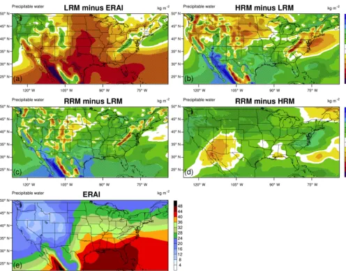
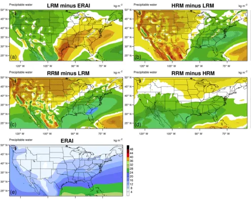
3.2.2 Precipitable water

Figures 6 and 7 show the seasonal mean TMQ in JJA and DJF compared with the ERAI reanalysis data. The LRM un-derestimates the JJA TMQ over most places (see Fig. 6a) ex-cept the northwest US and smaller areas of the eastern US and Mexico, where we observe significantly overestimated precipitation in Fig. 4a. As suggested by the improvement of precipitation with increasing resolution in Fig. 2, the LRM underestimation is generally improved in the HRM (Fig. 6b) and the RRM (Fig. 6c). The mean RRM–HRM differences (Fig. 6d) are mostly positive (<4 kg m−2). This is due to reduction in precipitation in RRM than in HRM outside of

CONUS, where the RRM resolution is coarser than that of the HRM.

In DJF, the LRM TMQ (Fig. 7a) resembles the patterns (overestimation over the western US and underestimation over the eastern US) of precipitation (Fig. 5a) against evalua-tion data. Such similarity implies that the precipitaevalua-tion biases in winter are directly related to flaws in precipitable water. The RRM and the HRM differ less (mostly statistically in-significant, see Fig. 7d) than their differences with the LRM (Fig. 7b, c).

3.2.3 Low-level circulation

(11)

con-Q. Tang et al.: Regionally refined test bed in E3SM atmosphere model version 1 2689

Figure 6.Same as Fig. 4, but for total precipitable water (TMQ, unit: kg m−2) in JJA.

nections between the Great Plains LLJ events and regional precipitation anomalies in summer, such as greater precipita-tion over the north central US and Great Plains and declining precipitation along the Gulf coast and east coast. Here, we examine the 850 hPa horizontal wind speed (Figs 8 and 9; the difference vectors are shown by colors (magnitudes) and magenta streamlines (directions)) as an example of the low-level circulation.

In summer, the LRM simulates stronger wind than the ERAI reanalysis over a large portion of CONUS but a weaker southerly LLJ in the central US (see Fig. 8a), which con-tributes to the low precipitation bias in the Great Plains and along the Gulf coast in Fig. 4a. Enhancing resolution signifi-cantly strengthens the LLJ (Fig. 8b, c), consistent with results presented by Berg et al. (2015) for reanalyses with a range of resolutions, and reduces the differences compared to the ERAI reanalysis, since simulations at finer horizontal reso-lution can resolve the LLJ-related temperature and pressure gradients better than ones at coarser resolution. By contrast,

the overestimation of zonal wind strength over the northeast-ern US becomes slightly worse with finer resolution. The RRM–HRM (Fig. 8d) difference (mostly within±0.8 m s−1) is generally smaller than that in other panels, especially for the LLJ region over the south central US.

(12)

3.2.4 Surface air temperature

Warm and dry model biases over the summertime central US have been studied for more than a decade (Klein et al., 2006) and are still deficient in the current generation of regional and global climate models (Cheruy et al., 2014; Mueller and Seneviratne, 2014; Lin et al., 2017; Ma et al., 2018; Mor-crette et al., 2018). Land (soil moisture)–atmosphere cou-pling plays a key role in causing warm and dry biases (Mo and Juang, 2003; Klein et al., 2006; Lin et al., 2017; Ma et al., 2018; Van Weverberg et al., 2018) and the related precip-itation biases.

Figure 10 shows the mean JJA patterns of differences in T2 m between the LRM and ERAI data and between three EAMv1 model pairs over CONUS. Over the central US, the LRM simulation exhibits statistically significant posi-tive temperature (up to 3 K) biases throughout the area (see Fig. 10a), corresponding to precipitation low bias (Fig. 4a) in this region. As implied by the Taylor diagram (Fig. 2),

(13)

Figure 8.Same as Fig. 4, but for 850 hPa wind speed (unit: m s−1) in JJA. The vectors are shown by colors (magnitudes) and magenta streamlines (directions). Grid boxes where surface pressure is less than 850 hPa are shaded in gray in the difference plots.

Figure 11 shows the T2 m results in DJF. The LRM (Fig. 11a) still suffers from warm bias over the central US, but it is less severe and much less widespread than in JJA. Over almost the entire eastern US, the LRM underesti-mates (by up to 4 K) T2 m. The HRM (Fig. 11b) and RRM (Fig. 11c) simulations appear better than the LRM over the Great Plains, the north central US, and the southeastern US. The RRM–HRM differences in Fig. 11d are again the small-est among all panels and statistically insignificant except for the southwestern US.

So far, we have demonstrated that the RRM capability re-produces the characteristics of hydrologic fields simulated in HRM. This proves that the RRM is a reliable test bed which can be used to effectively study and understand these model biases. Next, we will present further analysis of precipitation with RRM and compare it with HRM. Note that the hydro-logical cycle is a major focus of E3SM of which precipitation is the most important atmospheric variable.

3.3 Precipitation characteristics

3.3.1 Partitioning between large-scale vs. convective precipitation

(14)

par-2692 Q. Tang et al.: Regionally refined test bed in E3SM atmosphere model version 1

Figure 9.Same as Fig. 8, but for DJF. Note that the color scale is different from that in Fig. 8.

titioning between the large-scale and convective precipita-tion is an important evaluaprecipita-tion metric for climate models. Al-though they can be clearly defined in the model, the two pre-cipitation components are difficult to separate observation-ally in a manner comparable to the model. Thus, we only plot the model results for the ratio.

Figures 12 and 13 display the mean ratio of large-scale to total precipitation from EAMv1 models in JJA and DJF, respectively. As expected, convection is a more important source of precipitation in summer and at lower latitudes. The ratio of the large-scale precipitation increases with resolution in Figs. 12 and 13 because more precipitation can be resolved with finer-resolution grids and thus classified as large-scale precipitation. Similar convective precipitation changes with resolution are reported by Bacmeister et al. (2014) for CAM4 and CAM5. Consequently, compared to the LRM, large-scale precipitation in the HRM and RRM is more prevalent (espe-cially in the north) during the summer months (see Fig. 12b, c) and is even more dominant during the winter months (see

Fig. 13b, c). In both seasons, the RRM matches the HRM overall distributions of the precipitation partitioning includ-ing some regional details, for example, the contour lines along the Sierra Nevada in California in DJF.

3.3.2 Precipitation intensity distribution

(15)

overes-Q. Tang et al.: Regionally refined test bed in E3SM atmosphere model version 1 2693

Figure 10.Same as Fig. 4, but for 2 m air temperature (T2 m, unit: K) in JJA.

timating the frequency of light to moderate rain compared to the GPCP1DD data.

Figure 14 shows EAMv1 vs. GPCP1DD intensity func-tions over CONUS in JJA and DJF. Before aggregating the distribution, modeled precipitation rates are interpolated with the ESMF conservative regridding method to the same 1◦×1◦grids as GPCP1DD data. All datasets are averaged over daily intervals. The frequency is then counted in log bins of precipitation rates on each grid. In this way, the frequency functions from datasets at different spatial and temporal resolutions become comparable. It is evident in Fig. 14 that EAMv1 still simulates excessive light precipita-tion (<10 mm d−1) with all three configurations in both JJA and DJF. As implied by the mean behaviors in Figs. 12 and 13, convective precipitation accounts for a larger fraction of the total in JJA than in DJF across the whole spectrum (not shown in Fig. 14). Total precipitation from the RRM (blue dots) is closer to the HRM (red dots) than to the LRM (green dots) in most bins. These results suggest that we can use the

RRM as a test bed to address issues of intensity statistics over CONUS in the HR configurations of future EAM versions.

(16)

Figure 12.Mean ratio of large-scale to total precipitation in JJA for(a)LRM,(b)HRM, and(c)RRM.

(17)

Figure 14.Daily mean precipitation frequency (unit: dF /d log(P )) functions of total precipitation for the GPCP1DD observation (black), and model simulations: LRM (green), HRM (red), and RRM (blue) in(a)JJA and(b)DJF. Before deriving the distribution, precipitation rates (unit: mm d−1) are interpolated to 1◦×1◦grids and averaged over daily intervals.

For example, Bacmeister et al. (2014) used the diurnal cy-cle of precipitation to diagnose deficiencies in capturing the observed phase of MCSs over the central US in CAM5 with both LR and HR configurations.

Figure 15 illustrates the mean diurnal phase and magnitude patterns of maximum precipitation in JJA from the NEXRAD data and the EAMv1 simulations. The mean diurnal maxi-mum is determined from the first harmonic of the Fourier series constructed from the hourly precipitation time series in each grid box. The phase (local time) of the maximum is indicated by colors, while the magnitude the saturation of the color. The NEXRAD data (Fig. 15a) show the distinct nocturnal (19:00—04:00 LT, UTC−6 h) peak over the cen-tral US. This nocturnal peak has been attributed to the east-ward propagation of MCSs originating at the front range of Rocky Mountains in the afternoon (Riley et al., 1987; Dai et al., 1999; Carbone et al., 2002; Jiang et al., 2006; Dirmeyer et al., 2012). Unfortunately, no model configuration is suc-cessful at capturing this nighttime maximum. The RRM and HRM diurnal phases are similar and show modest improve-ment over the LRM in the sense that they have weaker am-plitudes (lighter colors in panels c and d than in panel b) of incorrect diurnal cycles. The similarity between RRM and HRM indicates that RRM simulations will be valuable for understanding and addressing this important model bias.

To evaluate the known eastward propagation feature of the convection in this area, we average the JJA precipita-tion over four subregions: mountains, high plains, middle plains, and low plains, outlined by solid square boxes on Fig. 15a. Figure 16 shows the mean composite diurnal cy-cle in these subregions. We first calculate the simple mean diurnal cycle from the hourly time series for each grid box. The first and second diurnal harmonics of the mean diurnal cycle – obtained using fast Fourier transform – are retained and adjusted to local time to generate the composite diurnal cycle. The composite lines plotted in Fig. 16 are averages

of the composite diurnal cycle in each grid box within the subregions. In the NEXRAD measurements (Fig. 16a), there is a clear propagating pattern: the maximum emerges over the mountains (black) in the afternoon at 15:00 LT, moves eastward and intensifies across the Great Plains, and reaches the middle (blue) and the low (green) plains in the night at 20:00 and 00:00 LT, respectively. The three EAMv1 simula-tions (Fig. 16b–d) do not reproduce the convection propa-gation and miss the nocturnal precipitation peak. Although the HRM and the RRM show better skill than the LRM from the mountains to the high plains, these convective events are not strong enough (smaller magnitudes compared to obser-vations) to sustain propagation further east.

(18)

Figure 15.Mean diurnal phase (local time; unit: hours) and magnitude (unit: mm d−1) of the maximum precipitation in JJA calculated from the first harmonic for(a)NEXRAD observations,(b)LRM,(c)HRM, and(d)RRM. The phase is indicated by colors, while the magnitude is indicated by the saturation of the color. In panel(a), the solid boxes denote four central US regions from west to east: mountains (37–40◦N, 105–108◦W), high plains (37–40◦N, 101–104◦W), middle plains (37–40◦N, 97–100◦W), and low plains (37–40◦N, 93–96◦W). The dashed box marks the southeast (31–34◦N, 82–90◦W) regions.

(19)

Q. Tang et al.: Regionally refined test bed in E3SM atmosphere model version 1 2697 to the HRM and report the results in a future paper. This bias

in the diurnal cycle of convection is significantly improved in convection-permitting (horizontal grid spacing<2–4 km) simulations (Prein et al., 2015). The E3SM project is mak-ing progress in developmak-ing its convection-permittmak-ing version (E3SMv4), for which the RRM test bed will be heavily relied on.

4 Nudging capability for RRM

Nudging is an effective technique to create quasi-deterministic model realizations of observations for a spe-cific time period. There is increasing use of nudging in cli-mate model development and evaluation of physical parame-terizations (e.g., Jeuken et al., 1996; Ghan et al., 2001; Koop-erman et al., 2012; Zhang et al., 2014). Since nudging simu-lations constrain the model states closer to observed meteoro-logical conditions, they facilitate the evaluation of modeled physics during specific meteorological episodes. Therefore, nudging can help advance process-level understanding of physical phenomena and ultimately improve physical param-eterizations. This is similar to the hindcast approach (Phillips et al., 2004; Ma et al., 2015) that has been widely used for cli-mate model evaluation. EAMv1 has a built-in nudging capa-bility as part of its physics module. When running the nudged RRM, one has various choices available such as nudging variables, locations, and timescales. In this section, we will provide an example of the value of EAMv1 RRM nudging simulations.

The EAMv1 nudging capability in the physics module al-lows the relaxation of model state variables (U,V,T, and specific humidity, or a subset thereof) towards analysis or re-analysis data. The nudging strength is determined by a frac-tional nudging coefficient between 0 and 1, which can be a spatial constant or a spatial variable specified by a Heaviside window function. Following previous findings by Zhang et al. (2014) and Ma et al. (2015), we opt to only nudge hori-zontal velocities for better cloud and aerosol properties with a 6 h relaxation timescale (see Eq. 1 of Zhang et al., 2014). The nudging coefficient map is shown in Fig. 17. The corre-sponding nudging parameter settings are documented in Ta-ble 3. This non-US nudging setting creates a smooth transi-tion from the strongest nudging (red) over coarser grid points to the weakest nudging (blue) over finer grid points. Running in this mode builds a pseudo-regional model framework in a global model. It gives the simulation more freedom over part of the HR region and reduces the nudging noise due to inconsistency between the model and analysis data over the free-running region for better evaluation of physics over this region.

As an example of the nudging results, we create the Hov-möller diagrams (Fig. 18) of hourly mean total precipita-tion, meridionally averaged over 35–45◦N, 93–115◦W (the magenta box in Fig. 17) during the period of the DOE

At-Figure 17.Nudging coefficient map zoom-in over North America. A coefficient of 0 indicates that no nudging is applied. The magenta box marks the area of the Hovmöller plots in Fig. 18.

Table 3.Nudging parameter settings for the non-US nudging simu-lation.

Nudging parameter Value

Nudge_Model .true.

Nudge_Path Path to analysis or reanalysis data

(20)

Figure 18.Hovmöller plots of hourly mean total precipitation (unit: mm d−1) over 35–45◦N, 93–115◦W during 22 April–6 June 2011 for

(a)NEXRAD observations,(b)AMIP LRM, and(c)nudging RRM.

mospheric Radiation Measurement (ARM) Facility’s Mid-latitude Continental Convective Clouds Experiment (MC3E, 22 April–6 June 2011) (Jensen et al., 2016). The main sci-ence goal of the MC3E campaign is to improve the under-standing of midlatitude continental convective cloud systems and their interactions with the environment (Xie et al., 2014). Many cloud and precipitation events are observed and clearly shown in the NEXRAD panel (Fig. 18a), such as convective events on 25 April and around 23 May and widespread strat-iform rain on 10 May. As expected, the AMIP simulation (Fig. 18b) struggles to capture the statistics of these high-frequency weather systems. The RRM nudging simulation (Fig. 18c) reproduces the timing and location of most events because nudging the horizontal velocities outside of the ana-lyzed area provides more realistic boundary conditions of the large-scale circulation in the free-running domain. There are still some deficiencies in the nudged simulation, for exam-ple the incorrect number and propagating speed of convec-tive events, particularly after 15 May. The nudged RRM has cleanly separated these remaining (model-deficiency-based) problems from issues related to the large-scale circulation. This demonstrates that the nudged RRM is an effective test bed for isolating and fixing parameterization problems at res-olutions we cannot afford to run globally.

5 Summary and discussion

We have presented an overview of the climatological results comparing initial atmosphere-only simulations from globally uniform low resolution (LR, 1◦), high resolution (HR, 0.25◦), and the regionally refined model (RRM, 1 to 0.25◦) over the contiguous US (CONUS) with the atmosphere model version 1 (EAMv1) using the Energy Exascale Earth

Sys-tem Model (E3SM). Our analysis has established that the RRM can generally mimic HR model (HRM) climate be-havior over the finely resolved portion (CONUS) for both well-simulated larger-scale thermodynamics fields and less satisfactory smaller-scale physical variables.

Similar to other models (Dai, 2006; Bacmeister et al., 2014), the EAMv1 HRM suffers from deficiencies in con-vection, clouds, and moist physics (Xie et al., 2018). To ver-ify that the RRM is a suitable alternative framework to the HRM to address these deficiencies, we examine the seasonal mean geographic patterns of precipitation, vertically inte-grated precipitable water, low-level circulation, and surface temperature for JJA and DJF. Given its key importance in the atmospheric hydrologic cycle, we conduct in-depth anal-ysis on precipitation, including fractions of the large-scale precipitation and daily intensity functions, and the JJA diur-nal cycle. Overall, the RRM is similar to the HRM for many finer-scale features, including reproducing long-standing cli-mate model biases, such as a lack of summertime nocturnal precipitation peaks and the warm bias in surface air temper-ature.

(21)

Q. Tang et al.: Regionally refined test bed in E3SM atmosphere model version 1 2699 how RRMs can be used as a useful test bed to evaluate

po-tentially improved schemes across different spatial scales. To help users better utilize the E3SM RRM capability, we provide detailed guidance on running the RRM in the nudg-ing mode so that deficiencies in model physical parameter-izations can be better isolated. By relaxing the horizontal velocities over coarser-resolution grids to analysis data, we create more realistic boundary conditions to the free-running higher-resolution area. Such a pseudo-regional model frame-work within a global model displays great advantages in cap-turing observed convective episodes over the AMIP config-uration and hence allows us to calibrate simulated physical processes against observations under different meteorolog-ical conditions. With more realistic large-scale circulation conditions, the nudged RRM can be used as a physics test bed for regional process-level studies and aid in the develop-ment of future HR EAM versions.

Code availability. The E3SM source code is available on GitHub: https://github.com/E3SM-Project/E3SM (last access: 2 July 2019; E3SM Project, DOE, 2018).

(22)

2700 Q. Tang et al.: Regionally refined test bed in E3SM atmosphere model version 1 Appendix A

Table A1.EAMv1 simulation setup details.

Simulation Code hash Grid Compset

Low-resolution model (LRM) 7a17edbe5 ne30_ne30 FC5AV1C-04P2

High-resolution model (HRM) 66793a1d3 ne120_ne120 FC5AV1C-H01A

Regionally refined model (RRM) 7a17edbe5 conusx4v1_conusx4v1 FC5AV1C-04P2∗

RRM_LR 7a17edbe5 conusx4v1_conusx4v1 FC5AV1C-04P2

LRM AMIP dd18fc56e ne30_oECv3 F20TRC5-CMIP6

RRM non-US nudging 7a17edbe5 conusx4v1_conusx4v1 FC5AV1C-04P2∗

∗_{Used non-default parameter values in Table A2.}

Table A2.Non-default parameter values.

Parameter Value

cldfrc_dp1 0.03

clubb_c14 1.75

clubb_c8 4.73

rsplit 2

se_nsplit 6

cld_macmic_num_steps 3

zmconv_alfa 0.2

zmconv_c0_lnd 0.0035

zmconv_c0_ocn 0.0043

zmconv_dmpdz −0.2×10−3

(23)

Q. Tang et al.: Regionally refined test bed in E3SM atmosphere model version 1 2701 Appendix B: Abbreviations list

ACME Accelerated Climate Modeling for Energy AMIP Atmospheric Model Intercomparison Project ARM Atmospheric Radiation Measurement

CALIPSO Cloud-Aerosol Lidar and Infrared Pathfinder Satellite Observation

CAM Community Atmosphere Model

CERES-EBAF Clouds and the Earth’s Radiant Energy System—Energy Balanced and Filled CESM Community Earth System Model

CLUBB Cloud Layers Unified By Binormals CONUS Contiguous United States

COSP Cloud Feedback Model Intercomparison Project Observation Simulator Package CSSEF Climate Science for a Sustainable Energy Future

DJF December–January–February

DOE Department of Energy

E3SM Energy Exascale Earth System Model

EAM E3SM atmosphere model

EF Evaporative fraction

ENA Eastern North Atlantic

ERAI European Centre for Medium-range Weather Forecasting Interim ESMF Earth System Modeling Framework

GPCP Global Precipitation Climatology Project GPCP1DD GPCP 1◦daily

HR High-resolution

HRM High-resolution model

ISCCP International Satellite Cloud Climatology Project

JJA June–July–August

KNL Knights Landing

Linoz Linearized ozone chemistry

LLJ Low-level jet

LR Low-resolution

LRM Low-resolution model

MAM Modal Aerosol Module

MCC Mesoscale Convective Complex

MC3E Midlatitude Continental Convective Clouds Experiment MCS Mesoscale convective system

MODIS Moderate Resolution Imaging Spectroradiometer NERSC National Energy Research Scientific Computing Center NEXRAD Next-Generation Radar

OMEGA500 500 hPa vertical velocity PRECT Total precipitation

rms Root-mean-square

RRM Regionally refined model

SD Standard deviation

SST Sea surface temperature TMQ Total precipitable water TREFHT Reference height temperature TWP Tropical western Pacific U200 200 hPa zonal wind

US United States

(24)

Author contributions. QT and SAK designed the experiments. QT and WL performed the simulations and analyzed the data. QT, SAK, and SX designed the scope and structure of the paper. QT prepared the paper with contributions from all coauthors.

Competing interests. The authors declare that they have no conflict of interest.

Acknowledgements. This research was primarily supported as part of the Energy Exascale Earth System Model (E3SM) project and partially supported by the Climate Model Development and Valida-tion activity, Atmospheric System Research Program, and an earlier project entitled Climate Science for a Sustainable Energy Future, funded by the U.S. Department of Energy (DOE), Office of Science, Office of Biological and Environmental Research (BER) under the auspices of the U.S. DOE by Lawrence Livermore National Labora-tory under contract DE-AC52-07NA27344. The Pacific Northwest National Laboratory is operated for DOE by the Battelle Memo-rial Institute under contract DE-A06-76RLO 1830. This paper has been authored by employees of Brookhaven Science Associates, LLC, under contract no. DE-SC0012704 with the U.S. DOE. The publisher by accepting the paper for publication acknowledges that the U.S. Government retains a nonexclusive, paid-up, irrevocable, world-wide license to publish or reproduce the published form of this paper, or allow others to do so, for U.S. Government pur-poses. This research used resources of the National Energy Re-search Scientific Computing Center, a DOE Office of Science User Facility supported by the Office of Science of the U.S. DOE un-der contract no. DE-AC02-05CH11231. The authors thank Christo-pher Terai for providing the GPCP1DD data. The authors also thank Jonathan J. Gourley and Zac Flamig of the National Severe Storms Laboratory for access to the archives of NEXRAD NMQ Q2/3 prod-ucts used in this study. The release number is LLNL-JRNL-764721.

Review statement. This paper was edited by Patrick Jöckel and re-viewed by two anonymous referees.

References

Ashley, W. S., Mote, T. L., Dixon, P. G., Trotter, S. L., Powell, E. J., Durkee, J. D., and Grundstein, A. J.: Distribution of Mesoscale Convective Complex Rainfall in the United States, Mon. Weather Rev., 131, 3003–3017, https://doi.org/10.1175/1520-0493(2003)131<3003:DOMCCR>2.0.CO;2, 2003.

Bacmeister, J. T., Wehner, M. F., Neale, R. B., Gettelman, A., Han-nay, C., Lauritzen, P. H., Caron, J. M., and Truesdale, J. E.: Ex-ploratory High-Resolution Climate Simulations using the Com-munity Atmosphere Model (CAM), J. Climate, 27, 3073–3099, https://doi.org/10.1175/JCLI-D-13-00387.1, 2014.

Bader, D. C., Collins, W., Jacob, R., Jones, P., Rasch, P., Taylor, M., Thornton, P., and Williams, D.: Accelerated Climate Modeling for Energy, available at: https://e3sm.org/wp-content/uploads/ 2018/03/ACME-project-strategy-July-2014.pdf (last access: 10 January 2019), 2014.

Bechtold, P., Chaboureau, J.-P., Beljaars, A., Betts, A. K., Köh-ler, M., MilKöh-ler, M., and Redelsperger, J.-L.: The simulation of the diurnal cycle of convective precipitation over land in a global model, Q. J. Roy. Meteor. Soc., 130, 3119–3137, https://doi.org/10.1256/qj.03.103, 2004.

Bechtold, P., Semane, N., Lopez, P., Chaboureau, J.-P., Beljaars, A., and Bormann, N.: Representing Equilibrium and Nonequilibrium Convection in Large-Scale Models, J. Atmos. Sci., 71, 734–753, https://doi.org/10.1175/JAS-D-13-0163.1, 2014.

Berg, L. K., Riihimaki, L. D., Qian, Y., Yan, H., and Huang, M.: The Low-Level Jet over the Southern Great Plains Determined from Observations and Reanalyses and Its Impact on Moisture Trans-port, J. Climate, 28, 6682–6706, https://doi.org/10.1175/JCLI-D-14-00719.1, 2015.

Bodas-Salcedo, A., Webb, M. J., Bony, S., Chepfer, H., Dufresne, J.-L., Klein, S. A., Zhang, Y., Marchand, R., Haynes, J. M., Pin-cus, R., and John, V. O.: COSP: Satellite simulation software for model assessment, B. Am. Meteorol. Soc., 92, 1023–1043, https://doi.org/10.1175/2011BAMS2856.1, 2011.

Bogenschutz, P. A., Gettelman, A., Morrison, H., Larson, V. E., Craig, C., and Schanen, D. P.: Higher-Order Turbu-lence Closure and Its Impact on Climate Simulations in the Community Atmosphere Model, J. Climate, 26, 9655–9676, https://doi.org/10.1175/JCLI-D-13-00075.1, 2013.

Carbone, R. E., Tuttle, J. D., Ahijevych, D. A., and

Trier, S. B.: Inferences of Predictability Associated

with Warm Season Precipitation Episodes, J.

At-mos. Sci., 59, 2033–2056, https://doi.org/10.1175/1520-0469(2002)059<2033:IOPAWW>2.0.CO;2, 2002.

Chepfer, H., Bony, S., Winker, D., Cesana, G., Dufresne, J. L., Min-nis, P., Stubenrauch, C. J., and Zeng, S.: The GCM-Oriented CALIPSO Cloud Product (CALIPSO-GOCCP), J. Geophys. Res., 115, D00H16, https://doi.org/10.1029/2009JD012251, 2010.

Cheruy, F., Dufresne, J. L., Hourdin, F., and Ducharne, A.: Role of clouds and land-atmosphere coupling in midlatitude conti-nental summer warm biases and climate change amplification in CMIP5 simulations, Geophys. Res. Lett., 41, 6493–6500, https://doi.org/10.1002/2014GL061145, 2014.

Dai, A.: Precipitation Characteristics in Eighteen

Cou-pled Climate Models, J. Climate, 19, 4605–4630,

https://doi.org/10.1175/JCLI3884.1, 2006.

Dai, A., Giorgi, F., and Trenberth, K. E.: Observed and model-simulated diurnal cycles of precipitation over the contigu-ous United States, J. Geophys. Res.-Atmos., 104, 6377–6402, https://doi.org/10.1029/98JD02720, 1999.

Dee, D. P., Uppala, S. M., Simmons, A. J., Berrisford, P., Poli, Kobayashi, S., Andrae, U., Balmaseda, M. A., Balsamo, G., Bauer, P., Bechtold, P., Beljaars, A. C. M., van de Berg, L., Bid-lot, J., Bormann, N., Delsol, C., Dragani, R., Fuentes, M., Geer, A. J., Haimberger, L., Healy, S. B., Hersbach, H., Hólm, E. V., Isaksen, L., Kållberg, P., Köhler, M., Matricardi, M., McNally, A. P., Monge-Sanz, B. M., Morcrette, J.-J., Park, B.-K., Peubey, C., de Rosnay, P., Tavolato, C., Thépaut, J.-N., and Vitart, F.: The ERA-Interim reanalysis: configuration and performance of the data assimilation system, Q. J. Roy. Meteor. Soc., 137, 553–597, https://doi.org/10.1002/qj.828, 2011.

(25)

CAM-Q. Tang et al.: Regionally refined test bed in E3SM atmosphere model version 1 2703

SE: A scalable spectral element dynamical core for the Com-munity Atmosphere Model, Int. J. High Perform. C., 26, 74–89, https://doi.org/10.1177/1094342011428142, 2012.

Dirmeyer, P. A., Cash, B. A., Kinter, J. L., Jung, T., Marx, L., Satoh, M., Stan, C., Tomita, H., Towers, P., Wedi, N., Achuthavarier, D., Adams, J. M., Altshuler, E. L., Huang, B., Jin, E. K., and Man-ganello, J.: Simulating the diurnal cycle of rainfall in global cli-mate models: resolution versus parameterization, Clim. Dynam., 39, 399–418, https://doi.org/10.1007/s00382-011-1127-9, 2012. E3SM Project, DOE: Energy Exascale Earth System Model, Com-puter Software, https://doi.org/10.11578/E3SM/dc.20180418.36, 2018.

Fournier, A., Taylor, M. A., and Tribbia, J. J.: The Spectral El-ement Atmosphere Model (SEAM): High-Resolution Parallel Computation and Localized Resolution of Regional Dynamics, Mon. Weather Rev., 132, 726–748, https://doi.org/10.1175/1520-0493(2004)132<0726:TSEAMS>2.0.CO;2, 2004.

Gettelman, A. and Morrison, H.: Advanced Two-Moment Bulk Microphysics for Global Models. Part I: Off-Line Tests and Comparison with Other Schemes, J. Climate, 28, 1268–1287, https://doi.org/10.1175/JCLI-D-14-00102.1, 2015.

Gettelman, A., Callaghan, P., Larson, V. E., Zarzycki, C. M., Bacmeister, J. T., Lauritzen, P. H., Bogenschutz, P. A., and Neale, R. B.: Regional Climate Simulations With the Community Earth System Model, J. Adv. Model. Earth Syst., 10, 1245–1265, https://doi.org/10.1002/2017MS001227, 2018.

Ghan, S., Laulainen, N., Easter, R., Wagener, R., Nemesure, S., Chapman, E., Zhang, Y.. and Leung, R.: Evaluation of aerosol direct radiative forcing in MIRAGE, J. Geophys. Res.-Atmos., 106, 5295–5316, https://doi.org/10.1029/2000JD900502, 2001. Giangrande, S. E., Collis, S., Theisen, A. K., and Tokay, A.:

Pre-cipitation Estimation from the ARM Distributed Radar Network during the MC3E Campaign, J. Appl. Meteorol. Clim., 53, 2130– 2147, https://doi.org/10.1175/JAMC-D-13-0321.1, 2014. Gleckler, P., Doutriaux, C., Durack, P., Taylor, K. E., Zhang, Y.,

Williams, D., Mason, E., and Servonnat, J.: A more powerful reality test for climate models, Eos Trans. Am. Geophys. Union, 97, https://doi.org/10.1029/2016EO051663, 2016.

Golaz, J.-C., Larson, V. E., and Cotton, W. R.: A

PDF-Based Model for Boundary Layer Clouds.

Part I: Method and Model Description, J. Atmos.

Sci., 59, 3540–3551,

https://doi.org/10.1175/1520-0469(2002)059<3540:APBMFB>2.0.CO;2, 2002.

Golaz, J.-C., Caldwell, P. M., Van Roekel, L. P., Petersen, M. R., Tang, Q., Wolfe, J. D., Abeshu, G., Anantharaj, V., Asay-Davis, X. S., Bader, D. C., Baldwin, S. A., Bisht, G., Bogenschutz, P. A., Branstetter, M., Brunke, M. A., Brus, S. R., Burrows, S. M., Cameron-Smith, P. J., Donahue, A. S., Deakin, M., Easter, R. C., Evans, K. J., Feng, Y., Flanner, M., Foucar, J. G., Fyke, J. G., Griffin, B. M., Hannay, C., Harrop, B. E., Hunke, E. C., Ja-cob, R. L., Jacobsen, D. W., Jeffery, N., Jones, P. W., Keen, N. D., Klein, S. A., Larson, V. E., Leung, L. R., Li, H.-Y., Lin, W., Lipscomb, W. H., Ma, P.-L., Mahajan, S., Maltrud, M. E., Mametjanov, A., McClean, J. L., McCoy, R. B., Neale, R. B., Price, S. F., Qian, Y., Rasch, P. J., Reeves Eyre, J. E. J., Riley, W. J., Ringler, T. D., Roberts, A. F., Roesler, E. L., Salinger, A. G., Shaheen, Z., Shi, X., Singh, B., Tang, J., Taylor, M. A., Thornton, P. E., Turner, A. K., Veneziani, M., Wan, H., Wang, H., Wang, S., Williams, D. N., Wolfram, P. J., Worley, P. H., Xie,

S., Yang, Y., Yoon, J.-H., Zelinka, M. D., Zender, C. S., Zeng, X., Zhang, C., Zhang, K., Zhang, Y., Zheng, X., Zhou, T., and Zhu, Q.: The DOE E3SM coupled model version 1: Overview and evaluation at standard resolution, J. Adv. Model. Earth Syst., 11, https://doi.org/10.1029/2018MS001603, accepted, 2019. Guba, O., Taylor, M. A., Ullrich, P. A., Overfelt, J. R., and

Levy, M. N.: The spectral element method (SEM) on variable-resolution grids: evaluating grid sensitivity and variable- resolution-aware numerical viscosity, Geosci. Model Dev., 7, 2803–2816, https://doi.org/10.5194/gmd-7-2803-2014, 2014.

Helfand, H. M. and Schubert, S. D.: Climatology of the Simulated Great Plains Low-Level Jet and Its Contribu-tion to the Continental Moisture Budget of the United States, J. Climate, 8, 784–806, https://doi.org/10.1175/1520-0442(1995)008<0784:COTSGP>2.0.CO;2, 1995.

Higgins, R. W., Yao, Y., Yarosh, E. S., Janowiak, J. E., and Mo, K. C.: Influence of the Great Plains Low-Level Jet on Summertime Precipitation and Moisture Transport over the Central United States, J. Climate, 10, 481–507, https://doi.org/10.1175/1520-0442(1997)010<0481:IOTGPL>2.0.CO;2, 1997.

Hsu, J. and Prather, M. J.: Stratospheric variability and tro-pospheric ozone, J. Geophys. Res.-Atmos., 114, D06102, https://doi.org/10.1029/2008JD010942, 2009.

Huang, X. and Ullrich, P. A.: The Changing Character of Twenty-First-Century Precipitation over the Western United States in the Variable-Resolution CESM, J. Climate, 30, 7555–7575, https://doi.org/10.1175/JCLI-D-16-0673.1, 2017.

Huffman, G. J., Adler, R. F., Morrissey, M. M., Bolvin,

D. T., Curtis, S., Joyce, R., McGavock, B., and

Susskind, J.: Global Precipitation at One-Degree Daily Resolution from Multisatellite Observations, J. Hy-drometeorol., 2, 36–50, https://doi.org/10.1175/1525-7541(2001)002<0036:GPAODD>2.0.CO;2, 2001.

Huffman, G. J., Adler, R. F., Bolvin, D. T., and Gu, G.: Improving the global precipitation record: GPCP Version 2.1, Geophys. Res. Lett., 36, L17808, https://doi.org/10.1029/2009GL040000, 2009. IPCC: Managing the Risks of Extreme Events and Disasters to Ad-vance Climate Change Adaptation, A Special Report of Work-ing Groups I and II of the Intergovernmental Panel on Climate Change, edited by: Field, C. B., Barros, V., Stocker, T. F., Qin, D., Dokken, D. J., Ebi, K. L., Mastrandrea, M. D., Mach, K. J., Plattner, G.-K., Allen, S. K., Tignor, M., and Midgley, P. M., Cambridge University Press, Cambridge, UK, and New York, NY, USA, 2012.

Jensen, M. P., Petersen, W. A., Bansemer, A., Bharadwaj, N., Carey, L. D., Cecil, D. J., Collis, S. M., Del Genio, A. D., Dolan, B., Gerlach, J., Giangrande, S. E., Heymsfield, A., Heymsfield, G., Kollias, P., Lang, T. J., Nesbitt, S. W., Neumann, A., Poellot, M., Rutledge, S. A., Schwaller, M., Tokay, A., Williams, C. R., Wolff, D. B., Xie, S., and Zipser, E. J.: The Midlatitude Conti-nental Convective Clouds Experiment (MC3E), B. Am. Meteo-rol. Soc., 97, 1667–1686, https://doi.org/10.1175/BAMS-D-14-00228.1, 2016.

(26)

Jiang, X., Lau, N., and Klein, S. A.: Role of eastward propagating convection systems in the diurnal cycle and seasonal mean of summertime rainfall over the U.S. Great Plains, Geophys. Res. Lett., 33, L19809, https://doi.org/10.1029/2006GL027022, 2006. Klein, S. A., Jiang, X., Boyle, J., Malyshev, S., and Xie, S.: Di-agnosis of the summertime warm and dry bias over the U.S. Southern Great Plains in the GFDL climate model using a weather forecasting approach, Geophys. Res. Lett., 33, L18805, https://doi.org/10.1029/2006GL027567, 2006.

Klein, S. A., Zhang, Y., Zelinka, M. D., Pincus, R., Boyle, J., and Gleckler, P. J.: Are climate model simulations of clouds improv-ing? An evaluation using the ISCCP simulator, J. Geophys. Res.-Atmos., 118, 1329–1342, https://doi.org/10.1002/jgrd.50141, 2013.

Kooperman, G. J., Pritchard, M. S., Ghan, S. J., Wang, M., Somerville, R. C. J., and Russell, L. M.: Constraining the in-fluence of natural variability to improve estimates of global aerosol indirect effects in a nudged version of the Community Atmosphere Model 5, J. Geophys. Res.-Atmos., 117, D23204, https://doi.org/10.1029/2012JD018588, 2012.

Lin, Y., Zhao, M., Ming, Y., Golaz, J.-C., Donner, L. J., Klein, S. A., Ramaswamy, V., and Xie, S.: Precipitation Partitioning, Tropical Clouds, and Intraseasonal Variability in GFDL AM2, J. Climate, 26, 5453–5466, https://doi.org/10.1175/JCLI-D-12-00442.1, 2013.

Lin, Y., Dong, W., Zhang, M., Xie, Y., Xue, W., Huang, J., and Luo, Y.: Causes of model dry and warm bias over central U.S. and impact on climate projections, Nat. Commun., 8, 881, https://doi.org/10.1038/s41467-017-01040-2, 2017.

Liu, X., Ma, P.-L., Wang, H., Tilmes, S., Singh, B., Easter, R. C., Ghan, S. J., and Rasch, P. J.: Description and evaluation of a new four-mode version of the Modal Aerosol Module (MAM4) within version 5.3 of the Community Atmosphere Model, Geosci. Model Dev., 9, 505–522, https://doi.org/10.5194/gmd-9-505-2016, 2016.

Loeb, N. G., Lyman, J. M., Johnson, G. C., Allan, R. P., Doelling, D. R., Wong, T., Soden, B. J., and Stephens, G. L.: Observed changes in top-of-the-atmosphere radiation and upper-ocean heating consistent within uncertainty, Nat. Geosci., 5, 110–113, https://doi.org/10.1038/ngeo1375, 2012.

Ma, H.-Y., Xie, S., Klein, S. A., Williams, K. D., Boyle, J. S., Bony, S., Douville, H., Fermepin, S., Medeiros, B., Tyteca, S., Watan-abe, M., and Williamson, D.: On the Correspondence between Mean Forecast Errors and Climate Errors in CMIP5 Models, J. Climate, 27, 1781–1798, https://doi.org/10.1175/JCLI-D-13-00474.1, 2014.

Ma, H.-Y., Chuang, C. C., Klein, S. A., Lo, M.-H., Zhang, Y., Xie, S., Zheng, X., Ma, P.-L., Zhang, Y., and Phillips, T. J.: An im-proved hindcast approach for evaluation and diagnosis of phys-ical processes in global climate models, J. Adv. Model. Earth Syst., 7, 1810–1827, https://doi.org/10.1002/2015MS000490, 2015.

Ma, H.-Y., Klein, S. A., Xie, S., Zhang, C., Tang, S., Tang, Q., Morcrette, C. J., Van Weverberg, K., Petch, J., Ahlgrimm, M., Berg, L. K., Cheruy, F., Cole, J., Forbes, R., Gustafson, W. I., Huang, M., Liu, Y., Merryfield, W., Qian, Y., Roehrig, R., and Wang, Y.-C.: CAUSES: On the Role of Surface Energy Budget Errors to the Warm Surface Air Temperature Error Over the

Cen-tral United States, J. Geophys. Res.-Atmos., 123, 2888–2909, https://doi.org/10.1002/2017JD027194, 2018.

Maddox, R. A.: Meoscale Convective Complexes, B. Am. Meteorol. Soc., 61, 1374–1387, https://doi.org/10.1175/1520-0477(1980)061<1374:MCC>2.0.CO;2, 1980.

Mo, K. C. and Juang, H. H.: Relationships between soil moisture and summer precipitation over the Great Plains and the Southwest, J. Geophys. Res.-Atmos., 108, 8610, https://doi.org/10.1029/2002JD002952, 2003.

Morcrette, C. J., Van Weverberg, K., Ma, H.-Y., Ahlgrimm, M., Bazile, E., Berg, L. K., Cheng, A., Cheruy, F., Cole, J., Forbes, R., Gustafson, W. I., Huang, M., Lee, W.-S., Liu, Y., Mellul, L., Merryfield, W. J., Qian, Y., Roehrig, R., Wang, Y.-C., Xie, S., Xu, K.-M., Zhang, C., Klein, S., and Petch, J.: Introduction to CAUSES: Description of Weather and Climate Models and Their Near-Surface Temperature Errors in 5 day Hindcasts Near the Southern Great Plains, J. Geophys. Res.-Atmos., 123, 2655– 2683, https://doi.org/10.1002/2017JD027199, 2018.

Mueller, B. and Seneviratne, S. I.: Systematic land climate and evapotranspiration biases in CMIP5 simulations, Geophys. Res. Lett., 41, 128–134, https://doi.org/10.1002/2013GL058055, 2014.

Neale, R. B., Chen, C. C., Gettelman, A., Lauritzen, P. H., Park, S., Williamson, D. L., Conley, A. J., Garcia, R., Kin-nison, D., Lamarque, J. F., Marsh, D., Mills, M., Smith, A. K., Tilmes, S., Vitt, F., Cameron-Smith, P., Collins, W. D., Ia-cono, M. J., Easter, R. C., Ghan, S. J., Liu, X., Rasch, P. J., and Taylor, M. A.: Description of the NCAR Community At-mosphere Model (CAM5.0), Tech. Note NCAR/TN-486+STR, 274 pp., available at: http://www.cesm.ucar.edu/models/cesm1.0/ cam/docs/description/cam5_desc.pdf (last access: 2 July 2019), 2012.

NOAA: NOAA National Weather Service (NWS) Radar Operations Center (1991): NOAA Next Generation Radar (NEXRAD) Level 2 Base Data. NOAA National Centers for Environmental Infor-mation, https://doi.org/10.7289/V5W9574V, 2013.

Pendergrass, A. G. and Hartmann, D. L.: Changes in the Distribution of Rain Frequency and Intensity in Re-sponse to Global Warming, J. Climate, 27, 8372–8383, https://doi.org/10.1175/JCLI-D-14-00183.1, 2014.

Phillips, T. J., Potter, G. L., Williamson, D. L., Cederwall, R. T., Boyle, J. S., Fiorino, M., Hnilo, J. J., Olson, J. G., Xie, S., and Yio, J. J.: Evaluating Parameterizations in General Circulation Models: Climate Simulation Meets Weather Prediction, B. Am. Meteorol. Soc., 85, 1903–1915, https://doi.org/10.1175/BAMS-85-12-1903, 2004.

Pincus, R., Platnick, S., Ackerman, S. A., Hemler, R. S., and Patrick Hofmann, R. J.: Reconciling Simulated and Observed Views of Clouds: MODIS, ISCCP, and the Limits of Instrument Simula-tors, J. Climate, 25, 4699–4720, https://doi.org/10.1175/JCLI-D-11-00267.1, 2012.

Prein, A. F., Langhans, W., Fosser, G., Ferrone, A., Ban, N., Go-ergen, K., Keller, M., Tölle, M., Gutjahr, O., Feser, F., Brisson, E., Kollet, S., Schmidli, J., van Lipzig, N. P. M., and Leung, R.: A review on regional convection-permitting climate modeling: Demonstrations, prospects, and challenges, Rev. Geophys., 53, 323–361, https://doi.org/10.1002/2014RG000475, 2015. Pu, B. and Dickinson, R. E.: Diurnal Spatial Variability of