journal homepage: http://civiljournal.semnan.ac.ir/
Multi-Damage Detection for Steel Beam Structure
Reza Farokhzad1, Gholamreza Ghodrati Amiri2, Benyamin Mohebi3* and Mohsen Ghafory-Ashtiany4
1. Department of Civil Engineering, Science and Research Branch, Islamic Azad University, Tehran, Iran. 2. Professor, Center of Excellent for Fundamental Studies in Structural Engineering, School of Civil Engineering Iran University of Science and Technology, Tehran, Iran.
3. Assistant Professor, Faculty of Engineering, Imam Khomeini International University, Qazvin, Iran.
4. Professor, Structural Department, International Institute of Earthquake Engineering and Seismology, Tehran, Iran.
Corresponding author:[email protected]
ARTICLE INFO ABSTRACT
Article history:
Received: 20 December 2016 Accepted: 31 January 2017
Damage detection has been focused by researchers because of its importance in engineering practices. Therefore, different approaches have been presented to detect damage location in structures. However, the higher the accuracy of methods is required the more complex deliberations. Based on the conventional studies, it was observed that the damage locations and its size are associated with dynamic parameters of the structures. The main objective of this research is to present a sophisticated approach to detect the damage location using multi-objective genetic algorithm (MOGA) along with modified multi-objective genetic algorithm (MMOGA). In this approach natural frequencies are considered as the main dynamic parameters to detect the damage. The finite element method (FEM) is utilized to validate the accuracy of the results extracted from the natural frequencies analysis with consideration of the beams with different support conditions. Accordingly the results emphasize the high accuracy of the proposed method with the maximum error of 5%.
Keywords: Damage Detection Exact Method, Cantilever Beam,
Multi-objective genetic algorithm (MOGA),
Modified multi-objective genetic algorithm (MMOGA).
1. Introduction
Damage of structures may occur at the beginning of construction or during utilization for different reasons. In the latter, the damage might happen due to using improper material, lack of monitoring or
utilization of structures. Accordingly, the researchers have presented different methods for solving the mentioned important problem. All these methods are based on determining the specifications of structures using static and dynamic responses. The methods based on the static response determine the changing of deformations, stiffness, and sections' capacities through calculating strain and displacement of structures under certain static loads. Dynamic methods might be based on the modal and signal processing information. The ideas using modal information may formed through natural frequency, modal shapes, modal shape curvature, modal strain energy, elasticity, residual force curve, modified matrix and frequency response function. However, the methods using only natural frequencies of several first modes for identifying the exact location of damage have been less assessed. Natural frequencies of the first three modes are the simplest measurable dynamic parameters in the structures. Accordingly, they can be easily calculated through experimental methods such as modal hammer [1], determining ultrasonic wave [2], and other similar procedures.
Amezquita et al. [3]examine and compare the sensitivity of the Wavelet transform coefficients using various wavelets to detect crack in a model beam. Wavelet transform is a relatively new signal processing method which provides a time–frequency representation of the signal through time and scale window functions. Zhao et al. [4]applied a counter-propagation neural network to locate damage in beams.
In 2013, Goldfeld et al. [5] focused on the identification of damage using the alteration of modal frequencies in the beams. In this
research the stiffness distributed in the beam and the changes of modal frequencies happened in any modal shape have been considered to investigate the distribution, intensity and location of damage. They studied another concrete beam for assessing cracks and exact location of the beam crack. Perera et al. [6] investigated different damages in a beam and updated the damage through dynamic and static measurements. In 2013, Mehrjoo et al. [7] studied genetic algorithm and its application in identifying the damage of beam shape elements (Bernoulli beam elements). In this research the crack has been considered using torsional spring in the two dimensional 4- node elements. Then the exact location of crack has been identified using natural frequency. Finally, genetic algorithm has been used better solving the problem and increasing the speed of meeting final response. In 2011, Moradi et al. [8] used bees' algorithm for identifying the cracks in the beam shape structures. In order to conduct experimental investigation, several cracks have been created in the beams with the dimensions of 14×14mm in 400mm length in different distances and depts. The frequencies of the mentioned structure have been calculated in the first three modes. Then the approximately identified damage, presented in the tables, has been assessed and discussed in the laboratory status as well as using optimization algorithms. The different approach, based on modal parameter input, is described by Zang.[9] They reduced the size of the frequency response function (FRF) data by performing a modal analysis first. A radial basis function (RBF) network was successful in detecting errors in a cantilevered beam.
damage applying composed genetic algorithm and structural modal specifications. In all cases the numerical and experimental statuses have been considered for damaged and undamaged structures to investigate the effects of noises and calculation errors. Ghasemi et al. [11]introduced a critical excitation model and damage index for the M.O.D.F structure. Farokhzad et al [12] focused on the identification of damage based on Optimization via Simulation (OVS). This method is established based on the first three natural frequencies of the deep or semi-deep beams.
In this regard, for generalizing the obtained results, the beam shape structure was modeled in simply-supported, cantilever, clamped–clamped, simple–clamped beam support conditions. Then, the exact location and depth of damage is identified applying optimization algorithms of MOGA and MMOGA. The obtained results are expanded to 9, 5, and 3 lengths to height ratios of beam. The process of modeling and meeting final responses are presented in the following. In this research, the determination of damage intensity and its exact location is studied using dynamic responses of the first three natural frequencies of damaged deep beam.
2. Presenting the optimization
algorithms
The optimization methods based on the target response are a set of conditions and constraints through which the problem approaches towards optimum response after
trial and error efforts. Today, multi objective algorithms are frequently used for solving the problems with many alternatives. Multi objective genetic algorithm (MOGA)[12] and modified multi objective genetic algorithm are of the methods which make possible the meeting of optimum response considering the kind of input including rate and exact location of damage.[12]
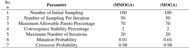
Table 1. Determining the different modeling parameters in MMOGA and MOGA
(MOGA) (MMOGA)
Parameter Ro
w
100 100
Number of Initial Sampling 1
50 50
Number of Sampling Per Iteration 2
70 70
Maximum Allowable Pareto Percentage 3
2 2
Convergence Stability Percentage 4
20 20
Maximum Number of Iterations 5
0.01 0.01
Mutation Probability 6
0.98 0.98
Crossover Probability 7
The MMOGA algorithm is very similar to genetic algorithm concerning its application excluding the generation and distribution of data. The distribution of data significantly affects the optimum response. Today, different methods are used in the world for creating primary population such as Mont Carlo [14, 15], Latin Hypercube Sampling [16] and filling space model [17], each with certain performances in the engineering. MMOGA [12] is mainly different from others in generating and distributing the data. In generation of data is random in the genetic algorithm while it is based on the Kriging algorithm in MMOGA. This algorithm can improve the optimum responses and adjust the output in accordance with the higher alternatives and create the Pareto level with reducing the errors. Actually, Kriging algorithm is an exact multi- dimensional insight, modeled by the simple polynomial function. Kriging algorithm has the capability of updating the error level in the recursive processes using Eq. (2-1). The error level is reduced in each repetition up to approaching of optimization process towards final response. In order to calculate the predicted relative error for a parameter, the error value obtained in each step is normalized to that of previous phase as follows:
normalized predicted error =relative predicted error Omax−Omin × 100 Eq. (2-1)
Where, Omin and Omax are maximum and minimum error values calculated for a parameter in a process, respectively. As mentioned earlier, this algorithm is formed by composing a multinomial simple model:
Y(x) = f(x) + Z(x) Eq. (2-2) Where, Y(x) is the values of location and
depth of damage; f(x) is the first three natural frequencies; Z(x) is a Gaussian process based on normal distribution with the mean of zero, σ2 variance and co-variance
of non-zero. In the other words, Z(x) is the value of error obtained according to Eq. (2-2) and the number of data (N). The value of co-variance Z(x) is calculated in the algorithm as follows:
COV[Z(xi), Z(xj)] = σ2R(r(xi, xj)) ) Eq. (2-3)
Where, R is the correlation matrix, a positive matrix with the diameter of N×N; r(xi, xj) is the spatial relation between two samples of N in the xj and xi points. The dependency of
r(xi, xj) is obtained based on the Gaussian
function as follows:
r(xi, xj) = exp [− ∑ θ
K|xki − xk j
|2 M
k=1 ] Eq. (2-4) θK Is an uncertain parameter used for fitting the model; M is the number of designing variables, here considered as 2 (the depth and distance of damage, xki and xkj are the kth component of the sample points of xj and xi.
which the optimum response is calculated. Maximum Allowable Pareto Percentage is the acceptance criterion indicating the ratio of the numbers of damaged points to the samples of each repetition. As this acceptance criterion reaches the allowable percentage, the optimization is convergent and the analysis is stopped. Convergence Stability Percentage is another acceptance criterion showing the optimization of population generated in each generation. It is calculated based on the mean deviation and standard. As the response obtained from optimization process is the same as the previous response, the analysis is convergent and is stopped. Mean deviation and standard deviation of the alternatives are controlled according to Eqs. (2-5, 2-6) and considering the generated population. If this value is equal to the previous one, the convergence has happened. The optimization is continued up to satisfying these relations.
|Meanj−Meanj−1| Max−Min <
S
100 Eq. (2-5)
|StdDevj−StdDevj−1|
Max−Min <
S
100 Eq. (2-6)
Where, S is Stability Percentage, here considered as 5; Meani is the mean of population in the Mth step; StdDevi is standard deviation criterion in the Mth step;
Max is maximum output calculated in the first generated data; Min is minimum output calculated in the first generated data. Stability percentage has been presented by abbreviation S in Eqs. (2-5, 2-6). As the S value is reduced, the accuracy of analysis increases, the convergence of analysis decreases and the optimization duration increases severely. In the other words, if S value is 5%, the difference between one generation and its previous corresponding one should be lower than 5%. This much indicates the high accuracies of results and convergence. Figure 1 presents a sample of Convergence Criteria Charts for clamped- clamped beam in three statuses.
Fig 1. Trial and error process in MMOGA algorithm for clamped- clamped beam
3. Calculating natural frequencies in
damage
and
undamaged
Timoshenko beam
Verification is the most important factor for insurance the optimization results. Exact methods are used to verify the obtained results through numerical methods. Dynamic specifications such as modal shape and modal frequency of a deep beam are calculated in damaged and undamaged
statuses, considering the formation of mass matrix and displacement vectors. The verification methods are assessed in the following.
3-1. Timoshenko undamaged beam
status based on the Eqs. (3-1, 3-2). The strain energy relation is calculated through Eq. (9) based on the reference [19].
k`G [∂2y(x,t) ∂x2 −
∂ψ(x,t) ∂x ] − ρ
∂2y(x,t)
∂t2 Eq. (3-1)
EI∂2∂xψ(x,t)2 + k`GA [∂y(x,t)
∂x − ψ(x, t)] − ρI ∂2y(x,t)
∂t2 = 0 Eq. (3-2)
U =1 2EI ∫ (
dϕ dx)
2 dx +1
2kAG ∫ ( ldψ
dx − ϕ) 2
dx Eq. (3-3)
In Eqs. (3-1, 3-2), G is shear modulus of material; k is shear coefficient of deep beam with Timoshenko behavior; E is elastic modulus of material; I:inertial moment of deep beam; A is the sectional area of beam; T is time; and ρ is specific gravity; ψ is general deformation. In Eq. (3-3), ψ̇ is general slope;
ϕ is the slope of curvature; ϕ́ is the first derivative of curvature slope; L: is the length
of assumed elements (two- node elements with 4 degrees of freedom); k is shear coefficient related to the beam surface with the values of6
5 for rectangular and 10
9 for
cyclic and 1 for I shape sections.
Based on Ref. [20], each ψ and ϕ functions and their derivatives are written in the forms of node displacements to obtain the general Eq. (3-4). The relation will become more complete by putting each supporting conditions.
{ξ}T=
[ ψi ϕi ψ́i ϕ́i ψi+1 ϕi+1 ψ́i+1 ϕi+1́ ]
[[K] − ωi2[M]]{ξi} = {0} Eq. (3-4)
In order to calculate the matrices of mass and stiffness in a deep beam with Timoshenko behavior using the Eqs.((3-1)-(3-4)) and based on the Ref. [20] to obtain matrices 3-5 and 3-6:
[K]=420lEI
[
504s 210s 42s 42s −504s 210s 42s −42s
210s 156s + 504 −42s 22s + 42 −210s 54s − 504 42s −13s + 42
42s −42s 56s 0 −42s 42s −14s −7s
42s 22s + 42 0 4s + 56 −42s 13s − 42 7s −3s − 14 −504s −210s −42s −42s 504s −210s −42s 42s
210s 54s − 504 42s 13s − 42 −210s 156s + 504 −42s −22s − 42
42s 42s −14s 7s −42s −42s 54s 0
−42s −13s + 42 −7s −3s − 14 42s −22s − 42 0 4s + 56 ]
Eq. (3-5)
In above matrix, s is shear matrix defined as:
s =KAGl2
EI Eq. (3-6)
[M] =ρAl3 420
[
156 0 22 0 54 0 −13 0
0 156R 0 22R 0 54R 0 −13R
22 0 4 0 13 0 −3 0
0 22R 0 4R 0 13R 0 −3R
54 0 13 0 156 0 −22 0
0 54R 0 13R 0 156R 0 −22R
−13 0 −3 0 −22 0 4 0
0 −13R 0 −3R 0 −22R 0 4R ]
Eq. (3-7)
Where R is inertial moment parameter, defined as follows
R= I
Al2 Eq. (3-8) Natural frequency of Timoshenko beam in the undamaged can be obtained by putting the above relations and placing the supporting conditions.
3-2. Timoshenko damaged beam
with exact solution method
through exact solving method based on the references [7, 21, 22]. Regarding Ref. [21], Khaji et al. presented mathematical solution for identifying the location of damage in the
deep beam with simply-supported, cantilever, clamped–clamped, simple–clamped supporting conditions.
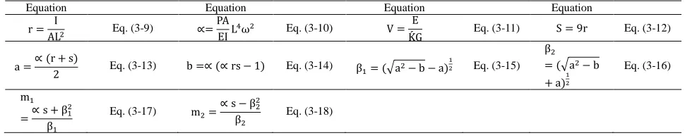
Table 2. Formulations coefficients based on Khaji et al.
Equation Equation Equation Equation
r = I
AL2 Eq. (3-9) ∝=
PA EIL
4ω2 Eq. (3-10) V = E
ḰG Eq. (3-11) S = 9r Eq. (3-12)
a =∝ (r + s)
2 Eq. (3-13) b =∝ (∝ rs − 1) Eq. (3-14) β1= (√a2− b − a)
1
2 Eq. (3-15) β2
= (√a2− b
+ a)12
Eq. (3-16)
m1
=∝ s + β1
2
β1
Eq. (3-17) m2=
∝ s − β22
β2
Eq. (3-18)
Natural frequencies of deep beams are obtained for a sample of simply- supported damaged beam as follows which can be taken from Ref. [17].
FSS(m1, m2, β1, β2, l1, l2)θ + GSS(m1, m2, β1, β2) = 0
Eq. (3-19) Where it can be written:
FSS(m1, m2, β1, β2, l1, l2) = m1β1(m2
+ β2) sin β2sinh l1β1sinh l2β1 + +m2β2(m1
− β1) sinh β1sin l1β2sin l2β2
GSS(m1, m2, β1, β2) = (m2β1+ m1β2) sin β2sinh β1
Eq. (3-20)
4. Modeling for verification of the
results of finite element and exact
solution method
In order to assess the considered method, a deep beam of building steel has been used
with the specific gravity of 7860 kg/m3, elasticity modulus of 210 (GPa) and poison ration of 0.3. The samples have cross section of 12.5×25 mm2 and the lengths of 225, 125 and 75 mm with the ratios of l/d=9, 5 and 3, respectively.
The real values of natural frequencies are calculated for the beam in damaged and undamaged statuses using the relations presented in section 3. The obtained first four natural frequencies have been represented in Tables 3, 4 and 5. The error (E %) and mean error (ME %) parameters are applied for comparing the numerical and exact solving methods. Mean error (ME %) is obtained from dividing total error values from natural frequencies of a beam by its numbers as per percentage.
The mentioned parameters have been investigated in different supporting statuses.
Table 3 presents briefly the calculations of the ratio to length to the height of l/d=9 for four supporting statuses. The distance and depth of damage have been considered as 112.5 mm and 12.5 mm, respectively, for its structural damage in the middle of beam. The maximum error values for E% and ME% parameters are 13.7% and 5.47%, respectively, in the clamped-clamped beam. These parameters indicate the allowable accuracies of the results obtained from finite element analysis as well as those of the method presented in the Ref. [21]. However, the difference between the results of fourth frequency is due to considering axial vibratory frequency. Actually, the fourth frequency obtained from finite element analysis is equal to the third frequency of theoretical analysis. The numbers marked by * in the table are related to the axial vibratory natural frequency of the beam.
The error values of E% and ME% are 9.7% and 4.3% in the second frequency in cantilever beam, respectively. It seems that the vibrations of this beam distributed to the surrounding causes the increasing of error level in finite element method. On the other hand, the third frequency obtained from finite element method is related to the axial vibration in this status, shown with * . Maximum error values of each frequency with its exact corresponding values of E% and ME% are 9.7% and 4.67%, respectively. These values seem acceptable. Changing in the frequency value is due to not considering the axial frequency in finite element method. Axial vibration frequency is considered in the clamped- clamped beam showing the difference of 12.8%. However, mean maximum error value (ME %) is 5.7%.
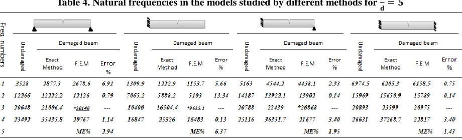
Table 4. Natural frequencies in the models studied by different methods for 𝐥
𝐝= 𝟓
Table 4 presents the investigation of the beam in four supporting conditions for the length to height ratio of l
d= 5. The
maximum considerable error value is 7% for clamped-clamped status of the beam. The sum of this error is 2.94 for three frequencies. The mode related to the axial vibration of this status is happened in the third frequency. The error level is reduced in the first frequency and increased in the third frequency for the cantilever beam due to the free fluctuation of the end beam. This much is severely reduced in the higher modes
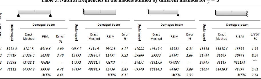
Table 5. Natural frequencies in the models studied by different methods for 𝐥 𝐝= 𝟑
Natural frequencies have been calculated for undamaged beam in the status of l
d= 3 and
presented in Table 5. The error value is lower than 5% in the first two frequencies of clamped- clamped beam. However, it is 6.48% in the third frequency of exact solution which is equivalent to the fourth frequency of finite element analysis. Mean error value (ME %) is generally 4.63. The error value increases in the cantilever status of beam like previous statuses and decreases in the simple- clamped beam up to acceptable level. In the clamped- clamped beam, maximum error value is 5.4% in both E% and ME%, indicating the high accuracy of the obtained results. The length to height ratio lowers than 3 occurs hardly in the reality. It is difficult or sometimes impossible to be measured by ordinary methods like modal hammer, concerning the increase of natural frequencies. Consequently, the results obtained in this research are valid in the length to height ratio ranges of 3-9. With increasing this ratio the measuring of frequencies is practically impossible in the beam with Euler–Bernoulli beam theory and the ratio of lower than 3.
Generally, the error value is lower than 5% in the three studied statuses for all supporting conditions, indicating the high accordance between the finite element and exact solution methods. The considerable error value is 6.37 % in the cantilever beam. This much is
ignorable considering the involved factors such as noises.
5. Numerical analysis results of with
MOGA and MMOGAThe numerical analysis method and the performance of program are confirmed by conducting the verification presented in section 3. Accordingly, this section focuses on the performances of optimization methods in the identification of exact location and intensity of the damage in different cantilever, simply supported, clamped- clamped and simply clamped beams. This method has been generalized for the length to height ratios of 3, 5, and 9.
According to Figure 2 and the general process of optimization, a beam has been considered with the cross section of 12.5×25 mm2 and a crack with half height of beam and 100 mm distance from support. It has been modeled in four different kinds with relevant supporting conditions. The first three natural frequencies are calculated in each supporting conditions. The frequencies obtained in this section are used as the input of the method suggested in this research. Then the exact location and depth of crack is identified using two optimization methods.
Figure 2. Identifying the location of structural damage in a deep beam
225mm
The previous process is repeated after identifying the location and distance of the damage with the ratios of 𝑙
𝑑=3 and 5. The
damage identification is then assessed again for four supporting conditions.
5-1. Investigating the convergence
process in the applied optimization
methods
The frequency values are practically different in each measurement due to various environmental factors such as temperature and noises existed around the structure. Therefore, meeting an accurate frequency in the identification of structural damage is not possible in the ordinary tests such as modal hammer. On the other hand, converging to a certain number is very difficult in generating through artificial intelligence methods. Therefore, the frequency ranges of ±5 have been selected as the high and low values, to consider the effects of noises as well as convergence in the optimization process.
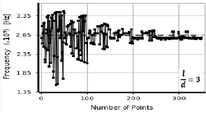
Figure 3-A. The first frequency of cantilever beam with MOGA method 𝐥
𝐝= 𝟗
Figure 3-B. The first frequency of cantilever beam with MOGA method 𝐥
𝐝= 𝟓
Figure 3-C. The first frequency of cantilever beam with MOGA method 𝐥
𝐝= 𝟑
Figure 3 presents a sample of the curves obtained from optimization process. These curves show the trial and errors performed in the optimization process. Accordingly, the horizontal axis shows several points in which the analysis has met convergence. In these analyses about 400 points are created for meeting the final response. In this method, about first 50 points are created randomly. The next generations of these data have been modified according to the explanation of section 2. After generating 8 generations, the analysis has been convergent to the response.
5-2. The results obtained from
suggested method based on MOGA
and MMOGA
Table 6. The results of optimization method through MOGA simulation in the beam with 𝐥
𝐝= 𝟗
Error % Present
Study
Exact Method
Error % Present
Study
Exact Method
Error % Present
Study
Exact Method
Error % Present
Study
Exact Method
1.49 1553.20 1530.1
0.92 975.77 966.75
0.98 2232.98 2211.2
0.87 395.24 391.78
1
0.07 5231.54 5227.8
0.06 4411.92 4409.2
0.15 6060.87 6070.2
2.87 2001.03 1943.5
2
0.30 10752.80 10721
17.37 8062.11 9462.2
0.04 11566.75 11571
0.07 6202.79 6207.2
3
0.29 99.71
100 2.70 102.78 100
20.83 126.31
100 0.88 99.13
100
Distance
3.14 12.12
12.5 0.87
12.39 12.5
4.59 11.95
12.5 5.40
11.86 12.5
Depth
Table 6 presents the results obtained from suggested method modeling for different kinds of supporting conditions in l
d= 9. In
this case, the distance of damage from support is 100 mm and its dept is 12.5mm. The distance and depth of the crack have been calculated in a cantilever beam based on the first three frequencies. The error values are 5.4% for depth and 0.88% for the
distance from support comparing to the real values. In the other words, the depth calculated by suggested method is 11.86 mm, indicating the high accuracy of the method, comparing to the real value. Similar results are obtained for simply supported and simple-clamped beams, showing high accuracy of the proposed method.
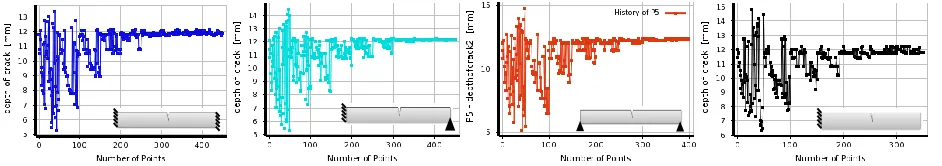
Figure 4. The process for meeting the depth of damaged beam with different supporting conditions by MOGA method for 𝐝𝐥= 𝟗
Figure 4 presents the process and value of the depth obtained for four supporting conditions. The final response in all
supporting conditions is estimated with acceptable accuracy (maximum 5%).
Figure 5. The process for meeting the distance from support in the damaged beam with different supporting conditions by MOGA method for 𝐥 𝐝= 𝟗
The error value in estimating the distance of damage from support increases and reaches to 20% in the clamped- clamped beam. The
Table 7. The results obtained from optimization method through MMOGA simulation in the beam with 𝐥 𝐝= 𝟗 Error % Present Study Exact Method Error % Present Study Exact Method Error % Present Study Exact Method Error % Present Study Exact Method 1.44 1552.49 1530.1 0.93 974.18 966.75 0.98 2226.92 2211.2 0.73 394.65 391.78 1 0.06 5230.71 5227.8 0.06 4411.74 4409.2 0.15 6077.14 6070.2 2.30 1989.28 1943.5 2 0.30 10753.6 10721 17.38 8053.52 9462.2 0.04 11570.4 11571 0.08 6202.05 6207.2 3 2.08 99 6 1 100 2.69 103.09 100 16.8 12 0 .3 0 100 0.86 99.14 100 Distance 2.56 12.19 12.5 0.88 12.34 12.5 4.54 12.09 12.5 5.39 11.86 12.5 Depth
In Table 7 presents the depth and distance from support for the beam with l
d = 9
through MMOGA method. MMOGA has been used as the second optimization method in this research. The error value has been considerably reduced particularly in the clamped- clamped beam. This fact indicates
the effectiveness of Kriging algorithm in the distribution and reduction of errors. The time needed for meeting the optimum response in this case is 0.92 of that of multi-objective genetic algorithm.
Table 8. The results obtained from optimization method through MOGA simulation in the beam with 𝐥
𝐝= 𝟓 Error % Present Study Exact Method Error % Present Study Exact Method Error % Present Study Exact Method Error % Present Study Exact Method 0.077 4441.51 4438.1 0.081 2680.78 2678.6 0.108 6165.15 6158.5 0.821 1163.25 1153.7 1 0.039 13896.64 13902 0.014 12127.7 12126 0.053 15797.3 15789 0.607 5134.14 5103 2 0.027 21682.83 21677 0.006 20768.2 20767 0.132 22847.2 22817 0.127 16462.14 16483 3 0.119 62.57 62.5 0.687 62.07 62.5 0.689 62.93 62.5 0.971 61.90 62.5 Distance 0.947 12.38 12.5 0.591 12.43 12.5 0.799 12.40 12.5 1.981 12.26 12.5 Depth
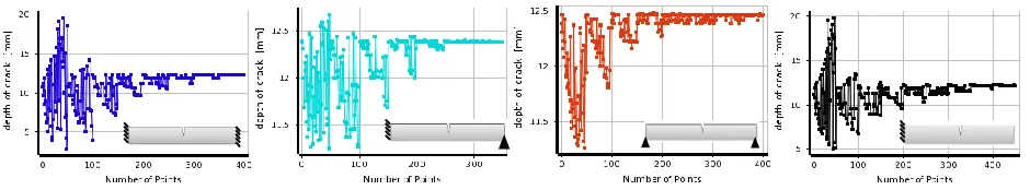
Table 8 presents the depth and distance from support for the deep beam with l
d= 5
through MOGA. The whole length of beam is 125mm; the damage is located at the distance of 62.5mm from support. The depth of damage is equal to the half of the beam height. With decreasing the beam length and
approaching the behavior from Euler– Bernoulli beam theory toward theory, the error values calculated for measuring the depth and distance from support is significantly reduced. Accordingly, maximum evaluated error value is 2%.
Figure 6 presents the trend of meeting optimum response in four supporting conditions. According to Figures 6 and 7, the primary responses are very different form final response in the first 50- data range. By generating 7-9 generations, there will be
350-450 sample responses, approaching towards final response with great accuracy. The trend of meeting optimum response has been assessed in four supporting conditions and presented in Figure 7.
Figure 7. The process for meeting the distance from support in the damaged beam with different supporting conditions by MOGA method for 𝐥
𝐝= 𝟓
Table 9 presents the efficiency of suggested method in detecting the distance and depth parameters for different kinds of supporting conditions in the beam with l
d= 5 through
MMOGA method. No siginificat error is observed between the optimum responses of
MOGA and MMOGA methods, considering both parameters. Maximum error value is corresponded to the status of l
d= 9 in
detecting the damage distance. The time needed for meeting optimum response in MMOGA method is 82% of that of MOGA.
Table 9. The results obtained from optimization method by MMOGA simulation in the beam with 𝐥
𝐝= 𝟓
Error % Present
Study
Exact Method
Error % Present
Study
Exact Method
Error % Present
Study
Exact Method
Error % Present
Study
Exact Method
0.076 4441.46
4438.1 0.081
2679.60 2678.6
0.108 6166.07 6158.5
0.824 1163.29
1153 1
0.039 13896.57 13902
0.014 12124.6 12126
0.053 15797.1 15789
0.612 5134.40
5103 2
0.026 21682.59 21677
0.006 20769.4 20767
0.132 22853.1 22817
0.127 16462.14 16483
3
0.119 62.57
62.5 0.687 62.03
62.5 0.690 62.81
62.5 0.971 61.90
62.5 Distance
0.957 12.38
12.5 0.589 12.47
12.5 0.802 12.36
12.5 1.981 12.26
12.5 Depth
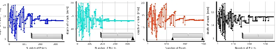
Table 9 shows the depth and distance from support in different kinds of supporting conditions for the beam with l
d= 3 through
MOGA method. In ths case, the length of beam is 75mm, the distance of damage location from support 37.5 mm and its depth
Table 10. The results obtained from optimization method through MOGA simulation in the beam with 𝐥
𝐝= 𝟑
Error % Present
Study Exact
Method Error
% Present
Study Exact
Method Error%
Present Study Exact
Method Error%
Present Study Exact
Method
0.052 10316.59 10322
1.499 6414.43 6510.6
0.288 13859.
13899 5.711
2779.56 2938
1
0.874 28597.00 28847
1.174 26081.7 26388
0.613 30759
30948 12.923 10181.28
11497 2
0.764 40492.58 40802
0.665 39686.2 39950
17.894 35196
41494 1.960
31806.61 32430
3
1.89 38.23
37.5 3.658 38.92
37.5 1.527
36.94 37.5
2.290 36.66
37.5 Distance
5.65 13.25
12.5 5.966 13.29
12.5 5.306
13.20 12.5
5.661 13.25
12.5 Depth
Table 10 presents maximum error value occurred in the calculation of the third frequency for clamped- clamped beam. This error is due to the interference of flexural and axial modal shape. The error values in
calculating the two mentioned parameters are reduced up to about 5.3% with respect to applying the first three frequencies as the input of optimization process.
Figure 8. The process for meeting the depth in the damaged beam for different supporting conditions by MOGA method for 𝐥
𝐝= 𝟑
Figures 8 and 9 have shown the trend of meeting optimum response of depth and distance from support in different kinds of supporting conditions for length to height ratio of 3 in MOGA method. According to
Figures 4-9, higher error values are observed in the convergence trend for determining the distance from support, comparing to that of depth parameter due to the significant effect of different distances on natural frequencies.
Figure 9. The process for meeting the distance from support in the damaged beam for different supporting conditions by MOGA method for 𝐥 𝐝= 𝟑
Table 11 presents the depth and distance from support in different kinds of supporting conditions for the beam with l
d= 3 through
MMOGA method. The calculated error value is lower in this method comparing to its corresponding status, indicating high
Table 11. The results obtained from optimization method through MMOGA simulation in the beam with 𝐥 𝐝= 𝟑 Error % Present Study Exact Method Error % Present Study Exact Method Error % Present Study Exact Method Error % Present Study Exact Method 0.198 10301.59 10322 1.497 6426.12 6510.6 0.288 13859.44 13899 5.919 2774.09 2938 1 0.898 28590.23 28847 1.170 26173.0 26388 0.612 30800.03 30948 12.93 10180.02 11497 2 0.891 40441.70 40802 0.666 39627.2 39950 15.32 41104.24 41494 1.804 31855.26 32430 3 1.577 38.10 37.5 3.720 38.27 37.5 1.511 37.34 37.5 1.870 36.81 37.5 Distance 5.719 13.26 12.5 4.71 13.12 12.5 4.79 13.13 12.5 0.95 13.2 12.5 Depth
Optimization has been performed for four kinds of supporting conditions including cantilever, clamped- clamped, simply supported and simple clamped beams. This process has been assessed for length to depth ratios of 5, 3, and 9, using MMOGA and MOGA methods. Totally 48 analyses have been conducted for all statuses. The evaluated error value has been approximately lower than 5% in all statuses, excluding clamped- clamped beam, for two studied parameters. However, this error value is about 20% for clamped-clamped beam in the multi-objective genetic algorithm and 16% in the modified multi-objective genetic algorithm due to the high entered noised and axial and flexural modal shapes.
6. Investigating an applicable
example using the results of
suggested method
The proposed method has been assessed in the previous discussion. The performance of the method has been verified by the final responses and its accuracy by the results obtained for all statuses. According to Figure 3, the general trend of solving the problem has been studied for different kinds of supporting conditions. Therefore, the problem can be solved to meet the optimum response in this example.
6-1. The specifications of studied
sample
In this example the considered beam has the elastic module of 200 (GPa), material mass density of 7860 kg/ m3 and poison ratio of 0.3. This problem has been assessed for cantilever, simply supported, clamped-clamped, and simple-clamped supporting statuses of beam.
Figure 10. A sample of supporting condition and the
crack location in the studied beam
The dimensions of beam are shown in Figure 10. It has the width of 1000 mm, height of 200 mm and length of 2000 mm with the ratio of l
d= 10. The location and depth of
crack are 1000 mm and 100 mm, respectively.
Table 12. The results of first three natural frequencies in
numerical method for all cracked beams
The first three frequencies are obtained for four supporting statuses using numerical method and presented in Table 14. Maximum noises considered for solving the problem is 5%. The results of suggested method are assessed in the following.
6-2. The distribution of damage
locations after optimization process
The suggested method has been applied for all supporting statuses. The obtained results might be similar to the real responses. Accordingly, the optimization may present one or more responses at the end of convergence process. Different responses have been obtained from the analyses, presented in the tables, after optimization process. However, the optimum response has been assessed concerning high volume of the results. Regarding the high volume of calculations as well as the similarity between the results of MOGA and MMOGA, only one optimization method has been investigated and presented in Figures 11-18. This can be generalized in all statuses.
Figure 11-A. The location obtained after optimization process in the cantilever beam
Figure 11-B. The depth of crack obtained after optimization process in the cantilever beam
According to Figure 11, three points have been obtained, coincident with the specifications of analysis input, after optimization process. In this figure the vertical axis shows the accordance between the optimization and real responses. The left to right directions of horizontal axis shows length and depth of the beam, respectively. In this figure, two points obtained from optimization process are related to the depth and distance of the damage, agreed with the real responses up to about 95%. Another response is corresponded to the damage location with 1850mm distance and 45mm depth. The accumulation of responses in this process indicates the high accuracy of optimization process.
Figure 12-A. The locations obtained after optimization process in the clamped- clamped
beam 0 10 20 30 40 50 60 70 80 90 100 0 1 0 0 2 0 0 3 0 0 4 0 0 5 0 0 6 0 0 7 0 0 8 0 0 9 0 0 1 0 0 0 1 1 0 0 1 2 0 0 1 3 0 0 1 4 0 0 1 5 0 0 1 6 0 0 1 7 0 0 1 8 0 0 1 9 0 0 Per ce n tag e o f Dama ge De te cti o n Beam Length(mm) 0 10 20 30 40 50 60 70 80 90 100
0 10 20 30 45 50 60 70 80 90
10 3 1 0 9 1 2 0 1 3 0 1 4 0 1 5 0 1 6 0 1 7 0 1 8 0 1 9 0 2 0 0
Depth of Crack(mm)
Per ce n tag e o f Dama ge De te cti o n 0 10 20 30 40 50 60 70 80 90 100 0 1 0 0 2 0 0 3
00 400 500 006 700 800 900
Figure 12-B. The depth of crack obtained after optimization process in the clamped- clamped
beam
The location and depth of clamped-clamped beam have been presented in Figure 12. In this figure, two points with 1000 mm distance and 100 mm depth are 100% in accordance with real response. Another point with 1200 mm distance and 123 mm depth agrees with real response about 65%. By the way, the other location and depth of the damage can easily be detected.
Figure 13-A. The locations obtained after optimization process in the simply supported beam
Figure 13. The depth of crack obtained after optimization process in the simply supported beam
The optimization results of clamped- clamped and simple- clamped beams are presented in Figures 13 and 14, respectively. According to Figure 14, the responses of the suggested numerical method are totally in agreement with the real value, showing the high accuracy of the software.
Figure 14-A. The locations obtained after optimization process in the simple- clamped beam
Figure 14-B. The depth of crack obtained after optimization process in the simple- clamped beam 0 10 20 30 40 50 60 70 80 90 100
0 10 20 30 45 50 60 70 80
9 9 .9 5 1 0 0 1 1 0 1 2 3 .1 1 1 3 0 1 4 0 1 5 0 1 6 0 1 7 0 1 8 0 1 9 0 2 0 0
Depth of Crack(mm)
Per ce n tag e o f Dama ge De te cti o n 0 10 20 30 40 50 60 70 80 90 100 0 1 0 0 2 0 0 3
00 004 500 600 070 800 900
1 0 0 0 1 1 0 0 1 2 0 0 1 3 0 0 1 4 0 0 1 5 1 2 1 6 0 0 1 7 0 0 1 8 0 0 1 9 0 0 Per ce n tag e o f Dama ge De te cti o n Beam Length(mm) 0 10 20 30 40 50 60 70 80 90 100
0 10 20 30 40 50 60 70 80 99
1 0 3 1 1 0 1 2 0 1 3 0 1 4 5 1 5 0 1 6 0 1 7 0 1 8 0 1 9 0 2 0 0
Depth of Crack(mm)
Per ce n tag e o f Dama ge De te cti o n 0 10 20 30 40 50 60 70 80 90 100 0 1 0 0 2 0 0 3 0 0 4 0 0 5 0 0 6 0 0 7 0 0 8 0 0 9 0 0 1 00 0 1 1 0 0 1 2 0 0 1 3 0 0 1 4 0 0 1 5 0 0 1 6 0 0 1 7 0 0 1 8 0 0 1 9 0 0 Per ce n tag e o f Dama ge De te cti o n Beam Length(mm) 0 10 20 30 40 50 60 70 80 90 100
0 10 20 30 40 50 60 70 80 92 93
1 1 0 1 2 0 1 3 1 1 4 5 1 5 0 1 6 0 1 7 0 18 0 1 9 0 2 0 0
Depth of Crack(mm)
6. Conclusion
So far the identification of damages in the structures were presented by composing two or more parameters including natural frequencies, modal shape, curvature of modal shape, energy of modal strain, residual force vector, modified matrix and frequency response function. This research focuses on identifying the exact location of damage using optimization methods and based only on the first three frequencies of deep beams. Natural frequencies are easily calculated in the first modes of different structures by simple tests such as modal hammer. The method suggested in this study presents an effective step in the identification of exact location and depth of damage. Another advantage of the proposed method is its capability in the determination of depth and fissure of the damage resulting in the calculation of its intensity. The results obtained in this research indicated the capability of suggested method. Here, the new method has been used to identify the damages in the structures. For this purpose 84 analyses was conducted, out of which 36 and 48 analyses for verifying the results of finite element and proposed methods, respectively. The obtained results confirm the capability of this new method in identifying the damages of structures and most particularly in the deep beam shape structures. In the ordinary structures, one of the first frequencies is axial mode with flexural behavior, concerning the ref. [21]. On the other hand, axial frequency cannot be measured in the beams by ordinary devices. Axial mode, measurable in the finite element analysis, has been ignored in this research. The time needed for analysis and meeting the convergence are of the most important factors, considering the numerical method results in the convergence process. The time needed for performing optimization with
MOGA and MMOGA methods was
investigated confirming the lower duration of MMOGA in comparison with the other one.
The error level is lower than 5% excluding the clamped-clamped supporting status of beam in which the error value increases considering the vicinity of natural frequencies in the near locations and depts. MMOGA method presents better responses in a specific status, comparing to MOGA. In such cases the error level decreases from 20% to 16% in the most critical status (clamped- clamped) due to the distribution and error finding of Kriging algorithm. These two methods were assessed in order to meet the real responses with minimum error values. Each or both methods can present real responses in different conditions. Maximum values of calculated error of final response after optimization process have been 6% in the depth of crack for all supporting statuses, considering the ratio of length to depth of sample as 3. The rate of error increases in the determination of distance parameter as the mentioned ratio increases to 9. Therefore, it can be concluded that the studied method has high accuracy for Timoshenko beams with respecting the length to thickness ratios lower than 5. The existence of noises is inevitable in the experiments. They are formed due by the environmental vibrations, temperature, register system vibrations, measurement errors and so on. The created noises level has been considered as 5% and their effects as 95% - 105% of the values of real frequency in the optimization process.
7. Reference
[1]. ASTMC1383-04, A., Standard test method for measuring the P-Wave speed and the thickness of concrete plates using
the impact-echo method. 2010, American
[2]. ASTM, C., Standard test method for
pulse velocity through concrete. Annual
Book of ASTM Standards, American Society of Testing Material, 2009.
[3]. Amezquita-Sanchez, J.P. and H. Adeli, Signal processing techniques for
vibration-based health monitoring of smart
structures. Archives of Computational
Methods in Engineering, 2016. 23(1): p. 1-15.
[4]. Zhao, B., et al., Structural Damage Detection by Using Single Natural Frequency and the Corresponding Mode
Shape. Shock and Vibration, 2016. 2016.
[5]. Goldfeld, Y. and D. Elias, Using the exact element method and modal frequency changes to identify distributed damage in beams. Engineering Structures, 2013. 51: p. 60-72.
[6]. Perera, R., R. Marin, and A. Ruiz, Static– dynamic multi-scale structural damage
identification in a multi-objective
framework. Journal of Sound and
Vibration, 2013. 332(6): p. 1484-1500. [7]. Mehrjoo, M., N. Khaji, and M.
Ghafory-Ashtiany, Application of genetic algorithm in crack detection of beam-like structures using a new cracked Euler–Bernoulli beam
element. Applied Soft Computing, 2013.
13(2): p. 867-880.
[8]. Moradi, S., P. Razi, and L. Fatahi, On the application of bees algorithm to the problem of crack detection of beam-type structures. Computers & Structures, 2011.
89(23): p. 2169-2175.
[9]. Zang, C. and M. Imregun, Structural damage detection using artificial neural networks and measured FRF data reduced
via principal component projection.
Journal of Sound and Vibration, 2001.
242(5): p. 813-827.
[10].Meruane, V. and W. Heylen, An hybrid real genetic algorithm to detect structural
damage using modal properties.
Mechanical Systems and Signal Processing, 2011. 25(5): p. 1559-1573.
[11]. Ghasemi, S.H. and P. Ashtari, Combinatorial continuous non-stationary critical excitation in MDOF structures
using multi-peak envelope functions.
Earthquakes and Structures, 2014. 7(6): p. 895-908.
[12].Farokhzad Reza, M.B., Ghodrati Amiri Gholamreza, Ghafory-Ashtiany Mohsen,
Detecting structural damage in
Timoshenko beams based on optimization
via simulation (OVS). Journal of
Vibroengineering, 2016. 18(8): p. 5074-5095.
[13].Altammar, H., S. Kaul, and A. Dhingra. Use of Frequency Response for Damage
Detection: An Optimization Approach. in
ASME 2016 International Design
Engineering Technical Conferences and Computers and Information in Engineering
Conference. 2016. American Society of
Mechanical Engineers.
[14].Hjelmstad, K. and S. Shin, Crack identification in a cantilever beam from modal response. Journal of Sound and Vibration, 1996. 198(5): p. 527-545. [15].Ghasemi, S.H., et al., State-of-the-art
model to evaluate space headway based on
reliability analysis. Journal of
Transportation Engineering, 2016: p. 04016023.
[16]. Koh, B., J. Choi, and M. Jeong. Damage Detection through Genetic and
Swarm-Based Optimization Algorithms. in
International Conference on Engineering, Science, Construction and Operations in Challenging Environments. International Conference on Engineering, Science,
Construction and Operations in
Challenging Environments. 2010.
[17].Law, S., Z. Shi, and L. Zhang, Structural damage detection from incomplete and
noisy modal test data. Journal of
Engineering Mechanics, 1998. 124(11): p. 1280-1288.
[19].Tada, H., P. Paris, and G. Irwin, The
analysis of cracks handbook. 2000: New
York: ASME Press.
[20].Petyt, M., Introduction to finite element
vibration analysis. 2010: Cambridge
university press.
[21].Khaji, N., M. Shafiei, and M. Jalalpour, Closed-form solutions for crack detection problem of Timoshenko beams with various boundary conditions. International Journal of Mechanical Sciences, 2009. 51(9): p. 667-681.
[22].Ostachowicz, W. and M. Krawczuk, Analysis of the effect of cracks on the natural frequencies of a cantilever beam. Journal of sound and vibration, 1991.