Estimation of xanthate decomposition percentage as a function of pH, temperature and time by least squares regression and adaptive neuro-fuzzy inference system

* Corresponding author. Tel. +98-9151603400, E-mail address: [email protected] (A. Behnamfard).

Journal Homepage: ijmge.ut.ac.ir

Estimation of xanthate decomposition percentage as a function of pH,

temperature, and time by least squares regression and adaptive

neuro-fuzzy inference system

Ali Behnamfard

_{, Francesco Veglio}

a _{Faculty of Engineering, University of Birjand, Birjand, South Khorasan, Iran}

a _{Department of Industrial and Information Engineering and Economics, University of L’Aquila, Monteluco di Roio, L’Aquila, Italy}

ABSTRACT

Estimating the xanthate decomposition percentage has a crucial role in the treatment of xanthate contaminated wastewaters and in the improvement of the flotation process performance. In this research, the modeling of xanthate decomposition percentage was performed using the least squares regression method and the Adaptive Neuro-Fuzzy Inference System (ANFIS). A multi-variable regression equation and the ANFIS models with various types and numbers of membership functions (MFs) were constructed, trained, and tested for the estimation of xanthate decomposition percentage. The statistical indices such as Root Mean Squared Error (RMSE), Mean Absolute Percentage Error (MAPE), and coefficient of determination (R2_{) were used to evaluate the performance of various models. The lowest values of RMSE and} MAPE and the closest value of R2 _{to unity were determined for the ANFIS model with the triangular membership function and the number} of input MFs 9 9 9 (0.766906, 3.553509 and 0.998793). This indicates that ANFIS is a powerful method in the estimation of xanthate decomposition percentage. The performance of new-adopted ANFIS data modeling was significantly better than the conventional least squares regression method.

Keywords : Xanthate, Decomposition percentage, Estimation, ANFIS, Regression

1.

Introduction

The flotation process is widely used to up-grade base metal sulfide ores [1]. Annually, billion tons of sulfide ores are treated through this separation method and a huge amount of xanthate is used as the collecting agent in the flotation process [2]. Xanthates have a heteropolar molecular structure with a nonpolar hydrocarbon group and a polar head [2]. An electrochemical reaction occurs between the sulfide mineral surface and the polar head of xanthate [3]. This reaction makes the surface of sulfide minerals hydrophobic and it allows these mineral particles to be floated by air bubbles and be separated from other hydrophilic gangue minerals [4]. The dosage of xanthate in the flotation process varies in the range of 50 to 350 gr per ton of ore treated [5].

Decomposition percentage of xanthate can be determined through the following equation:

0 % (1 Ct) 100 Decomposition

C

   (1)

where C0 (mg/L) is the initial concentration of xanthate in the solution and Ct (mg/L) is the xanthate concentration in the solution at time t.

The decomposition of xanthate in the flotation pulp can reduce its effective concentration [6]. The effective concentration of xanthate in the flotation pulp plays a crucial role in the floatability of sulfide minerals [6]. Furthermore, the decomposition products of xanthate can

reduce the selectivity of a flotation process [6]. The stability of xanthate in aqueous solutions depends on several factors, especially the solution pH and temperature [6, 7]. In acidic aqueous solutions, xanthate undergoes hydrolysis to xanthic acid (ROCS2H) which decomposes into carbon disulphide (CS2) and alcohol (ROH) according to the following equations [8]:

ROCS2- + H2O → ROCS2H + OH- ₍₂₎

ROCS2H → CS2 + ROH (3)

In neutral and alkaline media, the decomposition of xanthate occurs through hydrolytic decomposition according to the following reaction [8]:

6ROCS2- + 3H2O → 6ROH + CO32- + 3CS2 + 2CS32- (4) As the solution temperature increases, the decomposition percentage of xanthate increases as well [9]. This is important due to the fact that the flotation of sulfide minerals is performed at various pulp temperatures during the summer and winter [6].

Although xanthates react selectively with the mineral surfaces in the ore pulp and are utilized at optimum dosages, excess and unreacted concentrations of these organosulfur compounds end up into the plant effluents [8]. Xanthates are toxic to aquatic life and therefore the release of xanthate contaminated wastewaters into the environment has sever environmental problems [10]. In recent years, several methods have been developed to remove xanthate from wastewaters, such as adsorption [10], chemical precipitation [11], chemical oxidation [8, 12-14], biodegradation [15, 16]. In natural degradation, chemical oxidation and biodegradation methods, the removal of xanthate is usually

performed through accelerating the degradation kinetics.

The estimation of xanthate decomposition percentage is highly crucial in sulfide mineral flotation and in the treatment of xanthate contaminated wastewaters, but it has not received enough attention up to now. In this research, we initially try to establish an equation for the estimation of xanthate decomposition percentage based on the process parameters including pH, temperature, and time by using the conventional least squares regression method. For this reason, the initially best subsets regression was applied using Minitab 17 software to identify a model with as few variables as possible and then the regression model was developed by multivariable regression. In this study, we also try to model the xanthate decomposition percentage by a new-adopted ANFIS data modeling procedure. ANFIS was first introduced by J. Jang in 1993 [17]. It is an artificial neural network that is based on the Takagi–Sugeno fuzzy inference system [17]. ANFIS has the potential to capture the benefits of both neural networks and the fuzzy logic in a single framework since it integrates the principles of both methods [18, 19]. ANFIS can be considered as a universal estimator since its inference system corresponds to a set of fuzzy IF–THEN rules that have a learning capability to approximate nonlinear functions [18, 19].

2.

Methodology

2.1.Data

Table 1 shows the statistical parameters of the input and output data. The available dataset consisting of 1160 records was randomly divided into two subsets, the training set, and the testing set. Totally, 80% of the dataset (80%=929 data sets) was utilized for training the model and the remainder data points (20% =231 data sets) were utilized for the testing procedure. The datasets were extracted from previously published papers [6-9, 20-23].

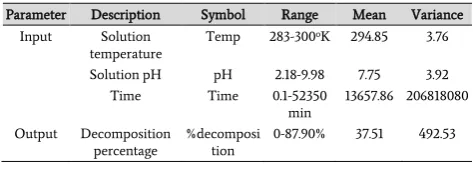
Table 1. Description of input and output parameters in ANFIS and regression models.

Parameter Description Symbol Range Mean Variance Input Solution

temperature Temp 283-300

o_{K 294.85 3.76}

Solution pH pH 2.18-9.98 7.75 3.92 Time Time 0.1-52350

min 13657.86 206818080 Output Decomposition

percentage %decomposition 0-87.90% 37.51 492.53

2.2.Adaptive neuro-fuzzy inference system (ANFIS)

To describe an ANFIS system, it is simply surmized that the inference system has two inputs x and y and one output f. A first-order Sugeno fuzzy model has two rules as the following:

Rule 1. If x is A1 and y is B1, then f1 = p1x +q1y + r1. (5) Rule 2. If x is A2 and y is B2, then f2 = p2x +q2y+ r2. (6) where p1, p2, q1, q2, r1 and r2 are linear parameters in the consequent part and A1, A2, B1 and B2 are nonlinear parameters [24].

Fig. 1 illustrates the corresponding equivalent ANFIS architecture for two input first-order Sugeno fuzzy model with two rules. The entire system architecture consists of five layers, including the fuzzy layer, product layer, normalized layer, de-fuzzy layer, and total output layer [25]. The node functions in the same layer are of the same function family as described in the following:

Layer 1: this layer is called the fuzzy layer. The adjustable nodes in this layer are represented by the square nodes and marked by A1, A2, B1 and B2 with x and y outputs. A1, A2, B1 and B2 are the linguistic labels (small, large, etc.) used in the fuzzy theory for dividing the MFs. The node functions in this layer that determine the membership relation between the input and output functions can be given by:

2

1,

1,

( ), 1, 2 ( ), 3, 4

i

i

i A

i B

O x i

O y i

  

 

  (7)

where O1,i and O1,j denote the output functions, and µAi(x) and µBi-2(y) denote the appropriate MFs, which could be triangular, trapezoidal, Gaussian, generalized bell functions [24]. The MFs are defined as follows:

A triangular MF is specified by three parameters {a, b, c} as follows [25]:

 

a x b

b a

x

c x

b x c

c b c x             _  _{ }    _  (8)

The parameters {a, b, c} (with a < b < c) determine the x coordinates of the three corners of the underlying triangular MF.

A trapezoidal MF is specified by four parameters {a, b, c, d} as follow [25]:

 

a x b

b a

x b x c

d x

c x d

d c d x                         (9)

The parameters {a, b, c, d} (with a < b <= c < d) determine the x coordinates of the four corners of the underlying trapezoidal MF. A Gaussian MF is specified by two parameters as follows [25]:

  2

2 ( ) exp( ) 2 i A x c x   

  (10)

A Gaussian MF is determined complete by c and σ; c represents the MFs center and σ determines the MFs width.

A generalized bell MF is specified by three parameters {a, b, c} as follows [24]:

  2

1 1

i

A x b

x c a       _ _ (11)

where parameter b is usually positive.

Layer 2: this is the product layer and each node is a fixed node marked by a circle node and labeled by Prod. The outputs w1 and w2 are the weight functions of the next layer. The output of this layer, O2,i, is the product of all incoming signals and is given by:

2,i i Ai( ) Bi( ), 1, 2

O w  x  y i (12)

The output signal of each node, wi, represents the firing strength of a rule [24].

Layer 3: this is the normalized layer and each node in this layer is a fixed node, marked by a circle node and labeled by Norm. The nodes normalize the firing strength by estimating the ratio of firing strength for this node to the sum of all firing strengths, i.e.

3,

1 2 , 1, 2.

i

i i

w

O w i

w w

  

 (13)

Layer 4: This is the de-fuzzy layer having adaptive nodes and marked by square nodes. Each node i in this layer is an adaptive node with a node function:

4,i i i i( i i i), 1, 2

O w f w p xq yr i (14)

where wi is the normalized firing strength output from layer 3 and

pi, qi and ri are the parameters set of this node. These parameters are linear and referred as consequent parameters of this node [24].

5,

1 2 , 1, 2

i i

i i i

i

w f

O w f i

w w

  







Fig 1. An ANFIS network structure for a simple FIS.

An ANFIS network can be trained based on supervised learning to reach from a specific input to a definite target output. In the forward pass of the hybrid algorithm of ANFIS, the node outputs go forward until the fourth layer and consequent linear parameters, (pi, qi, ri), are found by the least-squares method using the training dataset. The error signals propagate backwards in the pass and the premise nonlinear parameters, (ai, bi, ci) are updated by the gradient descent. It has been proven that this hybrid algorithm is highly efficient in training ANFIS models [26].

2.3.Development of ANFIS models

To model the decomposition percentage of xanthate, a network with three inputs was selected, with input variables corresponding to the solution temperature, pH, and time (Fig. 2).

Fig 2. System ANFIS: 3 inputs (Temperature, pH, and Time), 1 output (decomposition percentage)

The applicability of ANFIS models to estimate the decomposition percentage of xanthate was validated by the following criteria:

Root Mean Squared Error (RMSE) [27]:

2 1 1 ( ) N t t t

RMSE A F

N 





where At and Ft are actual and predicted values, respectively, and N is the number of training or testing samples.

Mean Absolute Percentage Error (MAPE) [27]:

1 1 100 N t t t t A F MA PE

N  A







Coefficient of determination (R2_{) [27]:}

2 2 1 2 1 ( ) 1 ( ) N t t t n t t A F R A A      









testing datasets. The lower RMSE and MAPE values and closer R2 _value to unity mean better performance of the models.

The best subsets regression approach is an efficient way to identify the models that achieve our goals with as few predictors as possible. This method identifies the subset models that produce the highest R2 _values from a full set of the predictor variables that we specify. Subset models may actually estimate the regression coefficients and predict future responses with smaller variance than the full model using all predictors

[28]. Minitab examines all possible subsets of the predictors, beginning with all models containing one predictor, and then all models containing two predictors, and so on [28]. Table 2 shows the results of best subsets regression performed by Minitab 17. Each row in the table represents information about one of possible regression models. The first column— labeled Vars—shows how many predictors are in the model. The last three columns show which predictors are in the model. If an "X" appears in the row, it will include in the model as the predictor. The other five columns—labeled R2_{, R}2 _{(adj), R}2 _{(pred), Cp, and S— pertain to the} criteria that we use in deciding which models are "best."

3.

Results and Discussion

3.1.Estimation of xanthate decomposition percentage by Least Square Regression Method

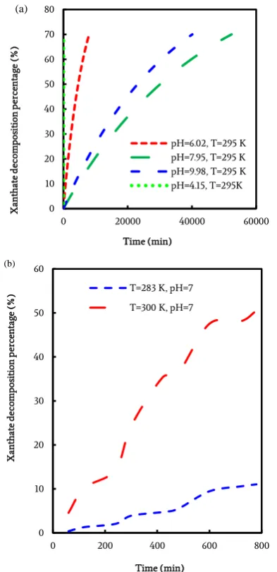
The effect of solution pH and temperature on the decomposition rate of xanthate is shown in Fig. 3. As seen, the decomposition rate of xanthate increases by increasing the solution temperature. The decomposition rate of xanthate drastically increases by decreasing the solution pH from 7.95 to 4.15 and to a lesser extent by increasing the solution pH from 7.95 to 9.95.

Fig 3. The effect of a) solution pH and b) solution temperature on the decomposition rate of xanthate

The model with all the variables has the highest R2 _{(58%) and} adjusted R2 _{(57.9%), and the lowest Mallows' Cp value (4.0) and S value}

0 10 20 30 40 50 60 70 80

0 20000 40000 60000

X an th ate d ec om po sitio n pe rc en ta ge ( % ) Time (min)

pH=6.02, T=295 K pH=7.95, T=295 K pH=9.98, T=295 K pH=4.15, T=295K (a) 0 10 20 30 40 50 60

0 200 400 600 800

X an th ate d ec om po sitio n pe rc en ta ge ( % ) Time (min) T=283 K, pH=7 T=300 K, pH=7

(14.402). Hence, the model with all the variables can be considered as the best model for the estimation of xanthate decomposition percentage at different solution conditions.

Table 2 The results of best subsets regression

Vars R2 _R2 _{(adj) R}2 _{(pred) Mallows Cp S Temp pH Time}

1 40.8 40.8 40.7 473.9 17.084 X

2 1.8 1.7 1.5 1550.8 22.013 X

3 0.6 0.5 0.2 1583.9 22.148 X

4 57.3 57.2 57.1 22.6 14.523 X X

5 41.6 41.5 41.3 455.4 16.984 X X 6 2.4 2.3 2.0 1534.8 21.950 X X 7 58.0 57.9 57.8 4.0 14.402 X X X The general regression was applied by Minitab 17 to fit least squares models to understand the relationship between the decomposition percentage of xanthate and the predictors' variables including temperature, pH, and time. Eq. 19 shows the relevant equation.

Decomposition % = 0.24298 Temp – 26.1 pH – 0.205 Time + 0.0654 Temp*pH + 0.000692 Temp*Time + 0.000283 pH*Time

(19)

Table 3 shows the analysis of variance (ANOVA) table and the model summery for the multi-variable regression model. As can be seen, the p-value for the regression model is 0.000 in the ANOVA table which indicates that the equation is statistically significant at an α-level of .05. Furthermore, the value of R2_{, R}2 _{(adj), and R}2 _{(pred) is 0.9041, 0.9036,} and 0.9031, respectively. These values are close to unity which further confirm that the model is significant at 95% confidence level for the estimation of xanthate decomposition percentage.

Table 3 ANOVA table and the model summary for the multi-variable regression model.

Analysis of Variance

Source DF Adj SS Adj MS F-Value P-Value

Regression 6 1993645 332274 1815.09 0.000

Temp 1 255187 255187 1393.99 0.000

pH 1 463 463 2.53 0.112

Time 1 135 135 0.74 0.391

Temp*pH 1 253 253 1.38 0.240

Temp*Time 1 133 133 0.73 0.394

pH*Time 1 28288 28288 154.53 0.000

Error 1155 211437 183

Total 1161 2205081

Model Summary

S R-sq R-sq(adj) R-sq(pred)

13.5300 90.41% 90.36% 90.31%

Coefficients

Term Coef SE Coef T-Value P-Value VIF

Temp 0.24298 0.00651 37.34 0.000 23.35

pH -26.1 16.4 -1.59 0.112 109208.27

Time -0.205 0.239 -0.86 0.391 1.42938E+08

Temp*pH 0.0654 0.0557 1.17 0.240 109252.52

Temp*Time 0.000692 0.000811 0.85 0.394 1.42936E+08

pH*Time 0.000283 0.000023 12.43 0.000 100.06

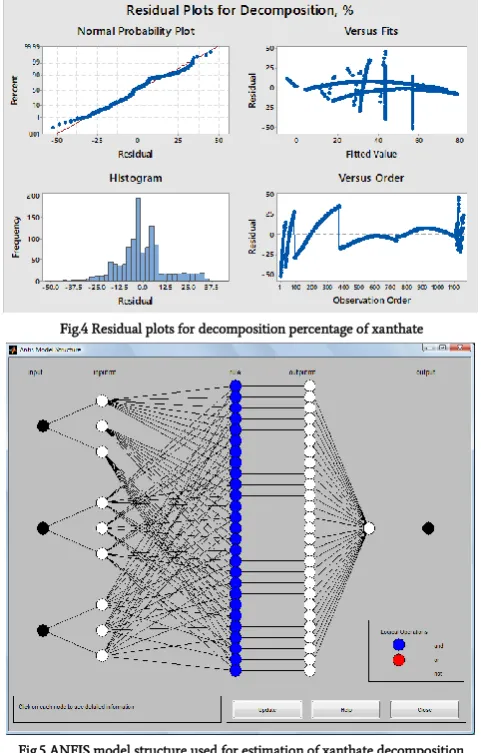
In order to further validate the relevant equation, the histogram and the normal probably plot of residuals, the plot of residual versus fitted values and the plot of residual versus the run order were plotted (Fig. 4). The histogram of residuals has a bell shape which confirms the normal distribution of the residuals. The normal probability plot shows an approximately linear pattern which is consistent with normal distributions. The plot of residual versus fitted values shows a random pattern, which confirms the constant variance of the residuals. The residual versus order plot displays the order that the data was collected and can be used to find the non-random error, especially of time-related effects. The residual versus order plot shows a random pattern which indicates the time-independent variance of residuals.

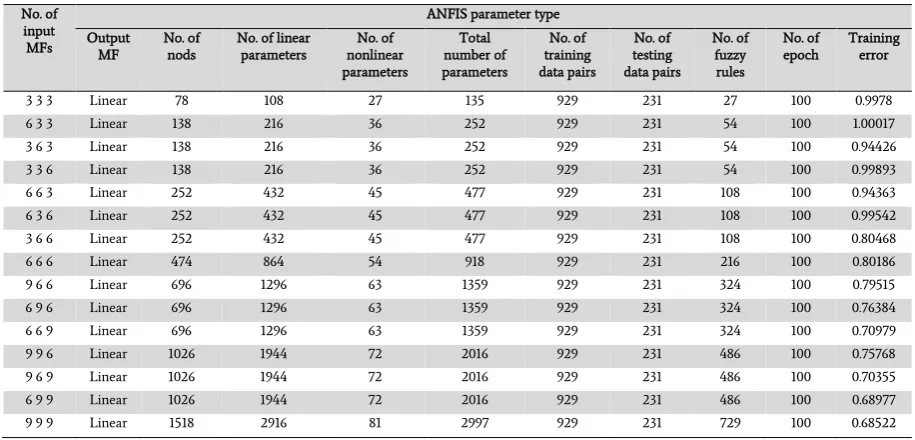
3.2.The estimation of xanthate decomposition percentage by ANFIS In this research, a hybrid grid partitioning ANFIS was applied for the estimation of xanthate decomposition percentage as a function of solution temperature, pH, and time. To evaluate the effect of MF type on the performance of ANFIS models, it was set as Triangular, Trapezoidal, Generalized bell, and Gaussian. The number of input MFs was set 3 3 3. Fig. 5 shows the general structure of ANFIS models. The characteristics of ANFIS models are shown in Table 4.

Fig.4 Residual plots for decomposition percentage of xanthate

Fig.5 ANFIS model structure used for estimation of xanthate decomposition percentage

Table 4 Parameter types of ANFIS models with different MF types.

ANFIS parameter type Membership Function Type Triangular Trapezoidal Generalized bell Gaussian Number of MFs

Output MF Number of nods Number of linear parameters Number of nonlinear parameters Total number of parameters Number of training data pairs Number of testing data pairs Number of fuzzy rules Number of epochs Training error

3 3 3 Linear

78 108 27 135 929 231 27 100 0.9978

3 3 3 Linear

78 108 36 144 929 231 27 100 4.4248

3 3 3 Linear

78 108 27 135 929 231 27 100 1.378

3 3 3 Linear

78 108 18 126 929 231 27 100 1.34923

percentage of xanthate than the other ANFIS models.

Table 5 Performances of ANFIS models with different MFs in estimation of xanthate decomposition percentage

Membership

function _{RMSE MAPE (%)} Training data set _R2 _{RMSE MAPE (%)} Testing data set _R2

Triangular 0.997799 5.114386 0.997986 1.052606 6.403248 0.997726 Trapezoidal 4.424813 119.5478 0.960386 4.279191 101.7817 0.962419 Gaussian 1.34923 7.374592 0.996317 1.284703 7.389331 0.996613 Generalized bell 1.378041 9.23183 0.996158 1.31637 8.902129 0.996444

Fig. 6 shows the applicability of ANFIS models by different MF types for the estimation of xanthate decomposition percentage. The ANFIS model with triangular MF is clearly the most accurate and powerful method for the estimation of xanthate decomposition percentage.

In order to evaluate the effect of number of input MFs on the performance of ANFIS models, various models are constructed with different number of input MFs. Based on the previous results the MF type was triangular. Table 6 shows the characteristics of different ANFIS

models. Fig.6 Predicted xanthate decomposition percentage by different ANFIS models vs. experimental values. Table 6 Parameter types of ANFIS models with different number of input MFs.

No. of input MFs

ANFIS parameter type Output

MF No. of nods No. of linear parameters nonlinear No. of parameters

Total number of parameters

No. of training data pairs

No. of testing data pairs

No. of fuzzy rules

No. of

epoch Training error

3 3 3 Linear 78 108 27 135 929 231 27 100 0.9978

6 3 3 Linear 138 216 36 252 929 231 54 100 1.00017

3 6 3 Linear 138 216 36 252 929 231 54 100 0.94426

3 3 6 Linear 138 216 36 252 929 231 54 100 0.99893

6 6 3 Linear 252 432 45 477 929 231 108 100 0.94363

6 3 6 Linear 252 432 45 477 929 231 108 100 0.99542

3 6 6 Linear 252 432 45 477 929 231 108 100 0.80468

6 6 6 Linear 474 864 54 918 929 231 216 100 0.80186

9 6 6 Linear 696 1296 63 1359 929 231 324 100 0.79515

6 9 6 Linear 696 1296 63 1359 929 231 324 100 0.76384

6 6 9 Linear 696 1296 63 1359 929 231 324 100 0.70979

9 9 6 Linear 1026 1944 72 2016 929 231 486 100 0.75768

9 6 9 Linear 1026 1944 72 2016 929 231 486 100 0.70355

6 9 9 Linear 1026 1944 72 2016 929 231 486 100 0.68977

9 9 9 Linear 1518 2916 81 2997 929 231 729 100 0.68522

The performance of various ANFIS models with different number of input MFs was compared based on RMSE, MAPE, and R2 _{criteria for the} training and testing datasets and the results are presented in Table 7. The model performance improves by increasing the number of input MFs so that the lower values of RMSE and MAPE and closer R2 _{value to} unity are obtained at higher numbers of input MFs.

Fig. 7 shows the final rules of the fuzzy inference system by using the triangular MF. The trained IF–THEN rules can be used for the estimation of xanthate decomposition percentage at different solution temperatures and pH values and at different time intervals. In other words, if we change the values of inputs (i.e., Temperature, pH, and Time) in the input box (down left side of Fig.7), then we can immediately find the corresponding decomposition percentage of xanthate.

3.3.Comparison between ANFIS and the statistical method

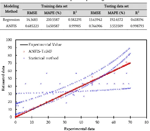
A comparison between ANFIS and the statistical model was made and the results are presented in Table 8 and Fig. 8. The comparison between ANFIS and least square regression methods through RMSE, MAPE, and R2 _{criteria shows that ANFIS is a more powerful method for} the estimation of xanthate decomposition percentage than the least square regression method. Furthermore, Fig. 8 clearly shows that the the estimation of xanthate decomposition percentage by ANFIS is

significantly more accurate than that of the regression method.

Table 7 Performance of ANFIS models with different number of input MFs in estimation of xanthate decomposition percentage

No. of input MFs

Training data set Testing data set RMSE MAPE (%) R2 _{RMSE MAPE (%) R}2

Fig.7 IF–THEN rules after training that can be used for the estimation of xanthate decomposition percentages at different solution conditions.

Table 8 The comparison between ANFIS model (Triangular MF and number of input MFs 9 9 9) with least squares regression model in the estimation of

xanthate decomposition percentage

Modeling Method

Training data set Testing data set

RMSE MAPE (%) R2 _{RMSE MAPE (%) R}2

Regression 14.3683 210.5587 0.582291 13.63942 192.4572 0.618196 ANFIS 0.685223 1.650587 0.99905 0.766906 3.553509 0.998793

Fig.8 The estimated xanthate decomposition percentage by ANFIS-TriMF and statistical methods vs. experimental data.

4.

Conclusion

In this research, the estimation of xanthate decomposition percentage was carried out based on the solution temperature, pH, and time through the least squares regression and ANFIS methods. The best subsets regression in the Minitab 17 package indicated that the model with all of the variables has the highest R2 _{(58%) and adjusted R}2 (57.9%), and the lowest Mallows' Cp value (4.0) and S value (14.402). The least squares regression through general regression by Minitab 17 proposed the following equation for the estimation of xanthate decomposition percentage:

Decomposition % = 0.24298 Temp – 26.1 pH – 0.205 Time + 0.0654 Temp×pH + 0.000692 Temp×Time + 0.000283 pH×Time

The validity of the model was confirmed through an analysis of the variance table and residual plots.

Different ANFIS models were constructed with various types and numbers of MF and the best results were obtained by Triangular MF and the number of input MFs 9 9 9. The low values of RMSE and MAPE (0.77 and 3.55%) for this model confirmed the ability of this model in

the estimation of xanthate decomposition percentage. The rule viewer GUI after training can be easily applied for the estimation of xanthate decomposition percentage at any point of temperature, pH, and time.

The comparison of ANFIS and the statistical method revealed that the ANFIS model is a more powerful method than the statistical method for the estimation of xanthate decomposition percentage.

REFERENCES

[1] Fuerstenau, M.C., Chander, S., Woods, R., 2007. Sulfide mineral flotation. In: Fuerstenau, M.C., Jameson, G., Yoon, R. H., (Eds.), Froth flotation a century of innovation. Society for Mining, Metallurgy, and Exploration, Inc. (SME), Littleton, Colorado, pp. 425-464.

[2] Bulatovic, S.M., 2007. Handbook of Flotation Reagents. 1st _ed. Elsevier, Amsterdam.

[3] Wang, D., 2016. Flotation reagents: Applied surface chemistry on minerals flotation and energy resources beneficiation, Springer, Singapore, pp. 9-38.

[4] Wills, B. A. and Napier-Munn, T., 2006. Wills' mineral processing technology: An introduction to the practical aspects of ore treatment and mineral recovery, 7th_{, Elsevier, Amsterdam, pp.} 267-352.

[5] NICNAS, 2000. Sodium Ethyl Xanthate: Priority Existing Chemical Secondary Notification Assessment, Australian Government Pub. Service, Australia, Canberra, Australia.

[6] Sun Z., Forsling, W., (1997). The degradation kinetics of ethyl-xanthate as a function of pH in aqueous solution. Minerals Engineering, 10 (4), 389-400.

[7] Trudgett, M., 2005. The ultra-trace level analysis of xanthates by high performance liquid chromatography, M.Sc. Thesis, University of Western Sydney, Australia.

[8] Molina, G. C., Cayo, C. H., Rodrigues, M. A. S., Bernardes, A. M., (2013). Sodium isopropyl xanthate degradation by advanced oxidation processes, Minerals Engineering, 45, 88–93. [9] Shen, Y., Nagaraj, D.R., Farinato, R., Somasundaran, P., (2016).

Study of xanthate decomposition in aqueous solutions, Minerals Engineering, 93, 10-15.

[10] Oliveira, C.R., Rubio, J., (2009). Isopropylxanthate ions uptake by modified natural zeolite and removal by dissolved air flotation, International Journal of Mineral Processing, 90, 21–26. [11] Mielczarski, J., (1986). The role of impurities of sphalerite in the

adsorption of ethyl xanthate and its flotation. International Journal of Mineral Processing, 16(3/4), 179−194.

[12] Silvester, E., Truccolo, D., Fu, P., (2002). Kinetics and mechanism of the oxidation of ethyl xanthate and ethyl thiocarbonate by hydrogen peroxide. Journalof theChemical Society,PerkinTransactions, 2, 2(9), 1562−1571.

[13] Fagadar-Cosma, G., Taranu, I., Fagadar-Cosma, E., (2003). Electrochemical oxidation of sodium ethyl xanthate in aqueous solutions. Revue Roumaine de Chimie, 48(2), 131−136. [14] Jin, X., Shui-yu, S., Ping, Z., He-shan, C., (2005). Degradation of

remainder xanthate in flotation wastewater by fenton reagent. Environmental Protection of Chemical Industry, 25(2), 125−127. [15] Deo, N., Natarajan, K. A., (1998). Biodegradation of some organic flotation reagents by bacillus polymyxa. Bioremediation Journal, 2(3), 205-214.

[16] Chockalingam, E., Subramanian, S., Natarajan, K.A., (2003). Studies on biodegradation of organic flotation collectors using Bacillus polymyxa, Hydrometallurgy, 71, 249–256.

[18] Mathur, N., Glesk, I., Buis, A., (2016). Comparison of adaptive neuro-fuzzy inference system (ANFIS) and Gaussian processes for machine learning (GPML) algorithms for the prediction of skin temperature in lower limb prostheses. Medical Engineering & Physics, 38(10), 1083–1089.

[19] Atia, D. M., El-madany, H. T., (2017). Analysis and design of greenhouse temperature control using adaptive neuro-fuzzy inference system, Journal of Electrical Systems and Information Technology, 4(1), 34-48.

[20] Mustafa, S., Hamid, A., Naeem, A., Sultana, Q., (2004). Effect of pH, temperature and time on the stability of potassium ethyl xanthate. Journalof theChemical SocietyofPakistan, 26(4), 363-366.

[21] Chen, X., Hu, Y., Peng, H., Cao, X., (2015). Degradation of ethyl xanthate in flotation residues by hydrogen peroxide. Journal of Central South University, 22, 495-501.

[22] Shen, Y., Nagaraj, D.R., Farinato, R., Somasundaran, P., (2016). Study of xanthate decomposition in aqueous solutions. Minerals Engineering, 93, 10–15.

[23] Iwasaki, I., Cooke, S.R.B., (1958). The Decomposition of Xanthate

in Acid Solution. Journal of the American Chemical Society, 80(2), 285-288.

[24] Esen, H., Inalli, M., Sengur, A., Esen, M., (2008). Modelling a ground-coupled heat pump system using adaptive neuro-fuzzy inference systems. International Journal of Refrigeration, 31, 65–74.

[25] Guney, K., Sarikaya, N., (2009). Comparison of adaptive-network-based fuzzy inference systems for bandwidth calculation of rectangular microstrip antennas. Expert Systems with Applications, 36, 3522–3535.

[26] Zounemat-Kermani, M., Teshnehlab, M., (2008). Using adaptive neuro-fuzzy inference system for hydrological time series prediction. Applied Soft Computing, 8, 928–936.

[27] Wang, Y.M., Elhag, T. M. S., (2008). An adaptive neuro-fuzzy inference system for bridge risk assessment. Expert Systems with Applications, 34, 3099–3106.

[28] Basics of best subsets regression (2016). Retrieved 7 March 2017, from http://support.minitab.com/en-us/minitab/17/topic-