www.geosci-model-dev.net/9/823/2016/ doi:10.5194/gmd-9-823-2016
© Author(s) 2016. CC Attribution 3.0 License.
CellLab-CTS 2015: continuous-time stochastic cellular automaton
modeling using Landlab
Gregory E. Tucker1,2, Daniel E. J. Hobley1,2, Eric Hutton3, Nicole M. Gasparini4, Erkan Istanbulluoglu5, Jordan M. Adams4, and Sai Siddartha Nudurupati5
1Cooperative Institute for Research in Environmental Sciences (CIRES), University of Colorado, Boulder, USA 2Department of Geological Sciences, University of Colorado, Boulder, USA
3Community Surface Dynamics Modeling System (CSDMS), University of Colorado, Boulder, USA 4Department of Earth and Environmental Sciences, Tulane University, New Orleans, USA
5Department of Civil and Environmental Engineering, University of Washington, Seattle, USA Correspondence to: Gregory E. Tucker ([email protected])
Received: 11 September 2015 – Published in Geosci. Model Dev. Discuss.: 2 November 2015 Revised: 31 January 2016 – Accepted: 10 February 2016 – Published: 29 February 2016
Abstract. CellLab-CTS 2015 is a Python-language soft-ware library for creating two-dimensional, continuous-time stochastic (CTS) cellular automaton models. The model do-main consists of a set of grid nodes, with each node assigned an integer state code that represents its condition or composi-tion. Adjacent pairs of nodes may undergo transitions to dif-ferent states, according to a user-defined average transition rate. A model is created by writing a Python code that de-fines the possible states, the transitions, and the rates of those transitions. The code instantiates, initializes, and runs one of four object classes that represent different types of CTS mod-els. CellLab-CTS provides the option of using either square or hexagonal grid cells. The software provides the ability to treat particular grid-node states as moving particles, and to track their position over time. Grid nodes may also be as-signed user-defined properties, which the user can update af-ter each transition through the use of a callback function. As a component of the Landlab modeling framework, CellLab-CTS models take advantage of a suite of Landlab’s tools and capabilities, such as support for standardized input and out-put.
1 Introduction
The discovery of cellular automata in the 1940s (Von Neu-mann, 1951) laid the groundwork for a type of computa-tional model that distinctly differs from numerical solutions
2014), and permafrost features (Kessler et al., 2001; Plug and Werner, 2002).
One interesting variant on CA is the continuous-time stochastic CA, in which cell transitions occur at randomly chosen time intervals rather than in discrete steps. These models are especially attractive for geoscience applications because their parameters represent rates that can be di-rectly related to field and laboratory measurements, and be-cause they avoid the need for a discrete-time approximation (Narteau et al., 2001, 2009; Rozier and Narteau, 2014). For example, once appropriate length and timescales have been chosen, the cell-transition rules take on meaningful dimen-sions and can be compared to an average propagation rate of a reaction front, the average frequency and depth of soil dis-turbance by burrowing organisms, or any other quantity of interest that has a definable rate.
Here we describe a new modeling framework called CellLab-CTS, which is written in Python and built on the Landlab platform (Landlab Development Team, 2016). CellLab-CTS allows one to quickly build and explore two-dimensional, continuous-time stochastic CA models. A novel feature is the option of using either square or hexagonal cells. The aim of CellLab-CTS is to greatly simplify the process of creating, configuring, and exploring 2-D CA models. We provide a brief background on the theoretical framework, de-scribe the algorithms and data structures used to implement CellLab-CTS, and present several examples that illustrate its versatility.
2 Background
Wolfram (1983) defines cellular automata as “simple math-ematical idealizations of natural systems [that] consist of a lattice of discrete identical sites, each site taking on a fi-nite set of...values.” Like other types of mathematical model, CA models describe natural systems in the form of symbolic logic (Chopard and Droz, 1998). They are similar to partial differential equations in the sense that both can be written in compact form; in the case of a CA, however, the compact form is a set of algorithms (rules) that evolve the numerical value of cell states or change cell attributes based on interac-tions among cells. In both cases, the compact form itself (the equation or the algorithm) often reveals little about the dy-namics of the system and its potential spatial outcomes and self-organization. To discover and visualize the system’s be-havior, one needs to perform numerical calculations. These calculations are often more computationally efficient, involv-ing fewer parameters or degrees of freedom, than in the case of numerical solutions of comparable PDEs. The need for numerical calculations applies especially for complex phys-ical systems that are computationally irreducible, such that the physical state of the system at a certain time can only be predicted by simulating the evolution of states through time.
In a classical CA, the cell values evolve over a sequence of discrete time steps on the basis of a set of deterministic rules that describe the nature of the system (e.g., Chopard and Droz, 1998). These rules describe sequential transitions in the state of each cell as a function of the other cells in its immediate neighborhood. Since cellular automata were first invented in the late 1940s, many variations on this ba-sic concept have been developed and explored. For example, some use continuous (real) numbers instead of discrete lat-tice states (as in the example of latlat-tice Boltzmann models; e.g., Chen and Doolen, 1998). The class of stochastic cellular automata use random rather than deterministic rules for up-dating, which allows one to explore ensembles of outcomes. Of particular interest here are continuous-time stochas-tic (CTS) cellular automaton models: those in which tran-sitions between discrete cell states occur at random time in-tervals. This technique was introduced into the geosciences by Narteau et al. (2001) in an application to the dynamics of the core-mantle boundary. The same approach was later used (in 3-D instead of 2-D) to study the growth of instabil-ities that leads to the formation of eolian bedforms (Narteau et al., 2009). In the next section, we describe the theory be-hind the CTS approach; the following sections describe how the concept is implemented in CellLab-CTS.
3 Cellular automata with stochastic, pairwise transitions
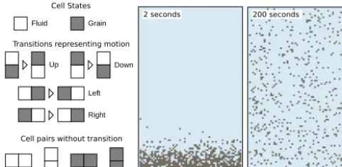
CellLab-CTS implements a two-dimensional, continuous-time stochastic cellular automaton with pairwise transitions (Narteau et al., 2001). As a simple example, consider a model for the mixing of suspended-sediment particles in a turbulent fluid with isotropic turbulence. As in a classical CA, the do-main of interest is represented as a lattice of cells, each of which belongs to one ofNdiscrete states. For suspended sed-iment, we have two states: a cell may be occupied by fluid, or by a sediment grain. The width of each cell is taken to be the characteristic diameter of a sediment grain. The lattice repre-sents a vertical cross section through the fluid. Such a model might be initialized with a bed of sediment particles below a body of (initially) still fluid (Fig. 1).
Cell States
Fluid Grain
Transitions representing motion
Up Down
Left Right
Cell pairs without transition
2 seconds 200 seconds
Figure 1. CellLab-CTS model of grains suspended in a stirred (tur-bulent) fluid. Left: illustration of cell states, cell-pair states, and cell-pair transitions. Grains are assumed to be neutrally buoyant, and turbulence is isotropic, so that there is an equal probability of grain motion in each direction. Grain motion is modeled as a transi-tion that switches the positransi-tion of grain and fluid at a user-specified rate. In this example, we assume that the grains are 1 mm diame-ter tea leaves and the characdiame-teristic turbulent velocity fluctuation is 0.01 m s−1, so that cell sizeδ=0.001 m and the mean transition rate is 10 cells s−1.
p(τ ) =RTexp(−RTτ ) , (1)
whereτ is the time between transitions at a particular pair, andRT is the average transition rate for a particular transition
type (with dimensions of 1/T). The reciprocal of the tran-sition rate,τ¯=1/RT, is the average waiting time between
transitions of that type. Once the cell size,δ, is specified, one obtains a mean transition velocity:VT=δ/τ¯.
The transition probability or rate depends on the states of the two cells. We will refer to a particular pairing of cell types as the pair state. The number of pair states depends on the number of cell states, and on whether spatial orienta-tion matters. For example, if our turbulence is isotropic and the particles are neutrally buoyant, the transition probability for a fluid-plus-particle pair would be independent of orien-tation. In that case, there are N (N+1)/2=3 unique pair states: fluid–fluid, fluid–grain, and grain–grain (Fig. 1). On the other hand, if the particles are denser than the fluid, ori-entation matters because the downward transition rate will be greater than the upward or lateral rates (Fig. 2). When di-rection matters, we have MN2 cell-pair states, whereM is the number of orientations: two for a raster grid (vertical and horizontal), and three for a trigonal lattice with hexagonal cells. In the suspended-sediment example,N=2; a square grid impliesM=2, so that there are eight cell-pair states (the six shown in Fig. 2 plus fluid-fluid and grain-grain pairs).
Note that it is possible, and often likely, to have a partic-ular node (representing, say, a grain) scheduled to undergo more than one transition. For example, consider a “grain” node in the suspended-sediment model. That node belongs to four different pairs. If the grain is surrounded by fluid nodes, then each of those pairs will have the potential to undergo a
200 seconds Horizontal motion
Rh = u'δ
= 10 cells/s
Downward motion
Rd = Rh + w/2δ
= 10.55 cells/s
Upward motion
Ru = Rh - w/2δ
= 9.45 cells/s
Figure 2. Turbulent suspension model with grains (1 mm tea leaves) that are 0.2 % denser than the surrounding fluid. Left: illustration of cell-pair transitions representing motion in the four directions. Grain settling velocity of 0.0011 m s−1imparts asymmetry to the transition probabilities.
transition in which the grain and fluid switch places. When such a transition occurs at one of the four pairs, it invalidates the other three pair transitions. Below, we explain how this common situation is handled.
The suspended-sediment model illustrates the advantage of a stochastic as opposed to deterministic approach; we are dealing with a system that is in fact inherently stochastic and unpredictable, because the grain motions arise from turbu-lent velocity fluctuations. It is of interest to know how the in-herent variability leads to emergent pattern formation, such as the diffusion-like time evolution of average concentration (without settling) or the emergence of a Rouse-like concen-tration profile (with settling).
The suspended-sediment examples also illustrate how it is possible to scale a CTS model. Here, we have chosen the cell size as the diameter of the particles (1 mm), and the timescale as 1 s. For the neutrally buoyant case, the transi-tion rate is set to equal a characteristic velocity perturbatransi-tion of 1 cm s−1= 10 cells s−1. For the denser-than-fluid case, the transition probabilities for upward and downward motion are decreased or increased, respectively, by a factor of=w/2δ, wherew=0.0011 m s−1is settling velocity andδ=0.001 m is cell width. Thus, the scales and transition rates are not arbitrary but have a direct physical meaning. For more on this point, see Narteau et al. (2009) and Rozier and Narteau (2014).
4 Algorithms, implementation, and capabilities
CellLab-(a) Raster grid (b) Hex grid
Cell
Node Link
Figure 3. Schematic illustration of CellLab-CTS grid types and ge-ometric primitives. (a) Regular (raster). (b) Trigonal lattice with hexagonal cells. Note that standard link orientation is within the
x≥yhalf plane; in other words, the angle of a link,θ, with respect to the positivexaxis is always−45◦≤θ≤135◦.
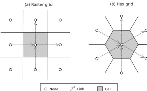
CTS can use either of the two grid types that are commonly used in cellular automata: a raster grid with square cells, or a trigonal grid with hexagonal cells (Fig. 3). Landlab’s grid design lends itself naturally to pairwise cellular automata be-cause the data structures include links: directed line segments that represent the connections between adjacent cell pairs. 4.1 Landlab’s grid design
One of Landlab’s unique features is the ability to create any of a variety of grid types, including raster (square cells), rectilinear (rectangular cells), trigonal (hexagonal cells), Delaunay–Voronoi (Voronoi polygon cells), and radial (a special class of Delaunay–Voronoi in which nodes are ar-ranged in concentric circles). Each grid type uses the same flat data structure, in which grid elements are listed se-quentially in one-dimensional arrays. For CellLab-CTS, this means that one can implement CA models using either a raster or hexagonal grid.
To understand how CellLab-CTS works, it is helpful to know a bit about Landlab’s grid composition and data struc-tures. Each grid contains a set of nodes, which are points in(x, y)space (Fig. 3). Each adjacent pair of nodes is con-nected by a link, which is an oriented line segment. Every link connects a tail node to a head node, with the implied di-rection being from the tail to the head. Each node in the grid interior – that is, every node except those along the perime-ter of the grid – sits inside a polygon known as a cell. In the case of CellLab-CTS, cells are either squares or hexagons. Every cell face is crossed by a link. (Note that CellLab-CTS actually operates on arrays of nodes rather than cells, so that the outer perimeter of cell-less nodes may be included as a boundary condition; for this reason, the internal documenta-tion refers to nodes and node pairs rather than cells and cell pairs.)
Cell
Node (core) Active Link Face
Inactive Link Node (open boundary)
Node (closed boundary)
Figure 4. Example of a simple Landlab raster grid, illustrating open- and closed-boundary nodes, and active and inactive links.
To facilitate boundary-condition handling, nodes come in two flavors: core nodes and boundary nodes (Fig. 4). Core nodes are those that constitute the computational domain. When a Landlab grid is created, the default configuration has all interior nodes flagged as core nodes, and all perimeter nodes flagged as boundary nodes. For modeling irregular do-mains (such as a watershed within a rectangular DEM), one can set up a grid to have boundary nodes in the interior as well as along the perimeter.
4.2 Node and node-pair (link) states
In order to implement a cellular automaton model, CellLab-CTS assigns an integer node state to each node in the grid. These values are encoded in a one-dimensional array of inte-gers called the node-state grid. The number of possible node states and their transition behaviors are determined by the model developer, as explained below. For example, in the ex-ample of turbulent suspension (Figs. 1 and 2), there are two possible node states: 0 and 1, representing fluid and a solid particle, respectively.
As discussed above, a CellLab-CTS model is based on transitions from one pair of node states to another pair. Each unique pair is referred to as a pair state or a link state. To im-plement pairwise transitions, CellLab-CTS takes advantage of the fact that a Landlab grid includes a set of links con-necting pairs of neighboring nodes. We can exploit this fact by creating a data structure in which each active link in the grid is assigned a pair code. The pair code is a single integer value that represents the states of the two adjacent nodes, and possibly also the spatial orientation of the pair.
To understand how pair coding works, we need to look more closely at orientation. In some applications, spatial ori-entation does not matter. For example, in the isotropic sus-pension model (Fig. 1), the transition rate for a solid-grain pair is the same regardless of whether the pair in question is horizontal (aligned with thex axis) or vertical (aligned with theyaxis). In other applications, orientation does matter. For example, when gravitational settling is added to the turbulent suspension model, the transition rates differ for horizontal and vertical pairs (Fig. 2). Moreover, the transition rate for a vertical pair also depends on whether the solid particle lies above the fluid particle, or vice versa.
To accommodate these difference, CellLab-CTS allows users to create either an oriented or a non-oriented model. In a non-oriented model, the sequence of node-state codes associated with the nodes of a given link, say 0 at the link’s tail node and 1 at its head node, is treated the same regardless of whether the link is vertical, horizontal, or (in the case of a hex grid) at an angle of+30◦or−30◦. For a non-oriented model, whether raster or hex, there areN2unique link states, whereNis the number of possible node states. For example, the isotropic turbulent suspension model (Fig. 1), which is an example of a non-oriented (raster) model, there are just four link states: (1) two adjacent fluid cells, (2) fluid cell at the link’s tail and a solid cell at the link’s head, (3) a solid cell at the link’s tail and a fluid cell at its head, and (4) two adjacent solid particles. Note that the order from tail node to head node still matters; the pair 0→1 is different from the pair 1→0.
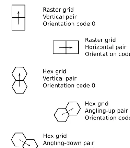
By contrast, an oriented model treats cell pairs in differ-ent oridiffer-entations as differdiffer-ent pair states. In a raster grid, there are two possible orientations: horizontal and vertical. In a hex grid, there are three. In our examples, these three hex-grid orientations are vertical, angling up (+30◦), and angling
Raster grid Vertical pair Orientation code 0
Raster grid Horizontal pair Orientation code 1
Hex grid Vertical pair Orientation code 0
Hex grid Angling-up pair Orientation code 1
Hex grid
Angling-down pair Orientation code 2
Figure 5. Illustration of cell-pair orientations and corresponding orientation codes. Arrows represent links, each of which connects a tail node to a head node.
down (−30◦) (Fig. 5; note that one can rotate this so that one of the axes is horizontal rather than vertical, but in either case there are still three orientations). Each of these is given a sep-arate pair-state code, indicating that the transition type and rate may be different depending on orientation. For exam-ple, in an oriented raster, the pair 0→1 has different codes for horizontal and vertical orientation. An oriented raster has 2N2link states, whereas an oriented hex has 3N2link states. 4.3 Transitions and the event queue
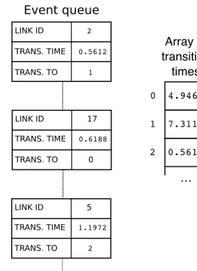
Unlike a traditional discrete-time CA, CellLab-CTS does not use time steps. Instead, we iterate through a sequence of pair transitions, or events. As noted earlier, each pairwise transi-tion is associated with a time-independent statransi-tionary Poisson process. Thus, the time intervals between successive transi-tion events at a particular locatransi-tion are stochastic, with an ex-ponential probability distribution (Eq. 1). At the start of a run, every node pair (i.e., every link) is assigned a transition time. These transition-event times are generated at random from an exponential probability distribution, the mean of which isτ¯i= 1/RT i, whereiindicates the particular type of
Once the initial event times are assigned, we need to iterate through them in chronological order. In order to place events in the correct time sequence, we adopt an approach that is commonly used in other types of discrete-event simulations (e.g., Karimabadi et al., 2005; Omelchenko and Karimabadi, 2006, 2007), in which future events are recorded in a queue that sorts them according to time of occurrence. When a new event needs to be scheduled, we create an event object, which stores the location of the transition, the time at which it is scheduled to occur, and the new node states. This event ob-ject is then placed in the event queue: a data structure that contains all scheduled future transitions (Fig. 6). The event queue is implemented as a heap, using the Python heapq library. Events in the event queue are automatically and effi-ciently sorted such that the event with the smallest value of transition time – that is, the next one to occur – is always at the top. At the same time, we also record the transition time in a separate array that contains the transition times for every link (Fig. 6). Recording the transition times in two differ-ent locations allows us to handle the common case in which a scheduled transition becomes invalid because the state of one or both cells has changed. The easiest way to understand how this works is to examine the algorithm for implementing pair transitions, which we turn to next.
4.4 Algorithm for pair transitions
At the beginning of a CellLab-CTS simulation, we set up the initial array of node states. We then loop over all active links, assigning to each one the corresponding pair code. The pair code,Li, for a given linkiis calculated from the state of each
node and the link’s orientation:
Li=OiN2+TiN+Hi, (2)
whereOiis the link’s orientation code (Fig. 5),Ti is the state
of the tail node,Histate of the head node, andNis the
num-ber of potential node states in the model. Recall that a partic-ular pair state may have zero, one, or more than one possible transition. For those pair states that have only one possible transition, the transition time is selected at random from an exponential distribution with the appropriate rate parameter, and an event object is created and pushed to the event queue. When a given pair state is associated with two or more possi-ble transitions, transition times drawn at random number for each of the potential transitions. The soonest of these is then entered into an event object and pushed to the event queue.
A scheduled event at one pair can become obsolete if one or both nodes changes state as a result of a transition in an-other pair to which the node is connected. For instance, con-sider a particle (state 1) surrounded by four fluid nodes (state 0) in the suspended-sediment example. The particle belongs to four different pairs: it is connected to the nodes above, below, right, and left. Each of these pairs will have a tran-sition scheduled in which the solid and fluid states switch places, simulating motion of the grain. When a transition
oc-LINK ID 2
TRANS. TIME 0.5612
TRANS. TO 1
Event queue
Array of
transition
times
LINK ID 17
TRANS. TIME 0.6188
TRANS. TO 0
LINK ID 5
TRANS. TIME 1.1972
TRANS. TO 2
...
...
0 4.9462
1 7.3115
2 0.5612
Figure 6. Illustration of the event queue and the transition-time ar-ray (next_update). Each event object contains the ID number of the link, the time at which the next transition is scheduled to oc-cur, and the link-state code for the transition (that is, the code for the new cell pair after transition occurs). Left: events are stored in a heap that is sorted by transition time, soonest on top. Right: the transition-time array, which is simply an ordered array, indexed by link ID, containing the time of the next scheduled transition at the corresponding link. If the transition time for an event object does not match the corresponding entry in the transition-time array, it means that the originally scheduled transition has been nullified by other transitions and is no longer valid (see text).
curs at one of the four pairs, the other three scheduled transi-tions immediately become invalid, and their scheduled tran-sitions should be ignored when they are popped from the event queue. To handle this situation, whenever an event is scheduled, its transition time is also recorded separately in the transition-time array (as is done in the discrete-event al-gorithms of Karimabadi et al., 2005 and Omelchenko and Karimabadi, 2006, 2007). Then, each time an event is popped from the event queue, it is executed only if its transition time matches the entry in the transition-time array.
The event-loop algorithm is illustrated in Algorithm 1. Note that each event objectEincludes a time of occurrence (E.time), the ID number of the link at which the event occurs (E.link), and the new link state to which the pair transitions (E.xn_to).
transi-Algorithm 1 Event loop Tr←duration for run
t←0
whilet < Trand event queue is not empty do
E←pop next event from event queue
ifE.time matches the event time for this link recorded in the transition-time array then
Process the transition event, schedule the next event, and update surrounding pairs
end if
t←E.time end while
tions at the affected node(s). Therefore, the pair-state codes for each pair attached to the transitioning nodes must be up-dated, and new events generated and scheduled.
Algorithm 2 Processing a transition event
Update the states of the two nodes attached to the link Update the link’s pair code
Generate the next event for this link (if any) and push it to the event queue
forN=each of the link’s two nodes (tail and head) do if the state ofNhas changed as a result of this transition then
for all other active linksLconnected toNdo Update the state-code forL
Generate the next event forLand push it to the event queue
Update the entry forLin the transition-time array end for
end if end for
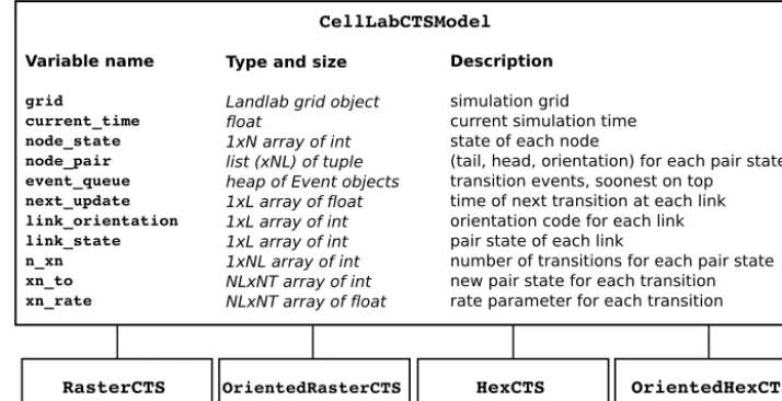
4.5 Class hierarchy and data structures
CellLab-CTS uses Python classes to implement four sub-types of the CA model. The class inheritance structure is quite simple (Fig. 7). The base class, CellLabCTSModel, handles most of the primary data structures. The simulation grid is represented using a Landlab ModelGrid object (either a RasterModelGrid or HexModelGrid). Thenode_state array contains the state-code for every node (recall that Land-lab nodes represent cells in the model; LandLand-lab reserves the term cell for polygons that surround interior nodes).
Information about the relationship between link states and node states is contained in the node_pair list. When a transition occurs, this list is used to look up the new states of the two nodes given the new state of the link. The list is indexed by the pair-state codes, and each entry is a three-element tuple: (T , H, O), where T is the state of the tail node,His the state of the head node, andOis the orientation of the link. For example, the configuration represented by pair-state number three would be found atnode_pair[3].
As discussed previously, transition events are recorded in a heap known as the event queue. The time of transition for each pair (link) is also recorded in thenext_updatearray (Fig. 6).
For models in which pair orientation matters, we need to keep track of the orientation code for each pair. This is done usinglink_orientation, an array of integer orientation codes (as defined in Fig. 5), whose length is equal to the num-ber of links in the grid. The state of each pair is encoded in thelink_statearray. Finally, information about pair-state transitions is encoded in three arrays. We encode the number of potential transitions for each pair state in the array n_xn. For every transition type, we need to record the new pair state and the rate; these two pieces of information are recorded in xn_toandxn_rate, respectively. Both are two-dimensional arrays with dimensions equal to the number of unique pair states and the maximum number of transitions for any given pair state.
4.6 Tracking properties associated with moving particles
The suspended-particle simulations (Figs. 1 and 2) are exam-ples of models in which certain node states represent moving particles. For such models, it is often desirable to keep track of various properties associated with these particles. For ex-ample, one might wish to keep track of the original position of a particle, or calculate a position-dependent accumulation or loss of a property such as cosmogenic nuclide concentra-tion, luminescence, or chemical composition. CellLab-CTS provides the ability to define and track user-defined data that are associated with certain node states, which are treated as mobile particles.
To implement property tracking, the user defines an ar-ray or list of properties that are assigned to nodes in their initial locations. The properties themselves may be of any data type; for example, for a simple scalar property, one might use floats, whereas for a collection of properties, user-defined objects containing multiple data items could be as-signed. CellLab-CTS then creates an array that contains, for each node, the index in the user-defined property array/list that corresponds to that node. To handle movement of par-ticles, each transition includes a flag indicating whether the transition in question involves an exchange of properties be-tween the two nodes in the pair. For example, the transitions in the turbulent suspension model (Figs. 1, 2) represent par-ticle motion, and would therefore be flagged as involving an exchange of properties between the node pairs.
Variable name
grid
current_time node_state node_pair event_queue next_update link_orientation link_state
n_xn xn_to xn_rate
Description
simulation grid current simulation time state of each node
(tail, head, orientation) for each pair state transition events, soonest on top
time of next transition at each link orientation code for each link pair state of each link
number of transitions for each pair state new pair state for each transition rate parameter for each transition Type and size
Landlab grid object float
1xN array of int list (xNL) of tuple heap of Event objects 1xL array of float 1xL array of int 1xL array of int 1xNL array of int NLxNT array of int NLxNT array of float
CellLabCTSModel
RasterCTS OrientedRasterCTS HexCTS OrientedHexCTS
Figure 7. CellLab-CTS class hierarchy and main data structures. The base class, CellLabCTSModel, has four subclasses: RasterCTS, Ori-entedRasterCTS, HexCTS, and OrientedHexCTS. A user selects one of these four subclasses based on whether the model to be built has a hex or raster grid, and on whether pair orientation matters.Nis number of grid nodes,Lis number of grid links,N Lis number of possible link (node pair) states, andN T is maximum number of transitions for any link state.
example, suppose that property data for node 5 are stored at array location 19. This would indicate that the particle repre-sented by node 5 began at node 19 and subsequently moved to node 5.
Updating of properties is handled by the CellLab-CTS user, and it involves the use of a callback function. If a par-ticular transition type involves particle motion, and one or more user-defined properties of particles evolves in time, the user would write a function to update these properties. The function arguments are a CellLabCTSModel object (i.e., the instance of one of the four subclasses listed in Fig. 7), the IDs of the two nodes involved in the transition, and the time at which the transition occurs. This function is then passed as an optional argument when the transition in question is set up at the beginning of a run. Then, whenever a transition of that type takes place, CellLab-CTS automatically calls the user’s function. This use of a callback function gives the user flexi-bility to implement any kind of updating of properties during each transition event.
As an example of user-defined property updating, imagine a version of the suspended-sediment model (Fig. 2) in which the grains are quartz sand (instead of tea leaves), and pos-sess the property of luminescence. When quartz grains are exposed to background ionizing radiation in the soil, elec-trons gradually become displaced from their rest states, and become trapped within defects in the crystal lattice. When the grain is exposed to light, the trapped electrons are re-leased, returning to their rest states and giving off a faint glow in the process. This phenomenon, known as optically stimulated luminescence (OSL), is commonly used in geo-logic dating applications (Rhodes, 2011).
Imagine then that our grains begin with a certain lumines-cence signalL, which we will assume is initially uniform for all grains. Imagine also that a light is positioned above the container, but that the fluid is partly opaque, so that the light intensity attenuates with depth below the surface. For quartz OSL, the rate of signal loss (bleaching) can be approximated by
dL dt = −
L
T (z), (3)
wheretis time andT (z)is an effective timescale for bleach-ing that depends on the incombleach-ing photon flux and a material-dependent bleachability parameter (both integrated over the light spectrum). Because the photon flux attenuates with depth in the fluid column,z, according to the Beer–Lambert law, the bleaching timescale grows with depth below the fluid surface:
T (z)=T0exp(z/z∗) , (4)
wherez∗ is the attenuation length scale, which depends on
the fluid opacity (note that we ignore scattering here). For our example, we will useT0= 2.42 s (Bailey and Arnold, 2006) andz∗=0.025 m. The latter represents quite opaque fluid
(think tea with milk), and is used here simply to create a strong (∼50×) variation in bleaching rate through the depth of our 10 cm container. Grains that diffuse toward the top of the container will therefore experience a much higher bleach-ing rate than those that settle toward the bottom.
Fra
ction of initia
l luminesc
ence
signa
l
0 1
FLUID
GRAINS
Figure 8. Model of turbulent sediment suspension, showing the computed luminescence signal after 20 s of stirring and bleaching. The original luminescence signal is removed (bleached) by expo-sure to light. Because light intensity declines exponentially from top to bottom, grains near the bottom are less fully bleached than those near the top. Turbulent mixing disperses the partially bleached grains.
either or both nodes represents a particle. If so, the corre-sponding entry in the user’s luminescence array is updated by extrapolating Eqs. (3) and (4):
Li←Liexp
− t−tl
T0ez/z∗
, (5)
wheret is the current time andtl is the last time the
lumi-nescence at nodeiwas updated (which the callback function also tracks). The turbulent suspension model with bleaching is illustrated in Fig. 8. As one might expect, the rapid attenua-tion of light creates a strong vertical gradient in the degree of bleaching, with some dispersion that reflects turbulent mix-ing. Although this particular example is somewhat unrealistic in that light attenuation is treated as independent of sediment concentration (in other words, light passes equally through fluid and grains), the example illustrates the ability to treat certain cell states as moving particles, to track their move-ment, and to associate each particle with one or more prop-erties.
5 Other examples
Three additional examples serve to illustrate the diversity of applications that can be written using CellLab-CTS. These applications span the fields of geomorphology (chemical weathering of crystalline rock), epidemiology (a susceptible– infectious–recovered model of disease spread), and granular mechanics (a lattice-grain model).
5.1 Weathering of fractured rocks
One of the current frontiers in geomorphology and soil sci-ence lies in understanding the transformation of rock to soil. One-dimensional reactive transport models have been used to study the time evolution of a weathering front in homo-geneous, unfractured rock (e.g., Lebedeva et al., 2007, 2010; Maher, 2010). In crystalline rocks, however, it is often ob-served that chemical alteration of the original rock takes place primarily along fracture planes, which serve as con-duits for water, oxygen, and reactive aqueous elements such as hydrogen ions (Pandey and Rajaram, 2014). The model shown in Fig. 9 implements a simple hypothesis for the trans-formation of parent rock into saprolite (material that has been chemically altered by not disaggregated). Nodes in the model represent mineral grains; a typical diameter of such grains in nature might be∼3 mm. The model begins with a network of fractures, each initially one grain wide. The rules repre-senting hydrology and geochemistry are deliberately simpli-fied for the sake of illustrating a single-transition CellLab-CTS model: any rock–saprolite pair has a fixed probability per unit time of transforming into a saprolite–saprolite pair. This example uses the RasterCTS class.
The model domain forms a set of fracture-bounded blocks of rock, which weather inward over time from their perime-ters. The effective probability of weathering of a grain de-pends on its local geometry: a grain exposed on only one side has a lower probability of weathering within a given time pe-riod than one exposed on all four sides, simply because of the combined probabilities in the latter. This simple geomet-ric principle leads to a gradual rounding of the blocks as they weather.
chemi-Figure 9. Three time slices from a CellLab-CTS model of bedrock weathering along fracture planes. Light-colored cells are unweathered mineral grains; dark-colored cells are grains that have been chemically altered to form saprolite (rock material that has been weathered but not displaced). Left to right: time 0, time 10, and time 30. Here the time is normalized by initial fracture width and weathering rate; one time unit represents the average time to weather fresh rock to a depth of one initial fracture width. For example, if fracture width (cell size) were 1 cm and weathering rate 10−5m yr−1, then one time unit=1000 years.
cally saturated and unsaturated fluid states (cf. Narteau et al., 2001). An interesting future challenge would be to couple a dissolution-crystallization model with a model of aqueous flow in the fracture network.
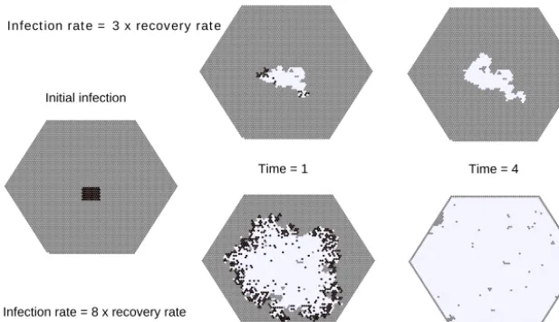
5.2 Susceptible–infectious–recovered model
The susceptible–infectious–recovered (SIR) concept is a classic mathematical model in epidemiology. The simplest form of the SIR model represents a population as having three compartments: those which are infected, those which have not yet been infected and are therefore susceptible to the disease, and those which have recovered and are now immune (Hethcote, 2000). Figure 10 illustrates an imple-mentation of the SIR model as a continuous-time stochastic cellular automaton, using a hex grid. Each node has one of three states: susceptible (gray), infectious (black), and recov-ered (white). Infection and recovery are modeled as stochas-tic processes. An infected node has a user-specified transi-tion rate to recovery (probability per unit time of recovering), which translates into an exponential probability distribution of recovery times with mean τ¯r (Eq. 1). When a
suscepti-ble node lies adjacent to an infectious node, there is a speci-fied infection rate (probability per unit time that the suscep-tible node will become infected). Again, this translates into an exponential probability distribution of time to infection, with meanτ¯I. Thus, for any adjacent susceptible–infectious
pair, there is a race against time: will the infected node re-cover before passing on the infection to its neighbor? The outcome depends on the ratio of infection to recovery rates. When the ratio is modest, an initial disease cluster spreads relatively slowly, and is likely to die out before spreading very far (Fig. 10, top row). When the ratio is higher, disease is likely to spread throughout the population, leaving few in-dividuals untouched (Fig. 10, bottom row).
Table 1. States in the CTS lattice gas and lattice-grain models.
State code Description
0 empty or fluid 1 moving upward
2 moving right and upward 3 moving right and downward 4 moving downward
5 moving left and downward 6 moving left and upward 7 resting
8 wall
5.3 Lattice-grain model
Initial infection
Infection rate = 8 x recovery rate
Time = 1 Time = 4
Infect ionrat e= 3xrecoveryrat e
Figure 10. A susceptible–infectious–recovered (SIR) model built with CellLab-CTS. This example compares runs with two different infec-tion rates (top and bottom rows, respectively). Gray is susceptible, black is infectious, and white is recovered. One time unit is one average recovery time. This example model uses the HexCTS subclass (non-oriented model with hexagonal cells).
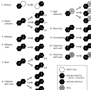
common for lattice-gas models), there are therefore six pos-sible directions. In addition, some models also include sta-tionary particles. Each iteration of a lattice-gas model has two steps: a movement step, in which each particle moves one unit in its given direction, and a collision step, in which collisions between particles are resolved by changing parti-cle directions (as a representation of collision and rebound between perfectly elastic particles).
A typical lattice-grain model starts with these basic rules but with modifications. Each cell may be occupied by only one grain (as opposed to one for each possible direction in lattice-gas models). Because grains are not perfectly elastic, collisions may result in a loss of momentum, with a speci-fied probability. Finally, gravity is represented by applying a certain probability for a particle to alter its direction and/or velocity (for those models that allow varying velocity among particles).
The stochastic, pairwise transition model of CellLab-CTS can be used to construct versions of both a lattice-gas and a lattice-grain model; the latter is simply a version of the for-mer that adds rules for gravity and friction. Here we present examples of both types of models. The examples are imple-mented on a hex grid with a vertical axis and two other axes at 60◦from vertical. There are nine possible node states,
cor-responding to the six directions of motion, an empty state, a resting state, and a wall state (Table 1).
The motion and collision rules for a pairwise CTS lattice gas model are illustrated in Fig. 11 and listed in Table 2. Be-cause the model is stochastic, with binary transitions, the rule set is somewhat different from that of a traditional determin-istic lattice-gas model (e.g., Chopard and Droz, 1998). There is no need to deal with three-way collisions, for example, and we allow only one particle to occupy each node. Fur-thermore, the stochastic nature of transitions means that
par-ticles effectively have varying velocity and momentum. This in turn raises the possibility of collisions from the side or be-hind (relative to a grain’s direction of motion), as one particle overtakes another. Such collisions are not possible in a tradi-tional lattice gas, in which particles have the same velocity and cannot overtake one another. Motion is implemented as a simple exchange of states (Fig. 11, top). In some cases, a collision may produce any of two or three different outcomes, as in the example of a head-on collision. In these cases, mul-tiple transitions are encoded, each with a reduced transition rate; this is equivalent to assigning a fractional probability to each of the potential outcomes. Interestingly, indirect col-lisions tend to be less common than head-on colcol-lisions, be-cause they only occur if one of the two particles does not move out of the way first.
The behavior of the CTS lattice-gas model is illustrated in Fig. 12, which shows particles in closed vessel. The num-ber of particles in each motion state remains roughly con-stant over time, indicating that momentum is conserved. The CTS lattice-gas model lacks the speed advantage of tradi-tional lattice-gas models; we present it here because it forms the basis for a cellular model of granular mechanics, which we turn to next.
1. Motion
3. Oblique 2. Direct collision
1/3
1/3 1/3
1/3
1/3 1/3
1/4
1/4 4. Oblique
rear
5. Rear
6. Collision with rest
7. Wall rebound
8. Glancing
9. Converging
10. Glancing with rest
11. Glancing with wall
EMPTY CELL
MOVING PARTICLE (arrow = direction)
RESTING PARTICLE
WALL
Figure 11. Motion and collision rules for a pairwise CTS lattice gas model. For states that have multiple transitions, the transition rate for each is reduced from unity to the fraction shown. Reduction to a one-fourth rate (instead of one-half) for rear collisions accounts for the possibility that the lead particle is faster (so no collision occurs).
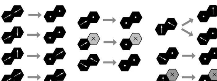
restitution. The corresponding frictional transitions are as-signed a rate off =1−e(except for rule 8, in which each of two frictional transitions is assigned a rate off/2; Fig. 13, upper right). This approach to inelastic collisions is similar, for example, to that of Károlyi and Kertész (1998).
Gravity is implemented by assigning transitions that have the effect of adding downward momentum (Fig. 14). Thus, upward-moving particles transition to resting ones, while resting ones transition to downward-moving particles, and so on. Each of these transitions is assigned a user-specified rate g. This parameter sets the timescale for the model; 1/g is intended to represent the time required for an initially sta-tionary grain to fall a distance of one cell. Because of the limitations of the CTS approach, these rules provide only an approximate representation of gravitational behavior. For ex-ample, in the CTS framework, the average speed (and hence momentum magnitude) of a particle reflects its average tran-sition rate. Because the trantran-sition rate parameter is constant for each transition type, it is not possible to represent accel-eration (though this limitation could be overcome in a future version by allowing a variable transition rate). For example, we approximate the tendency for velocity vectors to orient downward by applying the transitions shown in the third row
of Fig. 14, in which a particle moving both horizontally and downward at a 30◦angle for the horizontal transitions to a state of moving purely downward. Obviously, this is some-what unrealistic: in the real world (and in the absence of fluid drag), such a particle would sustain its horizontal momentum while accelerating downward. We also apply an “angle of re-pose” rule (bottom column of Fig. 14), which allows particles resting on a slope to undergo down-slope motion. This rule has the effect of imparting a 30◦angle of repose.
Nu
m
b
e
r o
f p
a
rt
ic
le
s
i
n
s
ta
te
Time
0 200 400 600 800 1000
0 50 100 150 200 250
Moving up Moving right and up Moving right and down Moving down Moving left and down Moving left and up Rest
Figure 12. Example of a CTS lattice gas model. Left: particles undergoing random (brownian) motion in a vessel. Color codes: white is empty, black is wall, and gray is resting; others moving in the directions indicated in inset legend. Right: number of particles in each movement direction versus time, illustrating the conservation of average momentum.
f/2
f/2
Figure 13. Friction rules for lattice-grain model. Unless otherwise noted, each transition has a ratef, whereas the corresponding transition rates for elastic behavior (Fig. 11) have ratee=1−f.
6 Discussion
CellLab-CTS provides a simple, easy-to-use framework for creating pairwise, continuous-time stochastic cellular au-tomata of the form pioneered by Narteau et al. (2001). As a modeling technique, the pairwise CTS method offers several advantages, both in comparison to more traditional differential-equation models, and in comparison to other forms of cellular automaton. The granularity of the approach can bring one closer to the relevant length scale of a particu-lar system; rather than adopting continuum equations that are assumed to capture the average behavior of a large ensem-ble of particles (e.g., Furbish and Haff, 2010; Furbish et al., 2012), one can instead directly address the statistics of inter-actions among discrete entities. Starting from an elementary length scale, this approach can shed light on collective be-haviors that may be difficult to analyze using a continuum approach.
Pairwise CTS models are not appropriate for every prob-lem. Their limitations include the use of a single cell size,
which makes it difficult to address granular systems with a large range of particle sizes (though it may be possible to rep-resent effective aggregates of grains as the unit cell size). The stochastic framework partly negates the speed advantage of deterministic models such as lattice gas automata. Nonethe-less, there remains a wide variety of problems that can use-fully be addressed with a pairwise CTS approach.
Table 2. Transitions for orientation 1 in the CTS Lattice Gas model. Node states are as defined in Table 1. First number of each pair is lower-left and second is upper-right. Pairs with three possible transi-tions have a rate of one-third each; pair with two possible transitransi-tions has rate of one-quarter (representing rear collision).
Pair Transition Pair Transition Pair Transition
state to state to state to
0–0 3–0 6–0
0–1 3–1 6–1
0–2 3–2 6–2
0–3 3–3 6–3
0–4 3–4 4–3 6–4
0–5 5–0 3–5 5–3 6–5 5–6
0–6 3–6 4–1 6–6
0–7 3–7 7–2 6–7
0–8 3–8 4–8 6–8
1–0 4–0 7–0
1–1 4–1 7–1
1–2 4–2 7–2
1–3 4–3 7–3
1–4 6–3 4–4 7–4 5–7
1–5 5–1 4–5 5–4 7–5 4–7, 5–7, 6–7
1–6 6–1 4–6 7–6 5–7
1–7 7–2 4–7 7–7
1–8 6–8 4–8 7–8
2–0 0–2 5–0 8–0
2–1 1–2 5–1 8–1
2–2 1–3, 3–1 5–2 8–2
2–3 3–2 5–3 8–3
2–4 4–2 5–4 8–4 8–3
2–5 4–1, 5–2, 6–3 5–5 4–6, 6–4 8–5 8–1, 8–2, 8–3
2–6 6–2 5–6 8–6 8–1
2–7 7–1, 7–2, 7–3 5–7 8–7
2–8 4–8, 5–8, 6–8 5–8 8–8
correct for it. The fact that CellLab-CTS is built on Landlab means that a user can take advantage of Landlab’s various tools, such as reading of input parameters from a format-ted text file using the ModelParameterDictionary tool, and writing of output to standard file formats such as netCDF and VTK. These capabilities speed the development pro-cess, while also allowing users to take advantage of Python’s extensive visualization and analysis libraries (such as mat-plotlib, mayavi, pandas, and bokeh) as well as Landlab’s more specialized visualization routines.
Another novel feature of CellLab-CTS is the ability to assign properties (including continuum values) to the grid nodes, and to update these properties dynamically using a callback-function approach. The property-tracking capability is complemented with the ability to treat certain node states as moving particles and to track their trajectories. Any prop-erties associated with such particles automatically move with them. These capabilities are especially useful in modeling as-semblages of grains: a common use for cellular automata in geomorphology and granular mechanics (e.g., Furbish and Haff, 2010).
(any) (any) (any) (any)
(any) (any) (any) (any)
(any) (any) (any) (any)
Figure 14. Gravity rules for lattice-grain model. Each transition has a rateg. The bottom two transitions represent angle-of-repose be-havior. This example uses the OrientedHexCTS subclass.
CellLab-CTS has some important limitations that could be addressed in future versions. Unlike the ReSCAL software of Rozier and Narteau (2014), the 2015 version of CellLab-CTS is restricted to two-dimensional applications (this is actually a limitation of the current version of Landlab; once Landlab itself provides for 3-D grids, adaptation of CellLab-CTS to 3-D will be essentially automatic). CellLab-CTS 2015 was written completely in Python, and lacks the speed advan-tage of a compiled language. Although CellLab-CTS, like Landlab, makes use of the NumPy library for speed and effi-ciency, the nature of the discrete-event simulation algorithms do not lend themselves to array operations; by definition, the CTS concept is an event-by-event approach. The speed limi-tation could be improved by translating CellLab-CTS’s core routines into a compiled language such as Cython or C++, while preserving the flexibility of Python interfaces and li-braries.
Time = 40 Time = 500 Time = 1000
Figure 15. Three snapshots from a lattice-grain simulation showing the emptying of a silo. Color codes: white is empty, black is wall, light gray is resting grain, and dark gray is moving grain.
would be scheduled only with probabilitypT. Such an
ap-proach would, for example, allow for a more realistic angle of repose in the lattice-grain model.
7 Conclusions
CellLab-CTS 2015 is a Landlab module that implements pairwise, continuous-time stochastic (CTS) cellular au-tomata in two dimensions. CellLab-CTS enables researchers to efficiently create and explore CTS models by writing a short Python script that encodes the states, transition rules, and rates. The choice of square or hexagonal cells gives users control over grid symmetry. CellLab-CTS also pro-vides the capability to represent moving particles, to assign user-defined properties to these particles, and to update these properties after each transition with a user-defined callback function. Integration with Landlab means that CellLab-CTS users can take advantage of a suite of capabilities, including input and output in standardized formats, and coupling with other Landlab components.
Code availability
CellLab-CTS 2015 is contained within Landlab version 0.1.28. The source code for version 0.1.28, which was re-leased in September 2015, is provided in a git repository hosted on GitHub at https://github.com/landlab/landlab/tree/ v0.1.28 (the latest development version of Landlab is always available at http://github.com/landlab/landlab). Documenta-tion and installaDocumenta-tion instrucDocumenta-tions for the most current release version of Landlab (including CellLab-CTS) are provided at http://landlab.github.io. Code for the examples presented in this paper can be found at https://github.com/landlab/pub_ tucker_etal_gmd. Software dependencies are listed at https: //landlab.github.io under Install. To the best of our knowl-edge, Landlab and CellLab-CTS will operate on any system that meets these software requirements; as of this writing, Landlab is known to work on recent-generation Mac, Linux, and Windows platforms. Landlab and its components, in-cluding CellLab-CTS, are distributed under an MIT open-source license.
Acknowledgements. This research was supported by the US National Science Foundation (ACI-1147454, ACI-1450409). Harrison Gray inspired the luminescence example. Clement Narteau introduced the first author to the doublet technique during a meeting on Earth Surface Process in Roscoff, France, in 2009. We thank Clement Narteau and Tom Coulthard for helpful reviews.
Edited by: H. McMillan
References
Alonso, J. and Herrmann, H.: Shape of the tail of a two-dimensional sandpile, Phys. Rev. Lett., 76, 4911, doi:10.1103/PhysRevLett.76.4911, 1996.
Anderson, R. S.: Eolian ripples as examples of self-organization in geomorphological systems, Earth-Sci. Rev., 29, 77–96, 1990. Anderson, R. S. and Bunas, K. L.: Grain size segregation and
stratigraphy in aeolian ripples modelled with a cellular automa-ton, Nature, 365, 740–743, 1993.
Ashton, A., Murray, A. B., and Arnoult, O.: Formation of coastline features by large-scale instabilities induced by high-angle waves, Nature, 414, 296–300, 2001.
Bailey, R. and Arnold, L.: Statistical modelling of single grain quartz distributions and an assessment of procedures for estimat-ing burial dose, Quaternary Sci. Rev., 25, 2475–2502, 2006. Baxter, G. W. and Behringer, R.: Cellular automata
models of granular flow, Phys. Rev.w A, 42, 1017, doi:10.1103/PhysRevA.42.1017, 1990.
Baxter, G. W. and Behringer, R.: Cellular automata models for the flow of granular materials, Physica D, 51, 465–471, 1991. Caracciolo, D., Noto, L. V., Istanbulluoglu, E., Fatichi, S., and
Zhou, X.: Climate change and Ecotone boundaries: Insights from a cellular automata ecohydrology model in a Mediterranean catchment with topography controlled vegetation patterns, Adv. Water Resour., 73, 159–175, 2014.
Chase, C. G.: Fluvial landsculpting and the fractal dimension of topography, Geomorphology, 5, 39–57, 1992.
Chen, S. and Doolen, G. D.: Lattice Boltzmann method for fluid flows, Ann. Rev. Fluid Mech., 30, 329–364, 1998.
Chopard, B. and Droz, M.: Cellular automata, Springer, 1998. Cottenceau, G. and Désérable, D.: Open environment for 2d
lattice-grain CA, in: Cellular Automata, Springer, 12–23, 2010. Coulthard, T. and Van De Wiel, M.: A cellular model of river
Coulthard, T., Kirkby, M., and Macklin, M.: A cellular automaton landscape evolution model, in: Proceedings of the First Interna-tional Conference on GeoComputation, vol. 1, 248–281, 1996. Coulthard, T., Macklin, M., and Kirkby, M.: A cellular model of
Holocene upland river basin and alluvial fan evolution, Earth Surf. Process. Landf., 27, 269–288, 2002.
Coulthard, T., Hicks, D., and Van De Wiel, M.: Cellular mod-elling of river catchments and reaches: advantages, limitations and prospects, Geomorphology, 90, 192–207, 2007.
Dearing, J., Richmond, N., Plater, A., Wolf, J., Prandle, D., and Coulthard, T.: Modelling approaches for coastal simulation based on cellular automata: the need and potential, Philosophical Transactions of the Royal Society of London A: Mathematical, Phys. Engineering. Sci., 364, 1051–1071, 2006.
Désérable, D.: A versatile two-dimensional cellular automata net-work for granular flow, SIAM J. Appl. Math., 4, 1414–1436, 2002.
Désérable, D., Dupont, P., Hellou, M., and Kamali-Bernard, S.: Cel-lular automata in complex matter, Complex Systems, 20, 67–91, 2011.
d’Humieres, D., Lallemand, P., and Frisch, U.: Lattice gas models for 3D hydrodynamics, Europhys. Lett., 2, 291–297, 1986. Fitt, A. and Wilmott, P.: Cellular-automaton model for
segrega-tion of a two-species granular flow, Phys. Rev. A, 45, 2383, doi:10.1103/PhysRevA.45.2383, 1992.
Frisch, U., Hasslacher, B., and Pomeau, Y.: Lattice-gas automata for the Navier-Stokes equation, Phys. Rev. Lett., 56, 1505–1508, doi:10.1103/PhysRevLett.56.1505, 1986.
Furbish, D. and Haff, P.: From divots to swales: Hillslope sedi-ment transport across divers length scales, J. Geophys. Res., 115, F03001, doi:10.1029/2009JF001576, 2010.
Furbish, D. J., Haff, P. K., Roseberry, J. C., and Schmeeckle, M. W.: A probabilistic description of the bed load sed-iment flux: 1. Theory, J. Geophys. Res.-Earth, 117, F3, doi:10.1029/2012JF002352, 2012.
Gutt, G. and Haff, P.: An automata model of granular materials, in: Proceedings of the fifth distributed memory computing confer-ence, edited by: Walker, D. W. and Stout, Q. F., 629 pp., ISBN 0-8186-2113-3, 1990. 522–529, IEEE Computer Society; Los Alamitos, CA (United States), 1990 Society of Petroleum En-gineers (SPE) California regional meeting, Ventura, CA (United States), 4–6 April 1990; CONF-9004156–, IEEE Computer So-ciety, 10662 Los Vaqueros Circle, Los Alamitos, CA 90720, United States, 1990.
Hethcote, H. W.: The mathematics of infectious diseases, SIAM Re-view, 42, 599–653, 2000.
Jasti, V. K. and Higgs, C. F.: A lattice-based cellular automata mod-eling approach for granular flow lubrication, J. Tribology, 128, 358–364, 2006.
Jasti, V. K. and Higgs III, C. F.: A fast first order model of a rough annular shear cell using cellular automata, Granul. Matter, 12, 97–106, 2010.
Jerolmack, D. and Paola, C.: Complexity in a cellular model of river avulsion, Geomorphology, 91, 259–270, 2007.
Jyotsna, R. and Haff, P.: Microtopography as an indicator of modern hillslope diffusivity in arid terrain, Geology, 25, 695–698, 1997. Karimabadi, H., Driscoll, J., Omelchenko, Y. A., and Omidi, N.: A new asynchronous methodology for modeling of physical
sys-tems: breaking the curse of courant condition, J. Comput. Phys., 205, 755–775, 2005.
Károlyi, A. and Kertész, J.: Lattice-gas model of avalanches in a granular pile, Phys. Rev. E, 57, 852–856, doi:10.1103/PhysRevE.57.852, 1998.
Károlyi, A. and Kertész, J.: Granular medium lattice gas model: the algorithm, Comput. Phys. Commun., 121, 290–293, 1999. Károlyi, A., Kertész, J., Havlin, S., Makse, H. A., and Stanley, H. E.:
Filling a silo with a mixture of grains: friction-induced segrega-tion, Europhys. Lett., 44, 386–392, 1998.
Kessler, M., Murray, A., Werner, B., and Hallet, B.: A model for sorted circles as self-organized patterns, J. Geophys. Res.-Sol Ea., 106, 13287–13306, 2001.
Kozicki, J. and Tejchman, J.: Application of a cellular automaton to simulations of granular flow in silos, Granul. Matter, 7, 45–54, 2005.
LaMarche, K. R., Conway, S. L., Glasser, B. J., and Shinbrot, T.: Cellular automata model of gravity-driven granular flows, Granul. Matter, 9, 219–229, 2007.
Landlab Development Team: Landlab Documentation, available at: http://landlab.github.io, last access: 25 February 2016.
Lebedeva, M., Fletcher, R., Balashov, V., and Brantley, S.: A re-active diffusion model describing transformation of bedrock to saprolite, Chemical Geology, 244, 624–645, 2007.
Lebedeva, M., Fletcher, R., and Brantley, S.: A mathematical model for steady-state regolith production at constant erosion rate, Earth Surf. Process. Landf., 35, 508–524, 2010.
Maher, K.: The dependence of chemical weathering rates on fluid residence time, Earth Planet. Sci. Lett., 294, 101–110, 2010. Martinez, J. and Masson, S.: Lattice grain models, E & FN Spon,
556–563, 1998.
Murray, A. and Paola, C.: A cellular model of braided rivers, Nature, 371, 54–57, 1994.
Narteau, C., Le Mouël, J., Poirier, J., Sepúlveda, E., and Shnirman, M.: On a small-scale roughness of the core–mantle boundary, Earth Planet. Sci. Lett., 191, 49–60, 2001.
Narteau, C., Zhang, D., Rozier, O., and Claudin, P.: Setting the length and time scales of a cellular automaton dune model from the analysis of superimposed bed forms, J. Geophys. Res.-Earth, 114, F3, doi:10.1029/2008JF001127, 2009.
Nicholas, A. P.: Cellular modelling in fluvial geomorphology, Earth Surf. Process. Landf., 30, 645–649, 2005.
Omelchenko, Y. and Karimabadi, H.: Self-adaptive time integration of flux-conservative equations with sources, J. Comput. Phys., 216, 179–194, 2006.
Omelchenko, Y. and Karimabadi, H.: A time-accurate explicit multi-scale technique for gas dynamics, J. Computat. Phys., 226, 282–300, 2007.
Osinov, V.: A model of a discrete stochastic medium for the prob-lems of loose material flow, Continuum Mech. Therm., 6, 51–60, 1994.
Pandey, S. and Rajaram, H.: Investigating the influence of subsur-face heterogeneity on chemical weathering in the critical zone using high resolution reactive transport models, in: AGU Fall Meeting Abstracts, vol. 1, p. 3599, 2014.
Plug, L. J. and Werner, B.: Nonlinear dynamics of ice-wedge net-works and resulting sensitivity to severe cooling events, Nature, 417, 929–933, 2002.
Rhodes, E. J.: Optically stimulated luminescence dating of sedi-ments over the past 200,000 years, Ann. Rev. Earth Pl. Sc., 39, 461–488, 2011.
Rothman, D. H. and Zaleski, S.: Lattice-gas cellular automata: sim-ple models of comsim-plex hydrodynamics, vol. 5, Cambridge Uni-versity Press, 2004.
Rozier, O. and Narteau, C.: A real-space cellular automaton labora-tory, Earth Surf. Process. Landf., 39, 98–109, 2014.
Tucker, G. and Bradley, D.: Trouble with diffusion: Reassessing hillslope erosion laws with a particle-based model, J. Geophys. Res, 115, F00A10, doi:10.1029/2009JF001264, 2010.
Von Neumann, J.: The general and logical theory of automata, Cere-bral mechanisms in behavior, 1–41, 1951.
Werner, B.: Eolian dunes: computer simulations and attractor inter-pretation, Geology, 23, 1107–1110, 1995.
Wolfram, S.: Cellular automata, Los Alamos Science, 9, 2–27, 1983.
Zhang, D., Narteau, C., and Rozier, O.: Morphodynamics of barchan and transverse dunes using a cellular au-tomaton model, J. Geophys. Res.-Earth, 115, F03041, doi:10.1029/2009JF001620, 2010.
Zhang, D., Narteau, C., Rozier, O., and du Pont, S. C.: Morphol-ogy and dynamics of star dunes from numerical modelling, Nat. Geosci., 5, 463–467, 2012.