Geosci. Model Dev., 8, 1169–1195, 2015 www.geosci-model-dev.net/8/1169/2015/ doi:10.5194/gmd-8-1169-2015
© Author(s) 2015. CC Attribution 3.0 License.
Normal-mode function representation of global 3-D data sets:
open-access software for the atmospheric research community
N. Žagar1, A. Kasahara2, K. Terasaki3, J. Tribbia2, and H. Tanaka3
1University of Ljubljana, Faculty of Mathematics and Physics, Department of Physics, Ljubljana, Slovenia 2National Center for Atmospheric Research, Climate and Global Dynamics Division, Boulder, Colorado, USA 3University of Tsukuba, Center for Computational Sciences, Tsukuba, Japan
Correspondence to: N. Žagar ([email protected])
Received: 21 October 2014 – Published in Geosci. Model Dev. Discuss.: 10 December 2014 Revised: 17 March 2015 – Accepted: 31 March 2015 – Published: 24 April 2015
Abstract. This article presents new software for the analysis of global dynamical fields in (re)analyses, weather forecasts and climate models. A new diagnostic tool, developed within the MODES project, allows one to diagnose properties of balanced and inertio-gravity (IG) circulations across many scales. In particular, the IG spectrum, which has only re-cently become observable, can be studied simultaneously in the mass and wind fields while considering the whole model depth in contrast to the majority of studies.
The paper includes the theory of normal-mode function (NMF) expansion, technical details of the Fortran 90 code, examples of namelists which control the software execution and outputs of the software application on the ERA Interim reanalysis data set. The applied libraries and default compiler are from the open-source domain. A limited understanding of Fortran suffices for the successful implementation of the software.
The presented application of the software to the ERA In-terim data set reveals several aspects of the large-scale cir-culation after it has been partitioned into the linearly bal-anced and IG components. The global energy distribution is dominated by the balanced energy while the IG modes con-tribute around 10 % of the total wave energy. However, on sub-synoptic scales, IG energy dominates and it is associated with the main features of tropical variability on all scales. The presented energy distribution and features of the zonally averaged and equatorial circulation provide a reference for the validation of climate models.
1 Introduction
Spherical harmonics have been used extensively for repre-senting many geophysical quantities over the globe. They are useful for the decomposition of global circulation data because they are eigensolutions of the global barotropic vor-ticity equation involving the Laplace operator on the sphere. Furthermore, spherical harmonics are used as basis functions for the numerical discretization of dynamical terms of the global prognostic equations for numerical weather predic-tion (NWP) in some of the major global NWP models (e.g. ECMWF). A scale-dependent distribution of atmospheric ki-netic energy at a given horizontal level is readily produced from spherical harmonics as a function of the global wave number (e.g. Boer and Shepherd, 1983).
It is however often more desirable to represent flow pat-terns not only of the horizontal velocity components but also of the associated mass-field variables as functions of longi-tude, latitude and height. Our picture of the atmosphere is that of a vibrating system with many modes of oscillations, like a musical instrument. Hence, it is desirable to have some vector functions to represent simultaneously both the wind field and the mass field corresponding to the various modes. Such modes are provided by the eigensolutions of the prim-itive equations linearized around a simple reference state of rest, and they are known as normal modes.
vec-1170 N. Žagar et al.: Normal-mode function representation: software description and applications tor functions is based on the theoretical work by Kasahara
and Puri (1981). They derived a set of three-dimensional or-thogonal normal-mode functions (NMFs) and applied it to hemispheric data from the National Center for Environmen-tal Prediction (NCEP). The orthogonal expansion basis was derived for the verticalσcoordinate which is naturally suited for the representation of data on the Earth.
The derivation of NMFs by Kasahara and Puri (1981) was not utilized until Žagar et al. (2009a) applied the method to the comparison of levels of inertio-gravity (IG) energy in modern analysis data sets on model levels. Several other re-cent papers applied the method to the diagnosis of data as-similation systems, especially their balance properties and the scale-dependent properties of short-range forecast errors (Žagar et al., 2011, 2012, 2013).
A more extensive work based on the application of NMFs has been carried out in the pressure system. Tanaka (1985) and Tanaka and Kung (1988) derived a 3-D normal-mode scheme for the pressure vertical coordinate. The method was applied to a number of research topics ranging from baro-clinicity (Kasahara and Tanaka, 1989) and blocking (Tanaka and Terasaki, 2006) to global energetics and energy conver-sion studies (Tanaka and Kimura, 1996; Marques and Cas-tanheira, 2012). In the case of the pressure system, global circulation is represented by winds and geopotential on 10– 20 standard-pressure levels.
The most important application of normal modes in NWP research has been the initialization of operational fore-cast models, known as non-linear normal-mode initialization (NNMI) (Baer and Tribbia, 1977; Machenhauer, 1977; Wer-gen, 1988; Errico, 1997). With the advance of modern data assimilation methodologies such as 4-D-Var (e.g. Le Dimet and Talagrand, 1986) and the application of digital filtering for initialization (e.g. Lynch and Huang, 1992) the use of NNMI has been greatly reduced. One of more recent appli-cations of NNMI is within the NCEP global NWP system (Kleist et al., 2009). We also note that the sets of normal modes derived for the initialization of NWP models were, in general, not 3-D orthogonal, though orthogonal model normal modes can be constructed (Kasahara and Shigehisa, 1983).
The global horizontal structures of normal modes, known as Hough functions, have been used to analyze atmospheric variability (Madden, 2007, and references therein). Some fundamental properties of the large-scale tropical circula-tion in both the atmosphere and the ocean have been de-scribed in terms of normal modes on the equatorial-β plane (e.g. Gill, 1980). The equatorial Kelvin, the mixed Rossby-gravity (MRG), the equatorially trapped IG and Rossby modes which are characterized by small phase speeds have been associated with the most energetic modes of tropical variability. This has been verified by direct observations, by derived quantities and in weather and climate models. Wave properties have been diagnosed by using mass-field infor-mation such as outgoing long-wave radiation (e.g. Wheeler
and Kiladis, 1999), brightness temperature (e.g. Yang et al., 2003), precipitation (e.g. Kim and Alexander, 2013) and cli-mate models (e.g. Lin et al., 2006). In contrast to these stud-ies based on spectral–temporal filtering, the representation of global data in terms of normal modes represents tempera-ture field and wind field simultaneously in terms of balanced (quasi-rotational) and unbalanced (eastward-propagating IG – EIG and westward-propagating IG – WIG) motions of dif-ferent vertical and horizontal scales.
A separation of non-linear atmospheric motions into the high-frequency IG and low-frequency balanced motions is possible only if the simplification of linearized equations around some specific resting background state is introduced. Furthermore, the vertical part of solutions can be obtained analytically only for some special cases such as the isother-mal atmosphere (Daley, 1991, Chapter 6) or a constant sta-bility profile (e.g. Terasaki and Tanaka, 2007). For realistic temperature and stability profiles, solutions need to be ob-tained numerically and numerical procedures for the solution of the vertical structure of global normal modes have been considered in several papers (e.g. Kasahara and Puri, 1981; Kasahara, 1984; Staniforth et al., 1985).
The 3-D orthogonality of normal modes allowed Kasahara and Puri (1981) to estimate the contribution of IG modes to the total wave (zonal wave number > 0) energy. They found that the percentage of total wave energy associated with the IG modes was small. This result was in agreement with quasi-geostrophic scaling and the poor quality of the tropical analyses in late 1970s. It agreed also with a study by Daley (1983) that estimated an average percentage of ageostrophic motions in early analyses of ECMWF to be about 10 % im-plying that about 1 % of atmospheric wave energy was asso-ciated with unbalanced flows. Thirty years later, data assim-ilation methodology and an unprecedented number of high-quality atmospheric observations provide us with a different picture of the global circulation. In particular, reanalysis data sets (e.g. Dee et al., 2011) are used to validate atmospheric variability represented by climate models to justify their sim-ulation of climate scenarios for the future.
In relation to a more reliable representation of physical processes in later analyses, especially convection, and the as-sociated divergent circulation, Žagar et al. (2009a) reported that the level of IG energy is about 10 % of the total wave energy; in other words, in current analysis data sets about one-third of global wave circulation is associated with un-balanced modes. Realistic climate models validated against (re)analyses should be characterized by a similar amount of unbalanced energy and its scale distribution. The application of 3-D normal modes presented in this paper provides a pic-ture of the unbalanced component of the global circulation in the latest reanalyses of the ECMWF, the ERA Interim data set (Dee et al., 2011).
circu-N. Žagar et al.: Normal-mode function representation: software description and applications 1171 lation. The application of the software is controlled through
Fortran namelists which are provided in the Appendix. It is shown that a moderate user effort suffices for the application of the software to other global data sets. In particular, we discuss the choice of several namelist parameters and outline the future directions of the software development. The most important direction is the comparison of energy distributions in reanalyses and climate simulations of the present-day cli-mate followed by the comparison of the simulated present-day unbalanced circulation and its projections. Most of the unbalanced large-scale planetary and synoptic-scale circula-tion is found in the tropics. However, the tropics is the region with the largest uncertainties in both short-range forecasts (e.g. Žagar et al., 2013) and in climate models (e.g. Lin et al., 2006). Evaluation of models’ ability to reproduce the unbal-anced tropical circulation can be expected to provide new insights on model performance that is helpful to diagnose model deficiencies and define improvements.
The paper is structured as follows: the next section presents the theory of normal modes as an updated extended summary of the article by Kasahara and Puri (1981), here-after denoted KP1981. Section 3 provides a step-by-step de-scription of various components of the normal-mode soft-ware. In Sect. 4 we present outputs of the normal-mode diag-nostics of ERA Interim by using a few standard diagdiag-nostics. Summary and conclusions are provided in Sect. 5. Several appendices contain examples of namelists which are edited by a user to run the software.
2 Derivation of 3-D normal-mode functions
The derivation of 3-D normal modes presented in this section follows KP1981, although the notation is somewhat differ-ent. The reader is also referred to several other cited papers for any missing details.
2.1 Model of the atmosphere
As a model of the atmosphere, we deal with the traditional hydrostatic baroclinic primitive equation system on a sphere, customarily adopted for NWP (Kasahara, 1974, 1975). The model describes the time evolution of eastward and north-ward velocity components(u0, v0)and geopotential height as functions of longitudeλlatitudeϕvertical coordinateσ and timet. Theσcoordinate is defined by
σ = p ps
, (1)
where p and ps denote the pressure and surface pressure, respectively (Phillips, 1957).
Although the atmospheric model is non-linear, we are in-terested in small-amplitude motions around the basic state of an atmosphere at rest. Therefore, we can deal with a lin-earized adiabatic and inviscid version of the model. Solutions of such a system with appropriate boundary conditions are
referred to as normal modes (Lamb, 1932). It should be noted that we are dealing with free oscillations instead of forced os-cillations such as atmospheric tides (Chapman and Lindzen, 1970).
A new geopotential variable introduced by KP1981 ac-counts for the fact that the surface pressurepsvaries and it is defined as
P =8+RT0ln(ps) , (2)
where 8=gz. Here, z denotes the height corresponding to the hydrostatic pressure andg the Earth’s gravity. Also, T0(σ )denotes the globally averaged temperature at a given σ level andR the gas constant of air. It is convenient to in-troduce a modified geopotential heighth0=P /gin the sub-sequent development.
The system of linearized equations describing oscillations (u0, v0, h0)superimposed on a basic state of rest with temper-atureT0as a function ofσtakes the following form: ∂u0
∂t −2v
0sin
(ϕ)= − g
acos(ϕ) ∂h0
∂λ, (3)
∂v0
∂t +2u
0
sin(ϕ)= −g a
∂h0
∂ϕ , (4)
∂ ∂t
∂
∂σ
gσ
R00 ∂h0 ∂σ
− ∇ ·V0=0. (5)
Here,ais the Earth’s radius andis the Earth’s rotation rate. Equation (5) is obtained as a combination of the conti-nuity and thermodynamic equations after the change of vari-able and by using the suitvari-able boundary conditions. For de-tails see KP1981. The boundary conditions for the system of Eqs. (3)–(5) are
g∂h
0
dσ =finite at σ=0, (6)
g∂h
0
dσ + g00
T0
h0=0 atσ =1. (7)
The static stability parameter00is defined as 00=
κT0
σ −
dT0
dσ , (8)
and it is a function of the globally averaged temperature on σlevels,T0, its vertical gradient andσ.
As inferred from the work of Taylor (1936), the 3-D lin-earized model (3)–(5) can be solved by the method of sepa-ration of the variables. It means that the vector of 3-D model variables[u0, v0, h0]T as functions of(λ, ϕ, σ ) and timet is represented as the product of 2-D motions and the vertical structure functionG(σ ):
u0, v0, h0T
1172 N. Žagar et al.: Normal-mode function representation: software description and applications parameter D which is called the equivalent height
follow-ing Taylor (1936). It turns out that the governfollow-ing system of the two-dimensional functions is identical in form with the global shallow-water equations having the water depth of equivalent height, D. This system is also known as the Laplace tidal equations without forcing.
2.2 Vertical structure equation
We first discuss the vertical structure functions G(σ ) gov-erned by the vertical structure equation (VSE). Solutions of the VSE were first investigated by physicists in connec-tion with the theory of atmospheric tides under various ba-sic state temperature profiles and upper boundary conditions. For the tidal problems, however, solutions of VSE are calcu-lated under specified tide generating mechanisms with a pre-scribed value of equivalent height corresponding to a given wave frequency. In contrast, for normal-mode problems, so-lutions of the VSE are sought for free oscillations (no forc-ing and dissipation) that determine the values of equivalent height and corresponding vertical functional profiles. During the late 1960s Jacobs and Wiin-Nielsen (1966) and Simons (1968), for example, investigated solutions of the VSE in pressure coordinates based on quasi-geostrophic modelling. Since then many investigators have examined various as-pects of the VSE and its solutions. We shall summarize them briefly in the following.
The vertical structure function G(σ )is a solution of the VSE written in the dimensionless form as
d dσ
σ
S dG dσ
+H∗
DG=0, (10)
where S(σ )=R00/(gH∗). Here, H∗ is a scaling constant
with the dimension of height,H∗=8 km, andR andg are
the gas constants of air and gravity, respectively. We assume that S>0 for stable stratification. A typical profile of S is shown in Fig. 2c in the next section. The equivalent height is denoted byD.
Solutions of the VSE are sought under the boundary con-ditions that no mass transport takes place through the Earth’s surface and the model top. They are represented by
dG
dσ +rG=0 wherer= 00
T0
at the bottom σ=1, (11) σdG
dσ =0 at the model topσ =σT. (12) Together with homogeneous boundary conditions (11)– (12), the VSE (10) constitutes a Sturm–Liouville problem (Hildebrand, 1958) and its properties are well known. For example, solutions of Eq. (10) exist only for a set of positive values of equivalent heightDas the eigenvalues, and the cor-responding solutions, called the eigenfunctions, are
orthogo-nal in the sense that 1
Z
σT
Gi(σ )Gj(σ )dσ=δij, (13)
whereδij =1 ifi=j and zero otherwise.
In an atmosphere with a realistic temperature profile, there is always one discrete solution of Eq. (10). This is called the
external or Lamb mode, with the value ofD being approx-imately 10 km. Its corresponding structure function has the largest vertical scale with no zero-crossing point in the verti-cal. Thus, this mode represents a vertically averaged motion and it is often referred to as the barotropic mode. In addition to this external mode, there is a continuous or discrete spec-trum of internal modes. These depend on the upper bound-ary conditions with vbound-arying values ofDall smaller than that of the external mode. The structure functions correspond-ing to the internal modes have various zero-crosscorrespond-ing points on the vertical axis. In the next section, examples of verti-cal structure functions (VSFs) for ERA Interim data sets are discussed in detail. Characteristics of the spectrum of VSE solutions have been investigated extensively. For example, Cohn and Dee (1989) showed that the nature of the mode spectrum depends only on the behaviour of the coefficients of VSE near the top of model atmosphere.
With the objective to construct the 3-D NMFs to represent global atmospheric motions, we must account for both inter-nal modes and exterinter-nal modes. Moreover, we need to choose the boundary conditions that yield a discrete spectrum of in-ternal modes by using the same top boundary conditions as conditions adopted by the NWP and climate models which are being analyzed. Thus, we can represent the spectrum of Din the following order,
D1> D2> D3> . . . > Dm>0, (14)
where the integer subscriptmcan be chosen as large as one wishes to calculate depending on the solution method. The maximal number of vertical modes that can be resolved (i.e. maximal value ofm) is determined by the available vertical resolution (i.e. the number of vertical grid points). In other words, when applied to NWP and climate models, the appro-priate set of vertical structure functions is determined by the corresponding boundary conditions and the models’ vertical resolution.
The case wherem=1 corresponds to the external mode. It is associated to the largest equivalent heightD1and its eigen-functionG1has no zero-crossing point in its profile. The re-maining cases,m≥2, are referred to as the internal modes and theGs have (m−1)zero-crossing (nodal) points. Ver-tical structure functions for several modes computed for the ERA Interim vertical coordinate are shown in Fig. 4. Details of their numerical calculation are presented in Sect. 3.
The structure functionsGm(σ ), which are normalized and
well-N. Žagar et al.: Normal-mode function representation: software description and applications 1173 behaved functionf (σ )can be represented by a series:
f (σ )=
∞
X
m=1
CmGm(σ ) , (σT < σ <1) , (15)
where the coefficientsCmcan be obtained from the inverse
transform
Cm=
1
Z
σT
f (σ )Gm(σ )dσ (16)
with the aid of the orthogonality condition (13). In reality we use a finite number of modes to representf (σ ).
2.3 Horizontal structure equations
After the 3-D model is decomposed into the product of a 2-D system and the VSE as seen in Eq. (9), we then havem sys-tems of horizontal structure equations (HSEs) corresponding tomequivalent heightsDmwhich are the eigenvalues of VSE
(10). The HSEs are identical to linearized global shallow-water equations with the depthDm. These are sometimes
re-ferred to as the barotropic primitive equations. In the follow-ing presentation, we drop the subscriptmfor simplicity, but actually we are dealing withmsystems of HSEs describing oscillations around a background state.
To write down the HSEs, we make the dependent variables (u, v, h)and timetdimensionless as follows:
e u=√u
gD, ev= v √
gD, eh= h
D, et=2t . (17) Therefore, the HSEs are written as follows:
∂
∂tW+LW=0, (18)
whereW denotes the vector dependent variable
W =(eu,ev,eh)T (19)
and L is the linear differential matrix operator
L=
0 −sin(ϕ) cosγ(ϕ)∂λ∂
sin(ϕ) 0 γ∂ϕ∂
γ
cos(ϕ) ∂ ∂λ
γ
cos(ϕ) ∂
∂ϕ[cos(ϕ)()] 0
, (20)
in whichγ is a dimensionless parameter defined as the ratio of shallow-water gravity wave speed and twice the rotation speed of Earth:
γ = √
gD
2a . (21)
Since Eq. (18) is a linear system with respect to time, the solutionW can be expressed in terms of harmonics in time as
W(λ, ϕ,et )=H
k n(λ, ϕ) e
−iνk
net, (22)
whereHkn(λ, ϕ)represents the horizontal structure functions with zonal wave numberkand meridional indexn. The cor-responding dimensionless frequency νnk also depends on k andn.
Now, we define the global inner product as
hWp,W∗ri =
1 2π
2π
Z
0 1
Z
−1
eupeu
∗ r+evpev
∗ r+ehpeh
∗ r
dµdλ , (23)
whereµ=sin(ϕ)and the asterisk(∗)denotes the complex conjugate. Subscript p refers to a particular mode corre-sponding to a zonal wave numberkpand a meridional index
np. Subscriptrindicates another mode.
Then, the linear operator (20) has the following property: hWp,LW∗ri + hLWp,W∗ri =0. (24)
This can be verified by forming relevant inner products, integrating them globally, and using Green’s theorem. For details see Platzman (1972).
By substituting Eq. (22) into Eq. (18), we find thatHpis
the eigenfunction of L such that
LHp=iνpHp,and likewise LH∗r = −iν ∗ rH
∗
r. (25)
Therefore, by using Eqs. (22) and (25) we can ascertain from Eq. (24) that
νp−ν∗r
hHp,H∗ri =0. (26)
Now we discuss some very important properties of the eigenvalues and eigenfunctions of Eq. (20). Let us consider the following two cases of Eq. (26):
1. The case ofp=r. BecausehHp,H∗ribecomes
propor-tional to the total energy of the normal-mode solution of the linearized system that must not vanish, we require thatνp=νr∗. Therefore, theνpmust be real and we can
drop the asterisk from the notation of eigenfrequency.
2. The case of p6=r. Because νp6=νr, we must have
hHp,H∗ri =0, meaning thatHp corresponding toνp
must be orthogonal to theHr associated withνr which
is different fromνp.
Since the magnitude ofHpis arbitrary, we use Eq. (23) to
define the following normalization ofHr:
hHp,H∗ri =δpr, (27)
where the right-hand side is unity ifp=r, and zero other-wise.
Separation of variables and the periodic boundary condi-tions in the longitudinal direction lead to the solution ofHkn for discrete values ofkin the form
1174 N. Žagar et al.: Normal-mode function representation: software description and applications where the meridional dependence is described by the vector
function2kn,
2kn(ϕ)=
Unk(ϕ) −iVnk(ϕ)
Zkn(ϕ)
, (29)
which has three components: zonal velocity U, meridional velocityV, and geopotential heightZ, all having zonal wave numberkand meridional indexn. The factori,(i=
√ −1) in front of V is introduced to account for the phase shift of π/2 ofV with respect toUandZ.
By substituting Eq. (28) with Eq. (29) into Eq. (27), we find
1
Z
−1
2p·2∗rdµ=
1
Z
−1
UpUr+VpVr+ZpZr
dµ
=δpr. (30)
This is the orthogonality condition for2passociated with
frequencyνp.
Various aspects of the eigensolutions of HSEs, includ-ing the methods of solution, their asymptotic charac-ters, and tables of their eigenvalues (wave frequencies) and the eigenfunctions (meridional profiles) are discussed by Margules (1892), Hough (1898), Dikii (1965), Flat-tery (1967), Longuet-Higgins (1968), Kasahara (1976) and Phillips (1990). Because Hough (1898) was the first to solve the normal-mode problem by means of spherical harmonics, the eigensolutions Hkn as defined by Eq. (28) are now re-ferred to as Hough functions (Siebert, 1961) or Hough har-monics.
The general algorithm for solving system (18) as used by Kasahara (1976) involves the replacement of the wind com-ponents by velocity potential and stream function variables by using the Helmholtz theorem and the assumption that new non-dimensional dependent variables are proportional to har-monic functions in longitude with zonal wave number and in time with the dimensionless frequency. The meridionally de-pendent variables are expressed in terms of series of the as-sociated Legendre polynomials of ordernand rankk. The re-sulting equations for the three expansion coefficients as func-tions of k andn contain two independent systems. In one case, the velocity potential and the geopotential height are symmetric with respect to the Equator whereas the stream function is antisymmetric. In another case, velocity poten-tial and height are antisymmetric with respect to the Equa-tor and the stream function is symmetric. In each case, the frequency is obtained as the eigenvalue of the matrix prob-lem. Two dispersion relationships describe the frequency of two kinds of solutions, the so-called first kind and the sec-ond kind of Hough solutions. So-called solutions of the first kind describe high-frequency WIG and EIG waves. Solu-tions of the second kind describe low-frequency,
westward-propagating, predominantly rotational waves of the Rossby– Haurwitz type. We denote the two kinds of solutions IG and ROT for IG and Rossby–Haurwitz type of motions, respec-tively.
For the zonal wave numberk=0 the second kind of waves are degenerate. This creates a difficulty in representing the zonally averaged circulations. However, it is possible to de-rive the set of orthogonal functions for those modes as dis-cussed by Kasahara (1978) and Shigehisa (1983). The soft-ware package that calculates the wave frequencies and as-sociated Hough functions including their meridional deriva-tives by specifying the equivalent height and wave number was developed by Swarztrauber and Kasahara (1985) and it is a part of the present NMF software package.
Figure 1 shows the frequency behaviour of the two classes of solutions for four equivalent depths: 10, 1 km, 100, and 10 m. Eastward-propagating solutions are shown for positive wave numbers while negative wave numbers correspond to the westward-propagating waves. Discrete values of frequen-cies are shown by symbols for the range of integer value of the zonal wave number from zero to 30. Frequencies for EIG and WIG waves are shown for the same range of zonal wave numbers. The lowest meridional modes (n=0) of EIG solu-tions and balanced solusolu-tions are known as the Kelvin wave (KW) and the MRG wave, respectively. Their properties have been investigated by Matsuno (1966) for the equatorial-β plane. Frequencies of the MRG wave and the KW fill a part of the frequency gap between the IG and balanced modes (other than MRG). ForD=10 km, a frequency gap between the IG and ROT waves is largest. As the equivalent depth re-duces, the frequency gap becomes smaller while the frequen-cies of the MRG and KW modes become more distinct from other frequencies. In particular, the frequencies for MRG waves at large scales become closer to that of WIG modes than to other ROT modes. In contrast, frequencies of KW at large scales become more separated from other EIG modes. Indeed, the observed properties of both MRG and KW in the tropical atmosphere had been associated with small equiva-lent depths of the order of 10 m (e.g. Wheeler and Kiladis, 1999).
Properties of equatorial MRG and KWs as well as of other eigensolutions of linearized shallow-water equations on the equatorial-β plane have been usually discussed with respect to the basic state of rest. The same applies to HSE (18), i.e. frequencies of wave solutions associated with Eq. (18) and shown in Fig. 1 for several mean fluid depths do not include the effect of zonal flows.
N. Žagar et al.: Normal-mode function representation: software description and applications 1175
20 N. Žagar et al.: Normal-mode function representation: software description and applications
-30 -20 -10 0 10 20 30
-8 -6 -4 -2 0 2
zonal wave number
Normalized frequency
a)
-30 -20 -10 0 10 20 30
-8 -6 -4 -2 0 2
zonal wave number
Normalized frequency
b)
-30 -20 -10 0 10 20 30
-8 -6 -4 -2 0 2
zonal wave number
Normalized frequency
c)
ROT
KW
MRG
EIG WIG
-30 -20 -10 0 10 20 30
-8 -6 -4 -2 0 2
zonal wave number
Normalized frequency
d)
Figure 1. Frequencies of spherical normal modes for different equivalent depths. (a) D=10 km, (b) D=1 km, (c) D=100 m and (d) D=10 m. Frequencies are normalized by 2Ωfactor and shown in logarithmic scale. Frequencies of the easterly and westerly inertia-gravity modes (EIG and WIG, respectively) are shown for the meridional modesnequal 0, 1, 3, 6, 9, 14, 19, 24, 29, 34, 39, 49, 59 and 69. For the balanced modes (ROT), shown are meridional modesn=0, 1, 3, 5, 7, 9, 14, 19, 24, 29, 34, 39, 49, 59 and 69. Frequencies of the Kelvin modes (n= 0EIG) and mixed Rossby-gravity modes (n= 0ROT) are shown by magenta-coloured symbols. Frequencies of ROT modesn >1 are denoted by gray circles and interconnected by dashed black lines. For the EIG and WIG modes frequencies are shown by blue and red symbols, respectively. Negative frequencies correspond to negative values of zonal wavenumbers. Frequencies fork= 0are zero for all ROT modes, for the MRG mode, for the Kelvin mode and for then= 0WIG mode and therefore do not appear in the figures. Forn >0and
k= 0, frequencies of the WIG modes have opposite sign and equal values as frequencies of the EIG modes. Fork >1, frequencies of the WIG modes have larger absolute values than frequencies of the EIG modes for the samen.
Figure 1. Frequencies of spherical normal modes for different equivalent depths. (a)D=10 km, (b)D=1 km, (c)D=100 m and (d)
D=10 m. Frequencies are normalized by 2factor and shown in a logarithmic scale. Frequencies of the easterly and westerly
inertia-gravity modes (EIG and WIG, respectively) are shown for the meridional modesn=0, 1, 3, 6, 9, 14, 19, 24, 29, 34, 39, 49, 59 and 69. For
the balanced modes (ROT), meridional modes are shown forn=0, 1, 3, 5, 7, 9, 14, 19, 24, 29, 34, 39, 49, 59 and 69. Frequencies of the
Kelvin modes (n=0 EIG) and MRG modes (n=0 ROT) are shown by magenta-coloured symbols. Frequencies of ROT modesn >1 are
denoted by grey circles and interconnected by dashed black lines. The EIG and WIG mode frequencies are shown by blue and red symbols,
respectively. Negative frequencies correspond to negative values of zonal wave numbers. Frequencies fork=0 are zero for all ROT modes,
for the MRG mode, for the Kelvin mode and for then=0 WIG mode. Forn >0 andk=0, frequencies of the WIG modes have opposite
signs and equal values as the EIG mode frequencies. Fork >1, frequencies of the WIG modes have larger absolute values than frequencies
of the EIG modes for the samen.
hand, the structure of associated Hough functions does not change significantly if the linearization is performed around the non-zero mean zonal flow (see corrigendum to Kasahara, 1980). This implies that it is suitable to use the 3-D normal modes constructed with reference to the basic state at rest as a universal set of the spectral expansion functions to repre-sent global atmospheric data.
2.4 Expansion of discrete global data onto NMF An input data vectorXfor the projection is built by the zonal and meridional winds (u, v) and modified geopotential height h=P /gdefined on the horizontal regular Gaussian grid and vertical sigma levels at time step t, with the time subscript dropped.
X(λ, ϕ, σ )=(u, v, h)T (31)
Equation (2) is applied to compute geopotentialP. The projection is performed on the pre-computed vertical structure functions,G(σ ), the meridionally dependent part of
the horizontal Hough vector functions,2kn(ϕ), and the har-monic waves in the longitudinal direction. The procedure de-rived in the previous section is applied in the steps summa-rized as follows. The input data onjthσlevel are first repre-sented by a series of the vertical structure functionsGm(j ).
For a single data point λ, ϕ, σjthe expansion is
u λ, ϕ, σj
v λ, ϕ, σj
h λ, ϕ, σj
=
M
X
m=1
SmXm(λ, ϕ) Gm(j ). (32)
The scaling matrix Smin Eq. (32), which makes the vector
Xm(λ, ϕ)for the input to the HSE dimensionless, is defined
in accordance with Eq. (17) as
√
gDm 0 0
0 √gDm 0
0 0 Dm
.
1176 N. Žagar et al.: Normal-mode function representation: software description and applications solution method for theσvertical coordinate in KP1981 and
they satisfy
J
X
j=1
Gm(j )Gm0(j )=δmm0. (33)
Here,J is the number of vertical levels. The vectorXm
is calculated by the reverse transform of Eq. (32) through the multiplication of Eq. (32) byGm0(j )and summation of
the result fromj=1 toJ with the use of the orthogonality condition (33). The result becomes
Xm(λ, ϕ)= eum,evm,ehm T
=S−m1
J
X
j=1
(u, v, h)jTGm(j ) . (34)
Definition of the vectorXmin Eq. (34) makes use of the
notation defined in Eq. (17). Equations (32) and (34) are the vertical transform pair.
The dimensionless horizontal coefficient vectorXm(λ, ϕ)
for a given vertical mode mcan now be projected onto the Hough harmonicsHk
nas
Xm(λ, ϕ)= R
X
n=1
K
X
k=−K
χnk(m)Hkn(λ, ϕ;m) , (35)
where the maximal number of zonal waves is denoted byK, including zero for the mean zonal state. For every given ver-tical modem, the Hough harmonics are characterized by the two indices for the combined meridional mode n and the zonal wave number k. The subscript n for the meridional mode indicates all combined meridional normal modes in-cluding rotational (ROT)NR, EIGNE, and WIGNWmodes. Thus,R=NR+NE+NW. The global orthogonality condi-tion for the Hough funccondi-tions is Eq. (27).
The scalar complex coefficient χnk(m) can be obtained from Eq. (35) by multiplying Eq. (35) by
Hkn∗
, the com-plex conjugate ofHkn, and integrating the resultant equation with respect toλfrom 0 to 2π, and with respect toϕ from −π/2 to+π/2, and using the orthonormality condition (27). The result is
χnk(m)= 1 2π 2π Z 0 1 Z −1
Xm(λ, ϕ)·
h
Hkni
∗
dµdλ . (36)
Equations (35) and (36) are the horizontal transform pair. 2.5 Energy product
One of the advantages of expanding the fields of atmo-spheric motions by the NMFs is that the global total en-ergy can be derived from a particular type of scalar prod-uct, called the energy product. A history on the origin of the
energy product is discussed by Platzman (1992). Here, the energy product is calculated from the complex coefficients obtained by Eq. (36). The partition of total energy into the kinetic and available potential energies becomes straightfor-ward. Likewise, the energy spectrum with respect to longitu-dinal, meridional and vertical scales as well as wave species can be calculated easily. A detailed derivation of the global energy equation in normal-mode space from the linearized atmospheric model represented by Eqs. (3)–(5) has been pre-sented in KP1981.
The conservation equation of global total energy in the system in the modal space is given by
∂ ∂t 2π Z 0 1 Z −1 M X
m=1
(Km+Pm)dµdλ=0, (37)
where Km=
1 2
u2m+vm2 (38)
and Pm=
1 2
g Dm
h2m. (39)
Here,Km andPm denote the specific kinetic energy and
potential energy, respectively, of themth vertical mode. The energyPmis more appropriately referred to as an
approxima-tion to available potential energy. This represents a porapproxima-tion of the total potential energy which may be available for conver-sion into kinetic energy (Lorenz, 1955, 1960). From Eq. (34) it is clear that the componentsum,vmandhmare defined as
(um, vm, hm)T= J
X
j=1
(u, v, h)jTGm(j ) . (40)
The global energy product of themth vertical mode is de-fined by the following scalar productIm,
Im=
1 2gDm
R
X
n=1
K
X
k=−K
χnk(m)hχnk(m)i
∗
, (41)
whereχnk∗is the complex conjugate form of Eq. (36) and it is given by
h χnk00(m)
i∗ = 1 2π 2π Z 0 1 Z −1
Xm(λ, φ)·Hk
0
n0dµdλ . (42)
Note that in Eq. (41) the energy product is summed with respect to the meridional mode index fromn=1 toR and zonal wave numberk= −KtoKas done in Eq. (35).
Applying the expression forXm(λ, φ)from Eq. (34) and
the orthogonality condition
R
X
n=1
K
X
k=−K
1 2π 2π Z 0 1 Z −1
Hkn·hHkn00
i∗
N. Žagar et al.: Normal-mode function representation: software description and applications 1177 the scalar productImdefined by Eq. (41) becomes
Im=
1 2gDm
2π
Z
0 1
Z
−1
eu
2
m+ev
2
m+eh2m
dλdµ (44)
= 2π
Z
0 1
Z
−1
(Km+Pm)dµdλ . (45)
Thus, to obtain the global total energyI the summation of the scalar productImwith respect to the vertical mode is
required as
I =1 2
M
X
m=1 gDm
R
X
n=1
K
X
k=−K
Rehχnki2+Imhχnki2
. (46)
Also note that similar to Eq. (41) we can express the global energy of thekth zonal wave number asIk,
Ik=
1 2
M
X
m=1 gDm
R
X
n=1
χnk(m)hχnk(m)i
∗
, (47)
and the global energy contained in thenth meridional mode asIn,
In=
1 2
M
X
m=1 gDm
K
X
k=−K
χnk(m)hχnk(m)i
∗
. (48)
3 Formulation of the NMF software
The software consists of a new code written mainly in Fortran 90 which needs to be combined with several basic libraries available in the public domain. The external libraries needed for the software implementation are the libraries for han-dling the input data in GRIB (GRIdded Binary) and NetCDF (Network Common Data Form) formats and the LAPACK (Linear Algebra PACKage) and ALFPACK (Associated Leg-endre Functions PACKage) libraries for solving the eigen-value problem. While a version of the LAPACK (version 3.4) and a somewhat modified ALFPACK source code are pro-vided with the package, the NetCDF and GRIB-API (GRIB-Application Program Interface) libraries need to be installed by the user. The ALFPACK package, which is used for the computation of the associated Legendre functions of the first kind, originates from NCAR (Swarztrauber and Kasahara, 1985).
Once the above libraries are correctly installed and their paths provided in the Mkinclude file located in the main di-rectory NMF_MODES, the execution of make command pro-duces five binaries which compute
– the Gaussian grid and weights; – the vertical structure functions;
– the horizontal structure functions; – projection of 3-D global data;
– filtering of selected modes back to physical space. The first three steps need to be applied at the beginning of any project work related to a particular global data set as they provide a set of eigenmodes for the projection. The main job, that of the 3-D projection, can be carried out for any number of input files which are recognized by their date flags. The same approach is applied in the case of modal filtering which reads an input file with the Hough coefficientsχnk(m) and provides their physical-space equivalent for a user-defined subset of values(k, n, m).
All auxiliary input files are direct-access binary files ex-cept the input file with the vertical coordinate definition which is kept in text format. Such files for the ECMWF system are available online, e.g. from http://old.ecmwf.int/ products/data/technical/model_levels (as on 9 August 2014), and can be directly copied to the input file. All outputs files, vertical structure functions, horizontal structure functions and output files of 3-D projection with the Hough expansion coefficients have the direct-access binary format. Outputs of the filtering can be saved as direct-access binary format or text files. It is planned in future work to replace the binary format with the NetCDF format for all input and output files. Compilation is straightforward and it has been success-fully applied on Linux systems and Mac OS as well as the large IBM and CRAY computers of ECMWF. The applied Fortran compiler is by default gfortran. Other compilers, the Intel Fortran and the IBM Fortran have also been used and no problems specific to different compilers were found. Small and big endian computers have also been used.
3.1 Computation of the Gaussian grid parameters The computation of the Gaussian grid on which the 3-D normal-mode projection is carried out is easily performed by specifying only two input values in the namelists gaussian. One is the number of the Gaussian grid points between the poles and the second is the name of the output file which con-tains locations of the Gaussian latitudes and their weights. The namelists is stored in the input file gauss.cnf. An exam-ple is available in Appendix A. The subsequent computations of the meridional profiles of Hough functions, the projection and the modal filtering use this file.
1178 N. Žagar et al.: Normal-mode function representation: software description and applications 3.2 Computation of the vertical structure functions
The described procedure for the NMF representation as-sumes that the input data are defined on verticalσ levels or that they can be vertically interpolated toσ levels. If the in-put data are not onσlevels, the definition of theσcoordinate needs to be provided. It is used as input to the VSE (10) and later as input information for the interpolation from the lev-els of input data toσ levels. The software currently manages input data on σ and on hybrid levels and the latter are in-terpolated to the predefined sigma levels by the software. If the vertical coordinate is not sigma or the hybrid sigma pres-sure, there is no option available in the software to process the data. The user must define aσ coordinate for his/her in-put data. For example, the sigma coordinate for the standard-pressure level data can easily be computed asσ=p/psand the vertical interpolation of input data needs to be performed from pressure toσ levels. The software has mainly been ap-plied to the ECMWF data, which are defined on hybrid verti-cal levels. Subroutines for their interpolation to correspond-ingσ levels are well tested and included in the software.
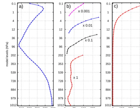
In addition to the σ coordinate, the stability profile de-fined by Eq. (8) is another required input to the program for the computation of the vertical structure functions. For the hybrid coordinate of the ECMWF model and several cli-mate models (e.g. NCAR clicli-mate model, EC-Earth) values of σ are readily obtained from the available values of average full and half-level pressures. In order to compute the stabil-ity profile, globally averaged temperatureT0on eachσlevel needs to be specified. The profile ofT0presented in Fig. 2a is computed from ERA Interim reanalyses for the year of 2000 but it varies little if a multi-year period is used. The same applies for the stability profile computed by Eq. (8) from dT0/dσ and theσ levels. The profile of00for ERA Interim is presented in Fig. 2b. It can be seen that the values of00 are positive and they vary little throughout the troposphere; however, in the upper stratosphere and the mesosphere 00 increases significantly so that overall it can vary several or-ders of magnitude between the surface and 0.1 hPa. As a re-sult, the stability parameter Swhich is computed for use in Eq. (10) has a profile with values rapidly increasing in the upper stratosphere (Fig. 2c).
Appendix B shows parameters in the input namelist
vs-fcalc_cnf needed for the computation of vertical structure
functions. The input file with namelists is vsfcalc.cnf. In ad-dition to the two binary input files, a user specifies the names of two output files which will contain the vertical structure functions and equivalent depths. In principle, the number of vertical modes, which correspond to the number of vertical structure functions saved in the output file, is the same as the number of vertical sigma levels. However, one may not want to use all vertical structure functions in the projection due to small equivalent depths associated with higher verti-cal modes. As seen in Fig. 3 showing vertiverti-cal structure func-tions for ERA Interim, equivalent depths range from about
N. Žagar et al.: Normal-mode function representation: software description and applications 21
210 230 250 270 290 1012
979 884 728 539 353 202 96 36 12 4 1 0.1
model levels (hPa)
T0 (K) a)
0 75 150 225 1012
979 884 728 539 353 202 96 36 12 4 1 0.1
x 1 x 0.1 x 0.01 x 0.001
Γ0 (K) b)
0 150 300 450 1012
979 884 728 539 353 202 96 36 12 4 1 0.1
S c)
Figure 2. Globally-averaged vertical profiles of (a) temperature, (b) stabilityΓ0and (c) normalized stability parameterSon model levels
which is input to the vertical structure equation (10). Profiles are based on ERA Interim model-level data for year 2000. Labels ony-axis are
average pressures of the model levels. Values of stability at various levels in (b) are scaled by different factors for clarity reasons. Under 200 hPa stability is not scaled.
Figure 2. Globally averaged vertical profiles of (a) temperatureT0,
(b) stability00and (c) normalized stability parameterSon model
levels. The stability profile is input to the vertical structure equa-tion (10). Profiles are based on ERA Interim model-level data for year 2000. Labels on y axis are average pressures of the model lev-els. Values of stability at various levels in (b) are scaled by different factors for clarity reasons. Under 200 hPa stability is not scaled.
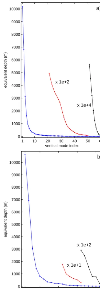
D=10 km down to centimetres or even millimetres. There is a rapid drop in values of equivalent depth after the lead-ing five vertical modes. In the case of ERA Interim presented in Fig. 3, there are four equivalent depths greater than 1 km, 11 equivalent depths between 1 km and 100 m while further 18 equivalent depths have values greater than 10 m. Between 10 and 1 m there are 14 depths and the remaining 13 values of equivalent depth are between 1 m and 4 mm. These values defineMvalues of the constantγ(Eq. 21) forMsystems of the HSEs (18). As illustrated in the next section, the merid-ional extent of the horizontal structure functions is associated with the magnitude ofD. The Hough functions correspond-ing to equivalent depths of the order of 10 m are meridionally bounded to the tropics.
N. Žagar et al.: Normal-mode function representation: software description and applications 1179
22
N. Žagar et al.: Normal-mode function representation: software description and applications
1 10 20 30 40 50 60
0 1000 2000 3000 4000 5000 6000 7000 8000 9000 10000
vertical mode index
equivalent depth (m)
x 1e+2
x 1e+4
a)
1 5 10 15 20
0 1000 2000 3000 4000 5000 6000 7000 8000 9000 10000
vertical mode index
equivalent depth (m)
x 1e+1 x 1e+2
b)
Figure 3. Values of the equivalent depths obtained as solution of the vertical structure equation for ERA Interim modelling system. (a) 60 model levels and (b) 21 model levels closest to the standard 21 pressure levels. A part of equivalent depths in (a) is also shown multiplied by factor 100 (modes 21-50) and by factor 10000 (modes 51 to 60). A part of aquivalent depths in (b) is similarly multiplied by factor 10 (modes 11-16) and by f actor 100 (modes 16 to 21).
Figure 3. Values of the equivalent depths Dobtained as solution of the vertical structure equation for ERA Interim modelling sys-tem: (a) 60 model levels and (b) the 21 model levels closest to the standard 21 pressure levels. A part of equivalent depths in (a) is also shown multiplied by factor 100 (modes 21–50) and by factor 10 000 (modes 51 to 60). A part of equivalent depths in (b) is similarly mul-tiplied by factor 10 (modes 11–16) and by factor 100 (modes 16 to 21).
As discussed in previous papers, the equivalent depth for the first vertical mode (m=1) depends only on the surface temperature, which is a global constant, and the model
ver-tical depth (Cohn and Dee, 1989). The equivalent depths for m >1 are relatively insensitive to the value of the surface boundary condition, but they are sensitive to the stability and the depth of the top model layers (Staniforth et al., 1985). In the case of ERA Interim, there are on average 12 levels beneath 850 hPa, 10 levels from 850 to 500 hPa and 13 lev-els between 500 and 100 hPa. The remaining 25 levlev-els are in the stratosphere (21 levels under 1 hPa) and mesosphere (4 levels above 1 hPa). If instead of 60 hybrid models levels we select only the 21 levels closest to the standard-pressure levels, the corresponding equivalent depths are different for higher vertical modes as can be seen in Fig. 3b.
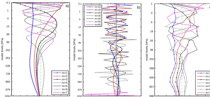
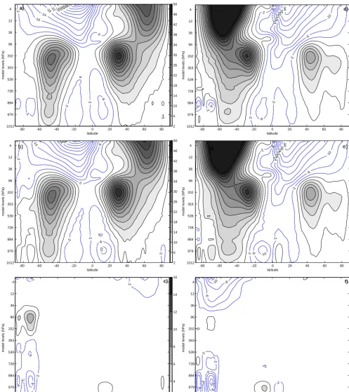
The shapes of vertical structure functions for the ERA In-terim 60-level system are shown in Fig. 4a and b for the first seven vertical modes (Fig. 4a) and for selected higher modes (Fig. 4b). The solutions for first seven vertical modes are also shown for the case of 21 levels (Fig. 4c) defined by values of average pressure closest to the standard pressure. This figure can be compared with other figures from literature includ-ing plots from KP1981 and Žagar et al. (2009a). Each ver-tical modemis associated withm−1 zero crossings in the vertical profile. Therefore, the modem=1, which does not change sign, has traditionally been commonly referred to as the barotropic mode. Lower modes have larger amplitudes in the troposphere and the stratosphere, whereas the relevant structure ofGmfunctions moves downward towards the
sur-face as the value ofmincreases (Fig. 4b). We note that the second mode has its single zero crossing at around 30 hPa and that the leading seven modes have no zero crossings un-der 300 hPa. Traditionally, these modes have been referred to as the first baroclinic mode, the second baroclinic mode, etc., on in the discussion of tropospheric circulation. How-ever, such terms are not suitable in the present case of mod-els with model top levmod-els high above the tropopause. Since several vertical modes correspond to the traditional picture of the first baroclinic mode, using any one of them provides an incomplete picture of the circulation associated with the first baroclinic mode. Instead, we need to sum a number of vertical modes in order to discuss representative circulations in physical space.
3.3 Computation of the horizontal structure functions A separate program computes the meridional structure of Hough harmonics, i.e. vectorsUkn(φ),Vkn(φ)andZkn(φ)for a range of valuesk and n for each equivalent depth. Ap-pendix C shows parameters which need to be specified in the input file houghcalc.cnf via several namelists. Two input
namelists, meridional_grid and vsf_cnf, are previously
1180 N. Žagar et al.: Normal-mode function representation: software description and applications
N. Žagar et al.: Normal-mode function representation: software description and applications 23
-0.4 -0.3 -0.2 -0.1 0 0.1 0.2 0.3 0.4 1012
979 884 728 539 353 202 96 36 12 4 1 0.1
model levels (hPa)
a)
m=1 m=2 m=3 m=4 m=5 m=6 m=7
-0.8 -0.6 -0.4 -0.2 0 0.2 0.4 0.6 1012
979 884 728 539 353 202 96 36 12 4 1 0.1
model levels (hPa)
b) m=10
m=15 m=20 m=30 m=40 m=50 m=60 c)
-0.6 -0.4 -0.2 0 0.2 0.4 0.6 0.8 998
857 500 288 202 96 55 19 6 3 1
model levels (hPa)
c)
m=1 m=2 m=3 m=4 m=5 m=6 m=7 c)
Figure 4. Vertical structure functions for (a) first seven vertical modes and (b) modes 10, 15, 20, 30, 40 50 and 60, derived for 60 model levels of ERA Interim. (c) As (a) but for the case of 21 model levels closest to the standard 21 pressure levels.
Figure 4. Vertical structure functions for (a) the first seven vertical modes and (b) modes 10, 15, 20, 30, 40 50 and 60, derived using the 60
model levels of ERA Interim; (c) same as (a) but for the 21 model levels closest to the standard 21 pressure levels.
maxl). Currently, the same value of meridional modes maxl
applies to all three motion types, EIG, WIG and ROT modes, so that the total number of meridional modes isR=3×maxl.
The namelist output defines the name of the output files with Hough meridional profiles and how the outputs are stored (binary or text format). Further explanations are provided in Appendix C.
The size of output binary files can be relatively large if a large zonal and meridional truncation is requested. For ex-ample, for the presented ERA Interim data set, we have used 200 zonal wave numbers and 70 meridional modes for each of the IG and balanced modes. With a single file per zonal wave number, there are as many files with meridional struc-ture of Hough function as zonal wave numbers. The com-putation of horizontal structure functions is also the most memory intensive computation. However, once these files are computed, they can be used repeatedly for projection pur-poses and they are read only once at the beginning of projec-tion and filtering.
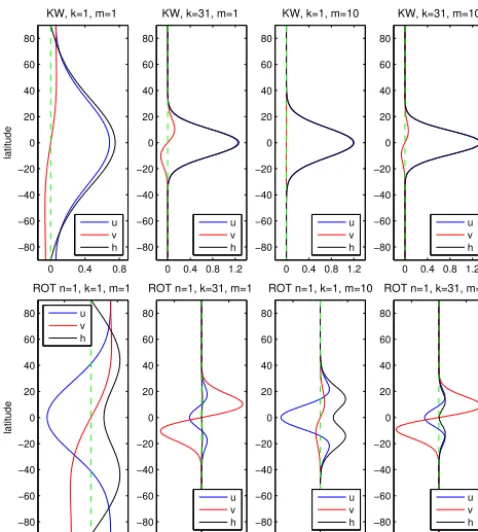
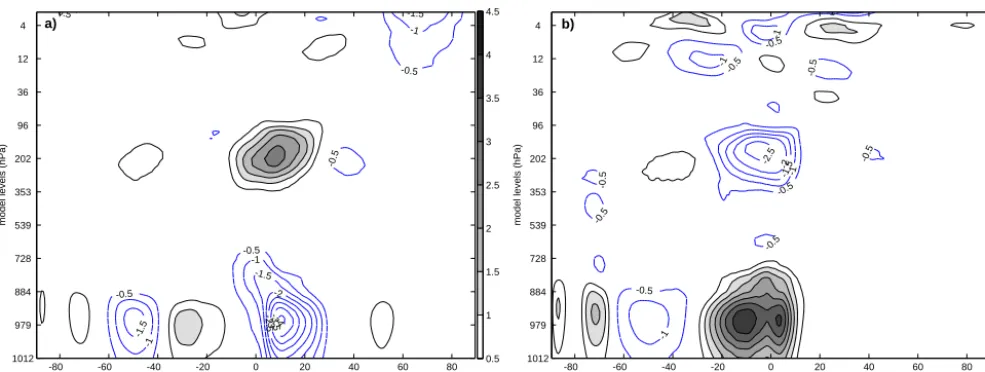
The meridional profiles of the Hough functions corre-sponding to the Kelvin mode and to then=1 balanced mode are shown in Fig. 5 for two zonal wave numbers and for two vertical modes. The displayed vertical modesm=1 and m=10 have equivalent depths of ca. 10 km and 220 m, re-spectively. We can see that an increased value of the vertical mode index, i.e. a reduced value of equivalent depth is as-sociated with a stronger equatorial trapping of the horizontal structure functions. Similar equatorial trapping of horizon-tal structure functions occurs when the zonal wave number increases for the same equivalent depth. In Fig. 5 the solu-tion for (k,m)=(1,10) appears equatorially trapped nearly as much as the solution for (k,m)=(31,1). For the barotropic mode, the horizontal structure of all modes is global. This
tells us that the Hough functions associated with small equiv-alent depths are strongly bounded to the Equator and hence not useful for the projection of data in the extra-tropical re-gions. Furthermore, these numerically obtained small equiv-alent depths are associated with vertical structure functions that are representative only of the lower troposphere and the boundary layer. Therefore, even if one can solve the VSE for all vertical modes, the number of vertical modes we keep in the computation of the horizontal structure functions (param-eter num_vmode in namelist vsf_cnf in Appendix C) should in principle be smaller than the number of model levels. For the results presented in the next section for ERA Interim, we kept 43 vertical modes with equivalent depths greater than 1 m. While it is not wrong to keep all vertical modes, we found that not using vertical modes with equivalent depth smaller then 1 m is a good option in the case of models with many vertical levels such as the ECMWF model.
3.4 Projection of 3-D data on normal-mode functions
Namelists for the meridional grid and vertical structure
func-tions defined in previous subsecfunc-tions are also used in the input file normal.cnf for the projection that is given in Ap-pendix D. In addition, namelist hough_cnf specifies input files with the meridional Hough functions while the remain-ing namelists provide information about the input data. The user can choose to save the globally averaged vertical tem-perature profileT0 and surface pressure field. These can be used for a posteriori interpolation from sigma levels back to the hybrid (or other) model levels or for the computation of temperature perturbations from the geopotential pertur-bations. Namelist input_data describes the data format and the vertical grid. The data valid for a single time step can be contained in several files which together must contain
N. Žagar et al.: Normal-mode function representation: software description and applications 1181
0 0.4 0.8 1.2
−80 −60 −40 −20 0 20 40 60 80
KW, k=31, m=1
u v h
0 0.4 0.8 1.2
−80 −60 −40 −20 0 20 40 60 80
KW, k=1, m=10
u v h
0 0.4 0.8 1.2
−80 −60 −40 −20 0 20 40 60 80
KW, k=31, m=10
u v h
0 0.4 0.8
−80 −60 −40 −20 0 20 40 60 80 latitude
KW, k=1, m=1
u v h
−1 −0.5 0 0.5
−80 −60 −40 −20 0 20 40 60 80 latitude
ROT n=1, k=1, m=1
u v h
−1 0 1
−80 −60 −40 −20 0 20 40 60 80
ROT n=1, k=31, m=1
u v h
−1 0 1
−80 −60 −40 −20 0 20 40 60 80
ROT n=1, k=1, m=10
u v h
−1 0 1
−80 −60 −40 −20 0 20 40 60 80
ROT n=1, k=31, m=10
u v h
Figure 5. Meridional structure of the Hough harmonics for (top)
Kelvin mode and (bottom) n=1 balanced mode. The four
pan-els for each mode correspond to various combinations of the zonal
wave numberkand vertical modem, as defined in each panels’ title.
fields of temperature, wind components and specific humid-ity on model levels as well as surface pressure and orogra-phy. Horizontally, all fields must be on the regular Gaussian grid. Specific humidity is used in the computation of model-level geopotential. An option to use the software without hu-midity data will soon become available in the package. The projection software works in the following way. First, the in-put files with the meridional grid, vertical structure functions and horizontal structure functions are read. This is followed by the reading of the input data. The modified geopotential variable is computed on the input model levels that are sub-sequently interpolated vertically to the predefined sigma lev-els if needed. This provides the input vector X defined by Eq. (31). The vertical projection (34) is carried out first fol-lowed by the horizontal projection (36). The resulting Hough coefficients are saved in the output file with a prefix defined by the variable coef3DNMF_fname which is appended by the date as specified in the namelist time. Currently, the output file is a direct-access binary file but in the near future we plan to make all outputs NetCDF format files. The data read-ing and the projection step are carried out in the loop over time which is defined in the namelist time. The variable dt defines a regular time step between subsequent files. Outputs of the projection of 30 years of ERA Interim data (once per day at 12:00 UTC) are presented in the next section.
3.5 Filtering of modes to physical space
The inverse projection or filtering of modes back to physical space is defined by Eqs. (35) and (32) for the inverse horizon-tal and vertical projections, respectively. Not all modes need to be inverted back to physical space. For example, it may be of interest to separate the balanced and IG components of circulation. Tropical modes are of special interest as many studies deal with the characteristics of the Kelvin mode and MRG mode throughout the tropical atmosphere. The NMF software can filter any mode or a set of modes back to phys-ical space.
Appendix E contains an example of input file
nor-mal_inverse.cnf for the filtering of a selected range of
(k, n, m) modal indices. In addition to several namelists shared with the file normal.cnf, two namelists,
nor-mal_cnf_inverse and filter_cnf are needed specifically for the
filtering purpose. The former is similar to normal_cnf as it defines the input and output file names and formats. The lat-ter defines the range of the zonal, meridional and vertical modes which are to be filtered. The meridional filtering range is defined separately for the EIG, WIG and balanced modes. If the filtering range is specified in terms of the zonal wave numbers or vertical modes, the range of associated merid-ional modes to be filtered out can be specified by the user. Projection of all modes back to physical space is achieved by choosing the index value of the starting mode to filter (e.g.
eig_n_s) greater than the truncation value for the same mode
(i.e. eig_n_s>maxl). In the next section we shall discuss
out-puts of filtering of the balanced and IG circulation.
4 Modal analysis of ERA Interim: climatological properties
We now present some average properties for the ERA In-terim (Dee et al., 2011) 30 year period 1980–2009. Daily in-put data valid at 12:00 UTC were specified on a 512×256 horizontal grid and 60 vertical levels. Projected fields con-tainingχnk(m)coefficients were saved to files using the pa-rameters provided in Appendix D. The presented climato-logical properties are obtained in several ways. The global energy distributions presented in Figs. 6–8 were obtained by averaging energy in a single zonal wave number and merid-ional mode as defined by Eqs. (47) and (48), respectively. Zonal averages, cross-equatorial flow and horizontal circu-lation on selected levels were produced by averaging coeffi-cientsχnk(m)over the 30 year period for each mode followed by the inverse projection to physical space based on filtering criteria. Appendix E provides an example of a namelist for filtering the IG circulation.
4.1 Scale-dependent energy distribution
1182 N. Žagar et al.: Normal-mode function representation: software description and applications
N. Žagar et al.: Normal-mode function representation: software description and applications 25
1 2 3 5 7 10 15 25 50 100 180
10-2
100
102
104
zonal wave number
Energy (J/kg)
a)
-1
-3 -5/3
Total energy Balanced energy (ROT) Inertio-gravity energy (IG)
1 2 3 5 7 10 15 25 50 100 180
10-2
10-1
100
101
102
zonal wave number
Energy (J/kg)
b)
IG
Easterly IG (EIG) Westerly IG (WIG)
1 2 3 5 7 10 15 25 50 100 180
10-4
10-2
100
102
zonal wave number
Energy (J/kg)
c)
-5/3
ROT n=0 ROT n=1 ROT n=3 ROT n=5 ROT n=11
Figure 6. Atmospheric energy spectra. (a) Energy distribution in balanced (red line) and inertio-gravity (blue line) motions and their sum (total wave energy, in black) as a function of the zonal wavenumber. (b) As (a) but IG (black), EIG (red) and WIG (blue). (c) As (a) but balanced spectra for meridional modesn= 0,1,3,5,11. Spectra are obtained by averaging 30 years of outputs from ERA Interim, 12 UTC analysis. Summation is performed over (a,b) all(m, n)and (c) allmand the mean state (k= 0) is not in-cluded. Short dashed lines (black) correspond to the spectra with slopes−3,−1and−5/3as written next to the lines.
Figure 6. Atmospheric energy spectra. (a) Energy distribution in
balanced (red line) and inertio-gravity (blue line) motions and their sum (total wave energy, in black) as a function of the zonal wave number; (b) same as (a) but IG (black), EIG (red) and WIG (blue);
(c) same as (a) but balanced spectra for meridional modesn=0, 1, 3, 5, 11. Spectra are obtained by averaging 30 years of outputs from ERA Interim, 12:00 UTC analysis. Summation is performed
over (a, b) all(m, n)and (c) allmand the mean state (k=0) is not
included. Short dashed lines (black) correspond to the spectra with
slopes−3,−1 and−5/3 as written next to the lines.
26 N. Žagar et al.: Normal-mode function representation: software description and applications
0 30 60 90 120 150 180
0 0.1 0.2 0.3 0.4 0.5 0.6 0.7 0.8 0.9 1
zonal wave number
Energy ratio
IG/Total ROT/Total
Figure 7. Ratio of balanced (red line) and inertio-gravity (blue line) energy and total energy in each zonal wavenumber. Averaging is performed for 30-year period and for all(m, n).
Figure 7. Ratio of balanced (red line) and inertio-gravity (blue line)
energy and total energy in each zonal wave number. Averaging is
performed for the 30-year period and for all(m, n).
N. Žagar et al.: Normal-mode function representation: software description and applications 27
0 10 20 30 40 50 60 70
100 101 102 103
meridional mode
Energy (J/kg)
Total ROT IG
Figure 8. Distribution of total, balanced and inertio-gravity wave energy in meridional modes. Summation is performed over all (m, k)and the mean state (k= 0) is not included.
Figure 8. Distribution of total, balanced and inertio-gravity wave
energy in meridional modes. Summation is performed over all
(m, k). The mean state (k=0) is not included.
are shown up to the maximal truncation used for the projec-tion: zonal wave number 200, which corresponds to a grid spacing about 100 km at the Equator and about 70 km in mid-latitudes. One can see that the total energy spectra follows the −3 law all the way from the synoptic scales (k >5) down to the smallest analyzed scale. As in Žagar et al. (2009a), we note a major difference between the balanced and unbalanced energy spectra; the latter are characterized by a flatter slope, especially on planetary and synoptic scales. Furthermore, IG energy is not equally split into EIG and WIG contributions, as shown in Fig. 6b. On planetary scales, the EIG dominate. This is largely due to a contribution of KWs as noted in the previous study (Žagar et al., 2009b, c).
en-N. Žagar et al.: Normal-mode function representation: software description and applications 1183 ergy injected at scales associated with baroclinic instability
inversely cascades to larger scales (Charney, 1971). The en-ergy scaling law in planetary scales appear closer to−1 than to the theoretically expected −5/3 law (e.g. Lilly, 1973). Further details about this part of the spectrum can be dis-cussed in relation to Fig. 6c which shows the balanced en-ergy spectra for different meridional modes. The MRG spec-trum (denoted n=0 ROT) appears flat at planetary scales, a feature noticed also in operational ECMWF analyses by Žagar et al. (2009b). The balanced energy spectra for merid-ional modes 1–5, which represent the majority of variability in midlatitudes, have a−5/3 slope as expected by the quasi-geostrophic turbulence theory (Charney, 1971; Tung and Or-lando, 2003).
The total energy distribution shows no sign of slope flattening in sub-synoptic scales in comparison to synop-tic scales. On the contrary, after a zonal wave number of around 100 the total energy spectrum becomes somewhat steeper (Fig. 6a). This lack of variability in sub-synoptic scales has been noted also in other studies of NWP mod-els (e.g. Frehlich and Sharman, 2008) including the NMF re-sults of various analysis systems (Žagar et al., 2009a). One can also notice in Fig. 6a that the slope of IG energy spec-tra becomes steeper as the horizontal scale reduces. In sub-synoptic scales, the IG energy clearly dominates over bal-anced energy.
A relative contribution of the two energy components is further presented in Fig. 7. This figure shows that at the zonal wave numbers 28–30, which correspond to the resolution of about 700 km at the Equator and to around 500 km in the midlatitudes, the unbalanced component of energy becomes greater than the balanced component. Given the global 3-D nature of our spectra and a lack of previous similar inves-tigations, it is difficult to discuss the origin of this scale in ERA Interim data and its realism. A similar scale has been known from observations as the scale of the major shift in the slope of energy spectra (derived for both wind and tem-perature data) from a−3 to−5/3 range (Nastrom and Gage, 1985). However, a similar change of the slope of the total en-ergy spectra is absent in Fig. 6. Furthermore, enen-ergy spectra derived from models are usually based on single level data (e.g. Burgess et al., 2013; Blažica et al., 2013) and they show only kinetic energy; correspondingly, their comparison with the spectrum in Fig. 6a which represents the vertically inte-grated total energy is not simple. Blažica et al. (2013) showed that on mesoscale in midlatitudes the divergent component of kinetic energy is at least equally as large as the rotational component and that the slopes of the corresponding spectra depend on the altitude (see also Burgess et al., 2013). In our global case with the tropics dominated by divergent circula-tions, we find that the unbalanced component makes up 80 % or more of the total energy beyond zonal wave number 100 (about 150 km in midlatitudes) (Fig. 7). On planetary scales, the contribution of IG wave energy is about 10 % or less of the total wave energy in these scales. However, as the
large-scale energy contains most of the energy, the overall contri-bution of unbalanced energy to total energy is somewhat less than 10 %. In planetary scales alone (zonal wave numbers 1– 5) there is 80 % of total energy; synoptic scales (zonal wave numbers 6 to 15) contain about 15 % of the global total en-ergy while sub-synoptic scales (k >15) contribute about 5 % of the total global energy in ERA Interim (Fig. 7). Since re-analyses such as ERA Interim provide the most reliable pic-ture of the general circulation, the numbers above can be used to evaluate the energy distribution in climate models.
The meridional energy distribution is presented in Fig. 8. The dominance of balanced energy over IG energy is clearly seen for all meridional modes except for the lowest,n=0. The reason is that the lowest meridional mode for EIG modes is the Kelvin mode while the MRG wave is saved asn=0 balanced mode. The KW is the most energetic unbalanced mode of the global atmosphere (Žagar et al., 2009b) and its energy level, especially when shown together withn=0 WIG mode, exceeds the energy level of the MRG mode. The balanced energy distribution has a peak in meridional modes n=3–7 which have the most significant structure in the mid-latitudes (not shown). Asnincreases, the IG energy compo-nent reduces much more rapidly than the balanced energy component. This can be expected since asn increases, the meridional structure of modes become less and less relevant for the tropics where the IG circulation dominates.
From the physical point of view, it is more complicated to discuss the energy distribution as a function of vertical mode. As discussed in the previous section, it is difficult to discuss a single vertical mode separately except perhaps the barotropic mode. Nevertheless, the vertical energy distribu-tion displays characteristics for the balanced and IG modes that can be physically interpreted. In particular, the verti-cal distribution of IG energy appears related to tropiverti-cal con-vection which generates a majority of tropical IG motions. Several distinct maxima in energy distribution can be as-sociated with free-propagating large-scale IG modes, with deep convection and with convectively coupled waves (fig-ure not shown). An exact physical interpretation of these en-ergy maxima in relation to dominant equatorial waves de-rived from observations can be obtained by filtering these vertical modes back to physical space and comparing their properties with independent observations. This is a subject of a separate paper.
4.2 Average circulation