www.geosci-model-dev.net/7/2477/2014/ doi:10.5194/gmd-7-2477-2014
© Author(s) 2014. CC Attribution 3.0 License.
Development of a semi-parametric PAR (Photosynthetically Active
Radiation) partitioning model for the United States, version 1.0
J. C. Kathilankal1, T. L. O’Halloran2, A. Schmidt3, C. V. Hanson3, and B. E. Law3
1LI-COR Inc. 4647 Superior Street, Lincoln, NE 68504, USA
2Sweet Briar College, Department of Environmental Sciences, Sweet Briar, VA 24595, USA
3Department of Forest Ecosystems and Society College of Forestry, Oregon State University, 321 Richardson Hall, Corvallis,
OR 97331, USA
Correspondence to: J. C. Kathilankal ([email protected])
Received: 22 January 2014 – Published in Geosci. Model Dev. Discuss.: 6 March 2014 Revised: 29 July 2014 – Accepted: 3 September 2014 – Published: 24 October 2014
Abstract. A semi-parametric PAR diffuse radiation model was developed using commonly measured climatic variables from 108 site-years of data from 17 AmeriFlux sites. The model has a logistic form and improves upon previous ef-forts using a larger data set and physically viable climate variables as predictors, including relative humidity, clearness index, surface albedo and solar elevation angle. Model per-formance was evaluated by comparison with a simple cu-bic polynomial model developed for the PAR spectral range. The logistic model outperformed the polynomial model with an improved coefficient of determination and slope relative to measured data (logistic: R2=0.76; slope=0.76; cubic:
R2=0.73; slope=0.72), making this the most robust PAR-partitioning model for the United States currently available.
1 Introduction
Photosynthetically active radiation (PAR) is the 0.4–0.7 µm spectral range that is absorbed by plants and drives the pro-cess of photosynthesis (McCree, 1972). Photosynthetically active radiation at the ground surface has two primary in-coming streams, diffuse and direct, which are significantly affected by the amount of clouds and aerosols in the at-mosphere. These two radiant components differ in the way they transfer energy through plant canopies, thus affecting canopy photosynthesis processes differently than what would occur at the leaf scale (Misson et al., 2005). Increased dif-fuse PAR fraction (the ratio of difdif-fuse or isotropic PAR to to-tal PAR (diffuse+direct beam)) in the atmosphere has been
correlated with higher light-use efficiency and increased CO2
assimilation (e.g., Weiss and Norman, 1985; Gu et al., 1999, 2002, 2003; Knohl and Baldocchi, 2008; Mercardo et al., 2009; Still et al., 2009). Many of these studies utilize models of diffuse radiation (usually in the 0.15 to 4.0 µm shortwave range) to estimate the diffuse fraction rather than direct mea-surements.
Diffuse PAR can be estimated from models that range in complexity from spectral parameterization schemes like SPCTRAL2 (Bird and Riodan, 1986) and SMARTS2 (Gueymard, 1995) to simple linear regression models relat-ing diffuse radiation fraction to extra terrestrial PAR (Hassika and Berbigier, 1998; Tsubo and Walker, 2005). Jacovides et al. (2009) developed a third-order polynomial model after ap-plying a 25-point moving average on clearness index (ktp)
(the ratio of global irradiance to extraterrestrial irradiance) data collected over a three-year period over Athens, Greece. Butt et al. (2010) used a proxy cloud fraction (ratio of cal-culated total solar irradiance at a surface to the measured) to estimate diffuse PAR fraction.
et al., 2001; Oliveria et al., 2002; Jacovides et al., 2006) equations relating clearness index (ktp)to estimate the
dif-fuse fraction (kdp). Reindl et al. (1990) used multiple
regres-sion analysis and identified air temperature, dew point and sine of the solar elevation angle as important parameters de-termining the partitioning of total irradiance into diffuse and direct components. Solar elevation angle and clearness index were used as inputs in models developed by Maxwell (1987) and Skartveit and Olseth (1987). Other parameters used in modeling the diffuse fraction include dew point temperature, albedo and hourly variability index (root mean square differ-ence between the clearness index of an hour in question with respect to its preceding and succeeding hour; e.g., Perez et al. (1992) and Skartveit et al. (1998)). The Boland–Ridley– Lauret (BRL) model (Ridley et al., 2010) uses hourly clear-ness index, apparent solar time, solar elevation angle, daily clearness index and a persistence index similar to the vari-ability index to calculate the diffuse fraction. Muneer and Munawwar (2006) used sunshine fraction, cloud fraction and air mass along with clearness index in predicting the diffuse fraction of global irradiance.
The objective of our study is to develop a simple semi-parametric diffuse PAR model applicable for the US, em-ploying the AmeriFlux (Hargrove et al., 2003) data set of above-canopy observations that have high spatiotemporal resolution. Development of such a model will aid future in-vestigations of the effect of diffuse radiation on photosynthe-sis and light-use efficiency in response to climate. Although diffuse radiation is not regularly measured at all AmeriFlux sites, multiple-year records from 17 sites are available for model development. The model presented here is developed with a data set that is larger and more temporally and spa-tially diverse than any previous efforts, making it the most robust and broadly applicable diffuse PAR model developed to date. The model development is based on the BRL model as the logistic relationship used in this shortwave diffuse ra-diation model can be adopted for the PAR diffuse fraction but with more pertinent drivers. The model is primarily intended for aiding researchers in understanding ecosystem response in terms of carbon and energy exchange in relation to the dif-fuse PAR fraction with data recorded at the site.
2 Methodology and data analysis
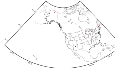
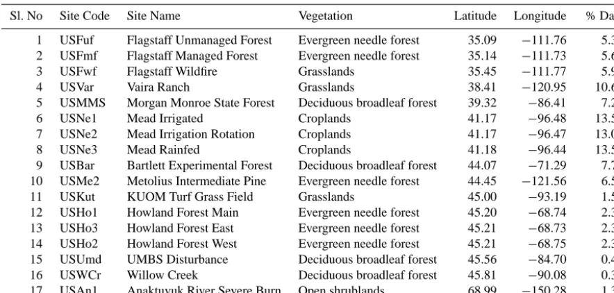
The data set used for model development and testing con-sists of multiple-year records of the PAR and diffuse frac-tion obtained from the AmeriFlux network. A detailed de-scription of the sites utilized in this study is presented in Table 1. The sites selected consist of forested ecosystems, grasslands, shrublands and croplands, covering a wide lati-tude range (35–70◦N). The geographical location of the sites is presented in Fig. 1 in the form of a map. Sites which are close to one another may appear as single points on the map due to the resolution of the map. The diffuse fraction data
Figure 1. Location of sites presented on the USA map. Many sites which are closer together may appear as a single point on the map.
are mostly obtained using the BF3 sensor (Delta-T devices, Cambridge, UK) or a version of it. The BF3 sensor uses an ar-ray of photodiodes with a shading pattern that provides shade to some of the photodiodes while others remain exposed. This instrument has a resolution of 1 µmol m−2s−1 and an accuracy of 15 %. The data from BF3 sunshine recorders have been used in other studies relating cloud fraction to dif-fuse fraction (Butt et al., 2001).
For our study, data collected when solar elevation an-gles were <10◦ were removed to avoid cosine response issues. Although the data set contained records in hourly and half-hourly formats, we averaged data to obtain hourly values for consistency. The hourly radiation values were checked against the quality controls proposed by the Eu-ropean Commission’s Daylight project. This quality con-trol eliminates data points based on the following criteria:
Rd>1.1;RS,RS>1.2RE;Rd>0.8RE;RS<5 W m−2and Rb> RE, where Rd is the total diffuse radiation,RS is the
total incoming solar irradiance,REis the extra terrestrial
ir-radiance andRbis the direct normal irradiance.
Data points were eliminated when hourly rainfall values were greater than 5 mm, relative humidity values were 100 % or when dew point exceeded air temperature as under these conditions, the measurement accuracy might be affected by water droplets formed on the sensor. Outliers were removed visually after the initial quality check so as to remove bad data which could occur due to electronic noise or instrument malfunction that could produce physically impossible values. After implementing the quality control check, the data set consisted of 293 725 hourly records from 108 site-years.
Extraterrestrial PAR (REP)was calculated with solar
ele-vation angle at a location according to
REP=RC
1+0.033 cos(360td/365)sinβ
, (1)
whereRCis the solar constant (2776.4 µmol m−2s−1,
Table 1. Site location and ecosystem-type information.
Sl. No Site Code Site Name Vegetation Latitude Longitude % Data
1 USFuf Flagstaff Unmanaged Forest Evergreen needle forest 35.09 −111.76 5.36 2 USFmf Flagstaff Managed Forest Evergreen needle forest 35.14 −111.73 5.61
3 USFwf Flagstaff Wildfire Grasslands 35.45 −111.77 5.92
4 USVar Vaira Ranch Grasslands 38.41 −120.95 10.62
5 USMMS Morgan Monroe State Forest Deciduous broadleaf forest 39.32 −86.41 7.24
6 USNe1 Mead Irrigated Croplands 41.17 −96.48 13.52
7 USNe2 Mead Irrigation Rotation Croplands 41.17 −96.47 13.04
8 USNe3 Mead Rainfed Croplands 41.18 −96.44 13.51
9 USBar Bartlett Experimental Forest Deciduous broadleaf forest 44.07 −71.29 7.75 10 USMe2 Metolius Intermediate Pine Evergreen needle forest 44.45 −121.56 6.55
11 USKut KUOM Turf Grass Field Grasslands 45.00 −93.19 1.54
12 USHo1 Howland Forest Main Evergreen needle forest 45.20 −68.74 2.38 13 USHo3 Howland Forest East Evergreen needle forest 45.21 −68.73 2.38 14 USHo2 Howland Forest West Evergreen needle forest 45.21 −68.75 2.38 15 USUmd UMBS Disturbance Deciduous broadleaf forest 45.56 −84.70 0.48 16 USWCr Willow Creek Deciduous broadleaf forest 45.81 −90.08 0.36 17 USAn1 Anaktuvuk River Severe Burn Open shrublands 68.99 −150.28 1.36
3 Model development
The model developed here is similar in structure to the multi-predictor logistic model (BRL) developed by Ridley et al. (2010) for global solar irradiance, except we use addi-tional predictors that directly affect the diffuse fraction, and we also use a considerably larger data set. The predictors in the BRL model include daily clearness index (Kt), sine of
the solar elevation angle (sin β), persistence index (ψ )and apparent solar time (AST).
kd= (2)
1
1+exp(−5.38+6.63kt+0.006 AST−0.007 sinβ+1.75Kt+1.31ψ
The logistical form of the model has been identified as more robust than previously published piecewise-linear or other nonlinear forms (Boland et al., 2001, 2008). The goal of our work is to develop a model that is constrained by more commonly measured micrometeorological variables rather than estimated variables like persistence index. The impor-tant factors considered in this study are PAR clearness in-dex (ktp), relative humidity (RH), albedo (α)and sine of
so-lar elevation angle (sin β). Clearness index is widely used in one-predictor models for PAR partitioning (Jacovides et al., 2009) as it is directly related to cloud fraction. Rela-tive humidity is posiRela-tively related with cloud cover (Walcek, 1994) and a greater diffuse fraction is often associated with higher humidity values. The effect of relative humidity on the relationship between ktp and kdp observed in our data
set is presented in Fig. 1a. The data are binned into lin-early spaced bins of relative humidity classes and they indi-cate increased diffuse PAR fractions associated with higher relative humidity classes. Increased surface albedo resulting from changes in canopy reflectance or presence of snow can
alter the diffuse fraction estimates. Skartveit et al. (1998) proposed a correction for clearness index estimation to ac-count for the multiple reflections occurring between the sur-face and instrument dome when albedo is over 0.15. How-ever, in this study we consider albedo as a contributing fac-tor to the diffuse fraction as multiple reflections between the surface and clouds can enhance the diffuse fraction available for photosynthesis (Campbell and Norman, 2008; Knohl and Baldocchi, 2008; Winton, 2005). Albedo of most vegetated surfaces can reach up to 0.25 and can vary widely as a func-tion of leaf area index, disturbance history and snow cover. The effect of surface albedo on the relationship betweenktp
andkdpis presented in Fig. 2b. The diffuse PAR fraction in
general shows an increasing trend with increased albedo, but the trend shows some variations, probably due to the con-founding effects of other factors. Increased albedo can result in the increased diffuse fraction for the same clearness index compared to lower albedo values. The PAR diffuse fraction model developed in this study takes the logistic form
kdp=
1
1+e−z, (3)
wherezis given as
z=a+bktp+cRH+dα+esinβ, (4)
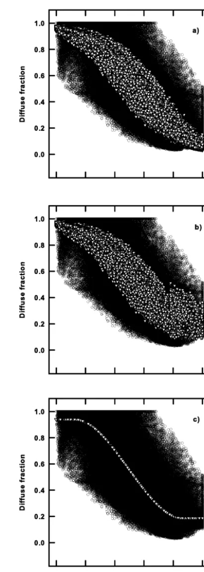
anda,b,c,d ande are fitted empirical coefficients deter-mined in our analysis. The empirical coefficients were ob-tained by fitting the model to the data set. The relationship presented in Eq. (3) tends to underestimate diffuse fraction under clear-sky conditions (Fig. 3a). As a correction, a sec-ond logistic fit is applied to the data for ktp>0.78. The
Figure 2. Relative humidity and albedo effects on thektp−kdp
re-lationship.
Table 2. Logistic model coefficients for clearness index classes. The values given in brackets are the 95 % confidence interval.
Coefficients ktp(≤0.78) ktp(>0.78)
a 2.0196 (2.001, 2.038) 1.2438 (1.161, 1.327)
b −5.6485 (−5.671,−5.626) −2.3335 (−2.400,−2.247)
c 1.3469 (1.331, 1.363) 0.7046 (0.600, 0.729)
d 0.7309 (0.704, 0.758) 0.4107 (0.383, 0.439)
e 0.3045 (0.288, 0.321) −1.9484 (−1.975,−1.923)
model performance is compared with a one-predictor model developed by Jacovides et al. (2009). This model was se-lected for comparison as it was developed using data in the PAR spectral range and used a simple predictor (ktp)that
could be estimated for a large data set from multiple lo-cations. This cubic polynomial model which relates diffuse PAR fraction as a function of smoothed PAR clearness in-dex (moving average window size of 25) takes the following form after fitting to this data set:
kdp = 0.8637+1.2699ktp−5.6676ktp2+3.8088k3tp. (5)
The original cubic polynomial model had prescribed lim-its within which the model operated and constant values were assigned tokdpvalues forktpvalues above and below a
par-ticular range. The modified cubic polynomial model pre-sented in Eq. (5) is valid for 0.13< ktp<0.865, whereas for ktp≤0.125, kdp=0.9399 and ktp≥0.862, kdp=0.18675.
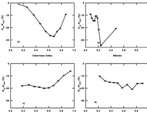
These set points were chosen to provide a smooth transition from the inflection points in the model output. The model co-efficients were estimated using a robust nonlinear regression method in MATLAB (Mathworks, Inc). The fit of data to the adjusted logistic model and the cubic model for the data set is presented in Fig. 3b and c. The percentage differences be-tween the measured diffuse fractionkdpand modeled diffuse
fractionkdpmis plotted in Fig. 4 as a function of each of the
predictor variables in unequally spaced bins with an equal number of data points.
The model fits were assessed by randomly selecting one-third of the data as an evaluation data set for statistical analy-sis. The comparison between measured and modeled diffuse PAR for the logistic and cubical model for the evaluation data
Figure 4. Percentage differences between measured and modeled diffuse radiation as a function of predictor variables.
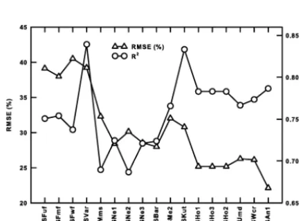
set is provided in Fig. 5. The performance of both models was further compared by using a bootstrap regression be-tween the measured and modeled diffuse fractions with a data re-sampling of 10 000 times to account for the errors in measuring the independent variable (measured diffuse frac-tion) from the evaluation data set. The results of the bootstrap regression comparison for the two models are presented in Table 3. The root mean square error percentage (RMSE %) (Jacovides et al., 2006) of the model fits to the evaluation data set is also presented in Table 3. The influence of seasonality on the logistic model accuracy was examined by plotting the RMSE (%) andR2of the regression between measured and modeled values as a function of the particular months (Fig. 6) for the entire data set. Since seasonality can influence the model fit, the logistic model was fit to the entire data set by classifying the data into the four different seasons. The sea-sons were classified as summer (20 June to 21 September), fall (22 September to 20 December), winter (21 December to 19 March) and spring (20 March to 19 June). This en-abled the development of seasonal model empirical coeffi-cients, which are presented in Table 4. The model fit for the different sites is also presented by plotting the RMSE (%) andR2of the regression between the measured and modeled values for the various sites (Fig. 7). The sites are arranged on thexaxis on an increasing latitudinal gradient and the figure illustrates the model fit across the sites.
4 Discussion
The multi-parameter logistic model predicts different diffuse fractions for the same clearness index for different combina-tions of albedo, solar elevation angle and relative humidity. The percentage difference between the measured and mod-eled diffuse fraction generally indicate an underestimation by
Table 3. Model performance comparison using regression analysis. The values given in the brackets are the standard error of the es-timates obtained by resampling evaluation data 10 000 times. The root mean square error estimate from the measured and modeled values is also presented.
Model statistics Logistic model Cubic model
Slope 0.76 (±6.0×10⁻⁶) 0.73 (±7.0×10⁻⁶) Intercept 0.12 (±4.0×10⁻⁶) 0.13 (±4.0×10⁻⁶) R2 0.76 (±8.0×10⁻⁶) 0.72 (±9.0×10⁻⁶)
RMSE (%) 30.59 32.68
the model. The largest differences are associated with clear-ness index values around 0.67, albedo values of 0.24, mod-erate relative humidity (between 50–60 %) and solar eleva-tion angles of 46◦(Fig. 3). The logistic model thus produces
the largest errors under moderately clear-sky conditions, dur-ing the late morndur-ing and afternoon periods and when the at-mosphere has moderate humidity. The PAR clearness index values close to 0.67 represents a clear-sky condition above which the diffuse PAR fraction stays constant with increas-ing total PAR. The inability of the model to accurately cap-ture this behavior results in large errors around this clearness index threshold. Further higher PAR clearness index values indicate low diffuse PAR fraction levels, which along with the above-mentioned PAR clearness index threshold can lead to uncertainties in the measurement of the diffuse PAR frac-tion by the sensor. The albedo value of 0.24 produced the largest errors as this is in the range of most vegetated surfaces and hence other confounding factors contribute to model er-rors around this albedo range. The cubic polynomial model evaluated in this study produces the largest errors during pe-riods of high solar elevation angle, in contrast to the origi-nal model, which exhibited maximum error during the early morning/late evening hours (Jacovides et al., 2010). The cu-bic polynomial model percentage errors showed a similar be-havior in relation to the clearness index and albedo as the lo-gistic model, but produced the largest errors under low hu-midity in contrast with the logistic model. The regression analysis indicates better performance of the logistic model over the cubic model, with a higher slope, lower intercept and a larger coefficient of determination (R2)(Table 3 and Fig. 5). The RMSE (%) values also indicate a comparatively lower error for the logistic model (30.59 %) compared to the cubic polynomial model (32.68 %). The errors in the devel-oped model could be attributed to other confounding factors such as seasonal effects, changes in atmospheric turbidity caused by air pollution or aerosol loading and location dif-ferences. The fact that a combined data set from different locations was used in this study can lead to minimization of the dependence of the kdp–ktp correlation to local
Figure 5. Comparison between measured and modeled diffuse PAR (a) logistic model (b) cubic polynomial model. The regression statistics presented are for the bootstrap regression between the measure and modeled variables. All units are in µmol m−2s−1.
Figure 6. Logistic model performance in terms of RMSE (%) and
R2over every month of the year.
Figure 7. Logistic model performance in terms of RMSE (%) and
R2over the various sites. The sites are arranged on thexaxis fol-lowing an increasing latitudinal gradient from left to right.
of the seasonal models to the data indicate similarR2 and RMSE (%) values. This indicates the robustness of the lo-gistic model developed in this study as only a marginal im-provement was obtained for certain seasons by determining seasonal coefficients. The largest RMSE (%) values and the lowestR2values were observed for the summer months. The model performance stays constant throughout the year except for the period from September to December when the RMSE (%) values decrease and theR2value increases. The largest RMSE (%) values were observed during the summer months, as in Jacovides et al. (2006) (Fig. 6). The model fit done over the individual sites indicate larger error (higher RMSE (%)) values as latitude increases. The upper latitude experiences lower solar elevation angles which does impact the model accuracy. The lowestR2for the model fit was observed for sites in the middle of the country.
5 Concluding remarks
T able 4. Logistic mo del coef ficients for clearness inde x classes for each season. The v alues g iv en in brack ets are the 95 % confidence interv al. The R 2and the RMSE obtained by comparing the model output to the observ ed data is also pro vided. Model P aram-eter Summer F all W inter Spring ktp ( ≤ 0.78) ktp ( > 0.78) ktp ( ≤ 0.78) ktp ( > 0.78) ktp ( ≤ 0.78) ktp ( > 0.78) ktp ( ≤ 0.78) ktp ( > 0.78) a 2.377 (2.336, 2.418) 1.991 (1.769, 2.214) 2.087 (2.044, 2.130) 1.472 (1.338, 1.606) 1.944 (1.906, 1.981) 0.912 (0.765, 1.060) 2.352 (2.314, 2.389) 2.177 (2.010, 2.343) b − 5.427 ( − 5.467, − 5.387) − 2.834 ( − 3.061, − 2.607) − 5.668 ( − 5.716, − 5.619) − 2.315 ( − 2.450, − 2.180) − 5.463 ( − 5.506, 5.420) − 2.188 ( − 2.339, − 2.038) − 6.143 ( − 6.188, − 6.098) − 3.145 ( − 3.323, − 2.968) c 1.420 (1.390, 1.449) 1.113 (1.060, 1.165) 1.248 (1.211, 1.285) 0.277 (0.232, 0.322) 1.479 (1.443, 1.515) 0.931 (0.886, 0.977) 1.216 (1.186, 1.247) 0.466 (0.420, 0.512) d − 2.200 ( − 2.304, − 2.097) − 2.083 ( − 2.285, − 1.882) 0.347 (0.283, 0.412) 0.656 (0.591, 0.721) 1.141 (1.104, 1.178) 0.497 (0.461, 0.533) − 0.717 ( − 0.808, − 0.627) 0.753 (0.641, 0.866) e 0.032 (0.002, 0.061) − 2.086 ( − 2.141, − 2.032) 0.464 (0.410, 0.518) − 2.535 ( − 2.594, − 2.475) 0.063 (0.022, 0.104) − 1.867 ( − 1.924, − 1.811) 0.796 (0.765, 0.828) − 2.045 ( − 2.086, − 2.005) R 2 0.75 0.77 0.75 0.77 RMSE (%) 31.98 3 0.85 29. 66 29.61 Code availability
The model is a very simple logistic model, and it can be implemented very easily in any programming software or spreadsheet-based software like MS Excel. A MATLAB-based function is provided. This function requires inputs of incoming PAR, relative humidity, albedo and sine of the solar elevation angle.
The Supplement related to this article is available online at doi:10.5194/gmd-7-2477-2014-supplement.
Acknowledgements. This research was supported by the Office of Science (BER), US Department of Energy (DOE, Grant nos. DE-FG02-06ER64307 and DE-FG02-06ER64316). The authors also would like to thank the AmeriFlux Network for providing the data and making it publicly available. We would like to thank the principal investigators of the participating sites and other technical staff who put together this data set and the AmeriFlux QA/QC laboratory at Oregon State University for helping to ensure the quality of data of the AmeriFlux database.
Edited by: R. Sander
References
Bird, R. E. and Riordan, C.: Simple solar spectral model for di-rect and diffuse irradiance on horizontal and tilted planes at the earth’s surface for cloudless atmospheres, J. Climate Appl. Me-teorol., 25, 87–97, 1986.
Boland, J., Scott, L., and Luther, M.: Modelling the diffuse fraction of global solar radiation on a horizontal surface, Environmetrics, 12, 103–116, 2001.
Boland, J., Ridley, B., and Brown, B.: Models of diffuse solar radi-ation, Renewable Energy, 33, 575–584, 2008.
Butt, N., New, M., Malhi, Y., da Costa, A. C. L., Oliveira, P., and Silva-Espejo, J. E.: Diffuse radiation and cloud fraction relation-ships in two contrasting Amazonian rainforest sites, Agr. Forest Meteorol., 150, 361–368, 2010.
Campbell, G. S. and Norman, J. M.: An Introduction to Environ-mental Biophysics, Springer-Verlag, New York, 1998.
Chandrasekaran, J. and Kumar, S.: Hourly diffuse fraction correla-tion at a tropical locacorrela-tion, Solar Energy, 53, 505–510, 1994. De Miguel, A., Bilbao, J., Aguiar, R., Kambezidis, H., and
Ne-gro, E.: Diffuse solar irradiation model evaluation in the North Mediterranean belt area, Solar Energy, 70, 143–153, 2001. Erbs, D. G., Klein, S. A., and Duffie, J. A.: Estimation of the diffuse
radiation fraction for hourly, daily and monthly average global radiation, Sol. Energy, 28, 293–302, 1982.
Gu, L. H., Fuentes, J. D., Shugart, H. H., Staebler, R. M., and Black, T. A.: Responses of net ecosystem exchanges of carbon diox-ide to changes in cloudiness: Results from two North American deciduous forests, J. Geophys. Res.-Atmos., 104, 31421–31434, 1999.
Gu, L. H., Baldocchi, D. D., Wofsy, S. C., Munger, J. W., Michalsky, J. J., Urbanski, S. P., and Boden, T. A.: Response of a deciduous forest to the Mount Pinatubo eruption: Enhanced photosynthesis, Science, 299, 2035–2038, 2003.
Gueymard, C.: Simple Model of the Atmospheric Radiative Trans-fer of Sunshine, version 2 (SMARTS2): Algorithms description and performance assessment, Report FSEC-PF-270-95, Florida Solar Energy Center, 1995.
Hargrove, W., Hoffman, F., and Law, B.: New analysis reveals rep-resentativeness of the AmeriFlux network, EOS, Transactions American Geophysical Union, 84, 529, 2003.
Hassika, P. and Berbigier, P.: Annual cycle of photosynthetically active radiation in maritime pine forest, Agr. Forest Meteorol., 90, 157–171, 1998.
Jacovides, C. P., Tymvios, F. S., Assimakopoulos, V. D., and Kalt-sounides, N. A.: Comparative study of various correlations in es-timating hourly diffuse fraction of global solar radiation, Renew-able Energy, 31, 2492–2504, 2006.
Jacovides, C. P., Boland, J., Asimakopoulos, D. N., and Kalt-sounides, N. A.: Comparing diffuse radiation models with one predictor for partitioning incident PAR radiation into its diffuse component in the eastern Mediterranean basin, Renewable En-ergy, 35, 1820–1827, 2009.
Knohl, A. and Baldocchi, D. D.: Effects of diffuse ra-diation on canopy gas exchange processes in a forest ecosystem, J. Geophys. Res.-Biogeosci., 113, G02023, doi:10.1029/2007JG000663, 2008.
Maxwell, E. L.: A quasi-physical model for converting hourly global horizontal to direct normal insolation, Report SERI/TR-215-3087, Solar Energy Institute, Golden, CO, 1987.
McCree, K. J.: The action spectrum, absorptance and quantum yield of photosynthesis in crop plants, Agr. Forest Meteorol., 9, 191– 216, 1972.
Mercado, L. M., Bellouin, N., Sitch, S., Boucher, O., Huntingford, C., Wild, M., and Cox, P. M.: Impact of changes in diffuse ra-diation on the global land carbon sink, Nature, 458, 1014–1087, doi:10.1038/Nature07949, 2009.
Misson, L., Lunden, M., McKay, M., and Goldstein, A. H.: Atmo-spheric aerosol light scattering and surface wetness influence the diurnal pattern of net ecosystem exchange in a semi-arid pon-derosa pine plantation, Agr. Forest Meteorol., 129, 69–83, 2005.
Muneer, T. and Munawwar, S.: Improved accuracy models for hourly diffuse solar radiation, J. Solar Energy Eng.-Trans. ASME, 128, 104–117, 2006.
Oliveira, A. P., Escobedo, J. F., Machado, A. J., and Soares, J.: Cor-relation models of diffuse solar-radiation applied to the city of Sao Paulo, Brazil, Appl. Energy, 71, 59–73, 2002.
Orgill, J. F. and Hollands, K. G. T.: Correlation equation for hourly diffuse radiation on a horizontal surface, Solar Energy, 19, 357– 359, 1977.
Perez, R., Ineichen, P., Seals, R., and Zelenkal, A.: Dynamic global to direct irradiance conversion models, ASHRAE Transations, 98, 354–369, 1992.
Reindl, D. T., Beckman, W. A., and Duffie, J. A.: Diffuse fraction correlation, Solar Energy, 45, 1–7, 1990.
Ridley, B., Boland, J., and Lauret, P.: Modelling of diffuse solar fraction with multiple predictors, Renewable Energy, 35, 478– 483, 2010.
Skartveit, A. and Olseth, J. A.: A model for the diffuse fraction of hourly global radiation, Solar Energy, 38, 271–274, 1987. Skartveit, A., Olseth, J. A., and Tuft, M. E.: An hourly diffuse
frac-tion model with correcfrac-tion for variability and surface albedo, So-lar Energy, 63, 173–183, 1998.
Spitters, C. J. T., Toussaint, H., and Goudriaan, J.: Seperating the diffuse and direct component of global radiation and its impli-cations for modeling canopy photosynthesis. 1. Component of incoming radiation, Agr. Forest Meteorol., 38, 217–229, 1986. Still, C. J., Riley, W. J., Biraud, S. C., Noone, D. C., Buenning,
N. H., Randerson, J. T., Torn, M. S., Welker, J., White, J. W. C., Vachon, R., Farquhar, G. D., and Berry, J. A.: Influence of clouds and diffuse radiation on ecosystem-atmosphere CO2and
CO18O exchanges, J. Geophys. Res.-Biogeosci., 114, G01018, doi:10.1029/2007JG000675, 2009.
Tsubo, M. and Walker, S.: Relationships between photosyntheti-cally active radiation and clearness index at Bloemfontein, South Africa, Theor. Appl. Climatol., 80, 17–25, 2005.
Walcek, C. J.: Cloud cover and its relationship to relative humid-ity during a springtime midlatitude cyclone, Mon. Weather Rev., 122, 1021–1035, 1994.
Weiss, A. and Norman, J. M.: Partitioning solar radiation into direct and diffuse, visible and near-infrared components, Agr. Forest Meteorol., 34, 205–213, 1985.