Simulation of Position Based Visual Control and
Performance Tests of 6R Robot
M. Habibnejad Korayem i*, A. Habibnejad Korayem, and F. S. Heidari
Received 25 September 2006; received in revised 17 November 2009; accepted 23 February 2010
ABSTRACT
This paper presents simulation and experimental results of position-based visual servoing control process of a 6R robot using 2 fixed cameras. This method has the ability to deal with real time changes in the relative position of the target-object with respect to robot. Also, greater accuracy and independency of servo control structure from the target pose coordinates are the additional advantages of this method. Forward and inverse kinematics of 6R robot have been simulated then simulation of image processing, object recognition and pose estimation of the end effector as well as target-object in Cartesian space and visual control of robot have been prescribed. Performance tests of the 6R robot with two cameras have been simulated. Finally, analysis of error and test data has been carried out according to ISO9283, ANSI-RIA R15.05-2 standards and statistical toolbox of MATLAB. Experimental results obtained from actual implementation of visual control and tests of 6R robot in lab are presented and used to validate simulation tests.
KEYWORDS
Position based visual system, performance, test, robot, simulation
i *
Corresponding Author, Robotic Research Laboratory, Mechanical Engineering Department in Iran University of Science & Technology, Narmak, Tehran, Iran (email:[email protected])
1. INTRODUCTION
Visual control, also called visual servoing, is a very extensive and mature field of research where many important contributions have been presented in the last decade. [1] The majority of vision guidance for industrial robots is based on the 'look and move' concept. In general, this method involves the vision system cameras snapping images of the target-object and the robotic end effector, analyzing and reporting a pose for the robot to achieve. Therefore, 'look and move' involves no real-time correction of robot path. This method is ideal for a wide array of applications that do not require real-time correction since it places much lighter demands on computational horsepower as well as communication bandwidth, thus having become feasible outside the laboratory. The obvious drawback is that if the part moves between the look and move functions, the vision system will have no way of knowing this in reality. This does not happen very often for fixed parts. Yet another drawback is lower accuracy; with the 'look and move' concept, the final accuracy of the calculated part pose is directly related to the accuracy of the 'hand-eye' calibration (offline calibration to relate camera space to robot space). If the calibration were erroneous so would be the calculation of the pose estimation part.
Gilbert describes an automatic rocket-tracking camera
which keeps the target centered in the camera's image plane by means of pan/tilt controls. [2] Weiss proposed the use of adaptive control for the non-linear time varying relationship between robot pose and image features in based servoing. Detailed simulations of image-based visual servoing are described for a variety of manipulator structures of 3-DOF. [3]
Mana Saedan and M. H. Ang worked on relative target-object (rigid body) pose estimation for vision-based control of industrial robots. They developed and implemented a closed form target pose estimation algorithm. [4]
Skaar et al. used a 1-DOF robot to catch a ball. [5] He proposed a two stage algorithm for catching moving targets. Coarse positioning was performed to approach the target in near minimum time and `fine tuning' to match robot acceleration and velocity with the target.
approaches. [8]
Simulation of behavior and environment of robots have been done in many research activites. Korayem et al. designed and simulated vision based control and performance tests for a 3P robot by visual C++ software. [9, 10] They used a camera which was installed on end effector of robot in feature-based-visual servo system to bring it to the target. But the vision-based control in our work is implemented on 6R robot. The two cameras are mounted on the earth, i.e., the cameras observe the robot which we can call the system “out-hand" (the term “stand-alone" is generally used in the literature). The closed form target pose estimation is discussed and used in the position based visual control. The advantage of this approach is that the servo control structure is independent of the target pose coordinates. This method has the ability to deal with real time changes in the relative position of the target-object with respect to robot as well as having greater accuracy. Image feature points in each image are to be matched and 3D information of the coordinates of the target-object and its feature points are computed by this system.
In this paper, the 6R robot which is designed and constructed in IUST Robotic Research Lab, is modeled and simulated. Then forward and inverse kinematics equations of the robot are derived and simulated. After discussing simulation software of 6R robot, we simulated control and performance tests of robot and finally the results of tests according to ISO9283 and ANSI-RIAR15.05-2 standards and MATLAB are analyzed. 2. THE 6R ROBOT AND SIMULATOR ENVIRONMENT
This 6 DOF robot, has 3 DOF at waist, shoulder and hand and also 3 DOF in its wrist that can do roll, pitch and yaw rotations. First, link rotates around vertical axis in horizontal plane; second link rotates in a vertical plane orthogonal to first link’s rotation plane. The third link rotates in a plane parallel to second link’s rotation plane.
The 6R robot and its environment have been simulated in simulator software, by mounting two cameras in fixed distance on earth observing the robot. These two cameras capture images from robot and surrounding. After image processing and recognition of target-object and end effector, positions of them are estimated in image plane coordinate. Then visual system leads the end effector toward target. To have the end effector and target-object positions in global reference coordinate, the mapping of coordinates from image plan to the reference coordinates is needed. But this method needs camera calibration which is non linear and complicated. In this simulating program, we used a neural network instead of mapping. Performance tests of robot are also simulated by using these two fixed cameras.
3. FORWRD KINEMATICS OF THE 6R ROBOT
According to the Denavit-Hartenberg notation for the 6R robot, the D-H parameters are listed in Table 1.
TABLE 1. KINEMATICS PARAMETERS FOR THE 6R.
α a d θ AXIS
2
/
π
−
0 1d
1 θ 1 0 2a
0 2 θ 2 0 3a
0 3 θ 32
/
π
4a
0 4 θ 42
/
π
−
0 0 5 θ 5 0 0 6d
6 θ 6By multiplying the link transform matrices for the robot the total transformation matrix will be: 06
T
which determines position and orientation of end effector with respect to base coordinate. If positions of joints are determined by position sensors, the pose of end effector will be determined according to06T
. For 6R robot this matrix will be as Equation 1:= 1 0 0 0 6 0 z z z z y y y y x x x x P a o n P a o n P a o n T (1) where: 5 1 6 2 2 23 3 234 4 234 5 6
1(dSC aC aC aC) dSC
C
Px=− − − − − oz=S234C5S6−C6C234
1 2 2 23 3 234 4 234 5
6SS aS aS aS d
d
Pz= − − − + 1 5 6 234 6 234
1 5 6
( )
y
n S C C C S S
CS C = − + 5 1 6 2 2 23 3 234 4 234 5 6
1(dSC aC aC aC) dCC
S
Py=− − − − +
234 6 234 6
5CS S C
C
nz =− −
6 5 1 234 6 234 6 5
1(CCC SS ) SSC
C
nx= − −
5 1 234 5
1SC CC
S
ay=− +
234 1 6 5 1 234 1 5
6(CSC CS ) C SS
S
oy=− + −
5 1 234 5
1SC SC
C ax =− −
6 5 1 234 6 234 6 5
1(CSC CS ) SSS
C
ox =− + + az=S234S5
Using the notational shorthand as follows:
ij j i ij j i i i i
i C Sin S Cos C Sin S
Cosθ = , θ = , (θ +θ )= , (θ +θ )=
4. INVERSE KINEMATICS OF ROBOT
Given a desired position and orientation for the end effector of robot, to find values for the joint angles which satisfy Equation 1, we need to solve inverse kinematics of robot. For 6R robot, inverse kinematics equations will be as follows: π θ θ θ = + − − = − 1 1 6 6 1
1 tan and
a d P a d P x x y y (2) − − − ± = − 1 1 2 / 1 2 1 1 6 1 5 ] ) ( 1 [ tan S P C P S a C a d x y x y θ (3) 0 , 0
tan 5 6 6 5
1 1 1
6 > = + <
− −
= − θ θ θ π θ
θ for and for
S n C n C o S
ox y
π θ θ θ
θ > = +
+ −
= −
234 234 5
1 1 1
234 tan , if 0,else
S a C a
a
y x
z
(5)
+ −
± −
= − −
t u q
w q
w 1
2 / 1 2 1
2 tan
/ ] ) / ( 1 [ tan
θ (6)
3 2 234 4 2 2 2
2 2 1
3 tan θ ,θ θ θ θ
θ − = − −
− −
= −
C a t
S a u
(7,8) where:
2 2 3 2 2 2 2 234 5 6 234 4 1
2 2 234
4 234 5 6 1 1
2 ,
,
a a a u t w S S d S a d p u
u t q C a C S d S P C P t
z y x
− + + = +
− + − =
+ = −
+ + =
The above equations are used to simulate robot motion.
5. SIMULATOR SOFTWARE OF 6R ROBOT
For increasing efficiency of designed robot, packages for simulation and control of its movement are developed. Movement control signals are sent to the robot via an interface system, designed by our team.
A. Control and test simulation software of 6R robot To simulate control and test of 6R robot, we have used object oriented software Visual C++6. This programming language is used to accomplish this plan because of its rapidity and easily changed for real situation. In this software, the picture is taken in bitmap format through two fixed cameras which are mounted on the earth in the capture frame module. It is returned in form of array of pixels. Both of the two cameras after switching the view will take picture. After image processing, objects in pictures are saved separately. Features are extracted and target-object and end effector will be recognized among them according to their features and characteristics. Then 3D position coordinates of target-object and end effector are estimated. After each motion of joints new picture is taken from end effector. This procedure is repeated until end effector reaches the target-object.
With images, positions of objects are estimated in image plane coordinate. In this program, in order to transform coordinates from image plane to 3D global coordinate we used a neural network. Neural networks are used as nonlinear estimating functions. To compute processing matrix, a set of points were used to train the neural system. These collections of points are achieved by moving end effector through different points whose coordinates in global reference system are known. Their coordinates in image plane of the two cameras are computed in pixels by vision module in simulator software. The position of the end effector is recognized at any time by two cameras.
The trained neural network is a back propagation perception with 2 layers. In input layer there are 4 node entrances including picture plan coordination pixels from two fixed cameras, to adapt a very fit nonlinear function. We have used 10 neurons in this layer with tan sigmoid functions. In the second layer (output layer), there are 3 neurons with 30 input nodes and 3 output nodes which are 3D coordinates x, y and z of object in the earth-reference system. This network can be used as a general function approximator. It can approximate 3D coordinates of any points in image plane of two cameras arbitrarily well, with given sufficient neurons in the hidden layer and tan-sigmoid functions.
The performance of trained network is 0.089374 in less than 40 iterations (epochs). A regression analysis between the network response and the corresponding targets is performed. Network outputs are plotted versus the targets as open circles (Fig.1). The best linear fit is indicated by a dashed line. The perfect fit (output equal to targets) is indicated by the solid line. In this trained net, it is difficult to distinguish the best linear fit line from the perfect fit line, because the fit is so good. It is a measure of how well the variation in the output is explained by the targets and there is perfect correlation between targets and outputs. Results for x, y and z directions are shown in Fig.1
(a) (b) (c)
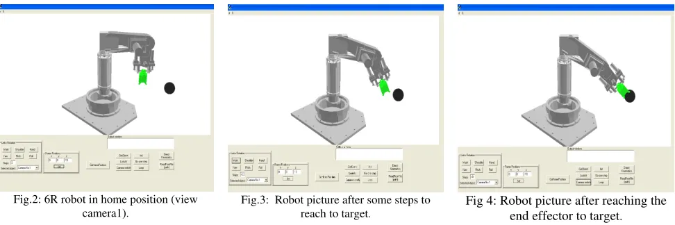
Fig.2: 6R robot in home position (view camera1).
Fig.3: Robot picture after some steps to reach to target.
Fig 4: Robot picture after reaching the end effector to target.
1.Control simulation of 6R robot
To simulate control of 6R robot, the picture is taken in bitmap format by two stationary cameras. Image capturing is switched through two cameras; it means that both cameras take photograph from robot and its surrounding. Images will be processed. After image processing objects in pictures are saved separately and their features are extracted. The target-object and the end effector will be recognized among them according to their features and properties. Then position coordinates of target-object and end effector are estimated. After each motion of joints, new picture is taken from end effector.
Positions of objects are estimated in image plane coordinate. These 2D positions are transformed to global reference coordinate. This approach was used to control the end effector reaching to the target-object and is called position based visual servoing control.
The advantage of this approach is that the servo control structure is independent of the target pose coordinates. Image feature points in each image are to be matched. 3D information of the target-object coordinates and feature points are computed by this system.
In this algorithm, after threshold, segmentation, and labeling, the objects in the pictures will be extracted. After separation of the objects, the target-object and end effector are recognized among them according to their features and properties.
Distance between end effector and target-object will be estimated, by using inverse kinematics equations. Each joint angle will be computed then by revolution of joints end effector will approach to target. In each step cameras take image. This process will repeat until end effector reach to the target; and the distance between target-object and end effector gets the least possible amount. Control procedure of robot to reach to target-object is briefly shown in Figs. 2-4.
2. Robot performance tests simulation
Performance tests of robot including forward and inverse kinematics and motion of end effector in continues paths such as circle, rectangle and line are done.
of end effector is determined in transformation matrix T. Amount of joint angles which satisfy inverse equations will be found. Then wrist will be in desired pose. Two observer cameras take pictures. Pose of end effector will be estimated to determine positioning error of robot.
Using ISO9283, ANSI-RIA standards, these errors will be analyzed and performance characteristics and accuracy of the robot will be determined. In this research, we try to do some of these tests by using camera and visual system according to the standards such as ISO-9283, and ANSI-RIA.
6. PERFORMANCE TEST OF ROBOT ACCORDING TO ISO AND ANSI STANDARDS
The designed robots should accomplish the given tasks accurately and smoothly. This is possible in the case that the motion of the end effector of robot is accurate enough relative to the target-object. The accuracy of actual robot decreases due to different factors. So, in simulator program these errors are figuratively inserted.
Two standards to specify robot performance parameters using camera are ISO and ANSI. We attained parameters of the 6R robot according to both of these standards.
A. Performance tests of 6R robot according to ISO9283 standard
The tests operating to specify robot parameters in this standard are divided into eight categories. In this research, two approaches performed by camera and visual system are implemented to measure the path related parameters of 6R robot.
1. Forward kinematics test of 6R robot (point to point
motion)
In this part of test, pose accuracy and repeatability of robot are determined in directions x, y, z as shown in Fig. 5.
2.Inverse kinematics test
in global reference frame.
By comparing the ideal amount of pose and real one, the positioning error will be determined. Positioning error in directions x, y, z for 10 series of inverse kinematics tests is shown in Fig.7.
1 2
3 4
5 6
7 8
9 10
ex ey
ez -0.5
-0.3 -0.1 0.1 0.3 0.5 0.7 0.9 1.1 1.3 1.5
e
rr
o
r(
m
m
)
Test
ex ey ez
Fig.5: The error schematics in x, y, z directions for forward kinematics tests.
1 2 3 4 5 6 7
8 9 10
ex ez
ey -3
-2 -1 0 1 2
e
rr
o
r
(m
m
)
Test
ex ez ey
Fig. 6: The error schematics in x, y, z directions for inverse kinematics tests.
3.Continuous path test
To determine accuracy of robot in traversing continuous paths, wrist of robot is guided along different paths. In simulator software, 3 standard paths are tested.
a) Direct line
To move end effector along a direct line its start and end points must be determined. Approach vector direction is normal to direction of line path, i.e. , wrist is always normal to its path. Coordinates of end effector in global reference frame is determined. The positioning error is determined by comparing the ideal pose and actual one. Error of robot in traversing direct line path is shown in Fig.7.
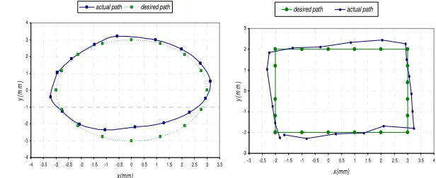
b) Circular path
We investigate the accuracy, repeatability and error of robot on the circular continuous path traversing. Circle is in horizontal plane. Orientation of wrist is so that end effector is always in horizontal plane and normal to circular path. Wrist slides along perimeter of the circle. During motion of wrist on the path, 32 images have been taken. Desired and actual paths traversed by robot are shown in Fig. 8.
c) Rectangular path
Error of motion of the robot’s wrist along rectangular path is also considered. Orientation of end effector is tangent to path. The results are shown in Fig. 9.
-4 -3 -2 -1 0 1 2 3 4 5
-4.5 -4 -3.5 -3 -2.5 -2 -1.5 -1 -0.5 0 0.5 1 1.5
x(mm)
y
(m
m
)
actual path desired path
Fig.7: The error investigated in line paths.
-4 -3 -2 -1 0 1 2 3 4
-4 -3.5 -3 -2.5 -2 -1.5 -1 -0.5 0 0.5 1 1.5 2 2.5 3 3.5
x(mm)
y
(m
m
)
actual path desired path
Fig.8: The error investigated in circular path.
-3 -2 -1 0 1 2 3
-3 -2.5 -2 -1.5 -1 -0.5 0 0.5 1 1.5 2 2.5 3 3.5 4
x(mm)
y
(m
m
)
desired path actual path
Fig.9: The error investigated in rectangular path.
B. Robot performance test based on the American standard ANSI-RIA R15.05-2
The aim of this standard is providing technical information to help users to select the most convenient robot. This standard defines important parameters such as approximate accuracy of the path, absolute accuracy of the path, repetition ability of the path, rapidness specifications, and corner variable. The measurement of these principles brings the opportunity of contrasting
similar robots operations. To make tests more applicable, statistic analysis according to ANSI-RIA standard are performed on the achieved out puts in the former Sections as defined in [11].
7. ERROR ANALYSIS OF THE 6R ROBOT
A. Error analysis according to ISO9283
Pose accuracy (AP) for the robot which means error in positioning and orientation of end effector is computed according to [12]. Position and distance accuracy for 6R robot in different tests are shown in Fig. 10.
Path accuracy of the 6R robot for three paths, line, circle and rectangle is computed in Table 2. In rectangular path tests, cornering round off error (CR) and cornering overshoot (CO) for the 6R robot are also computed. Results are shown in Fig. 11 and listed in Table 2.
B. Error analysis according to standard ANSI-RIA
Maximum and mean path accuracy (AC), Cornering round off error (CR) and Cornering overshoot CO for rectangular path test of 6R robot are calculated. (Table 3)
C. Error analysis with MATLAB
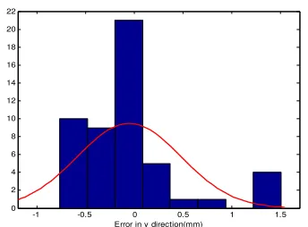
To analyze test errors and compare the results with previous standards we have considered three collections of measured error in x, y and z directions and computed their statistical quantities. For collection of 51 sample errors in x direction, mean value is 0.083 mm, median 0.030 mm, and standard deviation 0.246. Histogram of measured errors in x, y directions are shown in Figs. 12, 13. For collection of 51 measured errors in y direction statistical quantities are computed. Mean value is -0.535 mm, median of errors -0.090 mm, standard deviation is 0.535 mm and maximum of error in y direction is 1.510 mm in positioning of the end effector of robot. Statistical quantities for collection of 51 measured errors in z direction are as follows: Mean value is 0.197 mm, median of errors 0.220 mm, standard deviation is 0.508 mm and maximum of error measured in z direction is 1.320 mm.
A cumulative distribution function is defined as approximation of probability that a measured value has a less amount than or equal to exi. These functions for collections of errors in x, y directions are shown in Figs. 12, 13.
To determine whether or not the measured errors in different directions are symmetrically distributed about the mean we have used skewness ratio. For collection of errors in x direction we have s= skewness (ex) =1.073, in y direction s = 1.340 and for z direction s = -0.107. This negative magnitude means that the distribution is skewed to left and for two previous data, error in x and y directions are skewed significantly to the right.
To show normality of test errors we have superimposed histogram of errors in x, y and z directions with corresponding normal probability distribution function. Results are in Figs. 14, 16. These results can be used to determine whether or not sets of our data can be modeled with normal probability distribution function. If we accept the normal distribution as an adequate representation of errors in x, y and z directions, then we can determine the deviation of our data from normal pdf; results are shown in Figs. 15, 17. It is seen that a fairly large portion of our data are close to the straight line, leading one to conclude that normal distribution is a
1 2 3 4
5 6 7 8
9 10
AP AD
0 0.5 1 1.5 2 2.5
e
rr
o
r(
m
m
)
Test
AP AD
Fig.10: Position and distance accuracy investigated in positioning tests according to ISO9283.
1 2
3 4
5 6
7 8
COi 0.00
0.20 0.40 0.60 0.80 1.00 1.20
e
rr
o
r(
m
m
)
Test
COi CRi
Fig.11: Cornering round off error and cornering overshoot in rectangular path tests according to ISO9283.
TABLE 2. POSE ACCURACY & REPEATABILITY ACCORDING TO ISO9283 STANDARD
AP AD AT CR CO
dir. kin 0.80 0.18 - - -
inv. Kin 0.94 0.43 - - -
line - - 1.12 - -
circle - - 1.33 - -
rectangle - - 1.09 0.47,0.20, 0.17, 0.15
0.72,0.24, 0.17,0.12
TABLE 3. REPEATABILITY & CORNERING OVERSHOOT ACCORDING TO ANSI STANDARD
TEST AC
AC
CR COline 0.67 0.21 - -
rectangle 0.47 0.09 0.47,0.20,
0.17, 0.15
1.03,0.95, 0.17, 0.26
-0.4 -0.2 0 0.2 0.4 0.6 0.8 0
1 2 3 4 5 6 7 8
← Histogram of Error in x dir. Cumulative Distribution→
N
u
m
b
e
r
o
f
O
c
c
u
ra
n
c
e
Measured Error in x direction (mm)
0 0.1 0.2 0.3 0.4 0.5 0.6 0.7 0.8 0.9 1
Mean Value=0.083 Median=0.030 Standard deviation=0.246 No. of samples=51 Min Error=-0.440 Max Error= 0.870
Fig.12: The histogram and cumulative function of error in x direction.
-0.5 0 0.5 1 1.5
0 1 2 3 4 5 6 7 8 9
← Histogram of Error in y dir. Cumulative Distribution→
N
u
m
b
e
r
o
f
O
c
c
u
ra
n
c
e
Measured Error in y direction (mm)
0 0.1 0.2 0.3 0.4 0.5 0.6 0.7 0.8 0.9 1
Mean Value=-0.0533 Median=-0.0900 Standard deviation=0.535 No. of samples=51 Min Error=-0.77 Max Error= 1.510
Fig.13: The histogram and cumulative function of error in y direction.
-0.4 -0.2 0 0.2 0.4 0.6 0.8 0
2 4 6 8 10 12 14 16 18 20 22
Error in x direction (mm)
Fig.14: Histogram with superimposed normal distribution function for error in x direction.
-0.4 -0.2 0 0.2 0.4 0.6 0.8 0.01
0.02 0.05 0.10 0.25 0.50 0.75 0.90 0.95 0.98 0.99
Error Data in x Direction (mm)
P
ro
b
a
b
ili
ty
Normal Probability Plot
error in x dir. best fit area normal pdf
Fig.15: Normal cumulative probability plot of error in x direction.
-1 -0.5 0 0.5 1 1.5 0
2 4 6 8 10 12 14 16 18 20 22
Error in y direction(mm)
Fig.16: Histogram with superimposed normal distribution function for error in y direction.
-0.5 0 0.5 1 1.5
0.01 0.02 0.05 0.10 0.25 0.50 0.75 0.90 0.95 0.98 0.99
Error Data in y Direction (mm)
P
ro
b
a
b
ili
ty
Normal Probability Plot
error in y dir. best fit area normal pdf
Fig.17: Normal cumulative probability plot of error in y direction.
8. EXPERIMENTAL RESULTS AND ANALYSIS
In this part, we represent experimental results for accomplishment of the visual servoing control and performance tests of the 6R robot. To control the robot by vision system, two stationary webcams were installed on the earth watching the robot and environment in front and right view. Brushless DC motors are used in joints of the 6R robot. Maximum velocity of motors is 6000 RPM; after speed reduction in gearbox it is 10 RPM. We have done visual control tests with maximum speed of 10 RPM. Interface processing board analyzes data with speed of 9600 bps. The 6R robot configuration is depicted in Fig. 18.
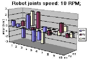
A. Forward kinematics test
In these tests, position accuracy and repeatability of robot is determined. Errors in x, y, z directions for 10 series of forward kinematics tests is depicted in Fig. 19.
B. Continuous path test
Pictures taken by two webcams are saved in bmp format and they are processed through vision algorithm written in VC++. In experimental tests, three standard paths direct line, circle and rectangle are tested Figs. 20- 22.
C. Error analysis based on ISO9283
robot for three paths, line, circle and rectangle is computed in Table 4. In rectangular path tests, cornering round off error (CR) and cornering overshoot (CO) for the 6R robot are also computed.
D. Error analysis based on ANSI-RIA R15.05-2
For rectangular path test of 6R robot the value of CR and CO are calculated. (Table 9-2) The tests were repeated 10 times (n = 10). Corner deviation error (CR) and cornering over shoot (CO) are listed in Table 5.
Fig. 18: 6R robot configuration.
Fig. 19: The error schematics in x, y, z directions for direct kinematics tests of the 6R robot; robot joints speed: 10 RPM.
TABLE 4: POSE, DISTANCE AND PATH ACCURACY ACCORDING TO ISO9283 STANDARD.
TEST AP AD AT CR CO
dir. kin 2.10 1.07 - - -
line - - 1.92 - -
circle - - 2.33 - -
rectangl
e - - 3.01
1.07,4.31, 2.17, 3.24
2.72,4.24, 2.17, 3.02
TABLE 5: POSE ACCURACY & CORNERING OVERSHOOT ACCORDING TO ANSI STANDARD.
TEST AC
AC
CR COline 2.07 1.52 - -
rectangl
e 3.52 3.11
1.47,3.20 , 2.21,
3.15
1.98,3.42 , 2.07,
2.06
circle 1.87 1.47 - -
-40 -35 -30 -25 -20 -15 -10 -5 0
-20 -15 -10 -5 0 5 10 15 20 25 30
X(mm)
Y
(m
m
)
desired path actual path
Fig. 20: The error investigated in experiment of line paths; robot joints speed: 10 RPM.
-40 -30 -20 -10 0 10 20 30 40
-40 -30 -20 -10 0 10 20 30 40
X(mm)
Y
(m
m
)
desired path actual path
Fig.21: The error investigated in circular path; robot joints speed: 10 RPM.
-24 -19 -14 -9 -4 1
14 19 24 29 34 39 44
X(mm)
Y
(m
m
)
desired path actual path
0 0.2 0.4 0.6 0.8 1 1.2 1.4 1.6 1.8 2 2.2
AP AD AT CR CO Experimental Simulation
Fig. 23: Comparison of performance parameters of the 6R robot according to ISO9283 standard in experiments and simulation
results.
0 0.2 0.4 0.6 0.8 1 1.2 1.4 1.6 1.8 2
AC AC CR CO
Experimental Simulation
Fig. 24: Comparison of performance parameters of the 6R robot according to ANSI/RIA standard in experiments and simulation
results.
Performance parameters of the 6R robot in experimental tests and simulated tests are compared in Figs. 23 and 24.
9. CONCLUSIONS
In this paper, it has been shown how to use a position based visual system to control and test the 6R robot. In this system, there is no need to know the first location of robot or object target to calculate the required movement toward the goal. Taken images will help us to estimate the distance of the object to the end effector. This is one of the advantages of this visual system. Also, by applying vision system, the path-related parameters of the robot are found. Robot joints velocity in these tests was 10 rpm. Interface board processed data with 9600 bps speed.
Test errors have been analyzed by using different standards and also MATLAB to compute performance parameters of 6R robot; such as accuracy, repeatability, and cornering overshoot. According to ANSI path accuracy for linear, circular and rectangular paths are: AC= 1.52, 1.47, and 3.11 respectively. According to ISO9283 we had path accuracy PA = 1.92, 2.33, and 3.01. They are fairly close to each other. Also MATLAB showed error data were fairly normally distributed with standard deviation equal to 0.353 and skewness of -0.184.
10. REFERENCES
1. G. Lopez, C. Sagues and J.J. Guerrero, “Homography-Based Visual Control of Nonholonomic Vehicles”, IEEE Int. Conference on Robotics and Automation, Italy, April 2007. pp. 1703- 1708 2. A. Gilbert , M. Giles, G. Flachs , R. Rogers, and H. Yee . “A Real
Time Video Tracking Systems.” IEEE , Trans. Pattern Anal. Mech. Intel. 2(1), pp. 47 – 56 Jan. 1983
3. A. C. Sanderson, L. E. Weiss, and C. P. Neuman. Dynamic visual servo control of robots: an adaptive image-based approach. Proc. IEEE, pages 662.667, 1985.
4. M Saedan and M H Ang Jr, “3D Vision-Based Control of an Industrial Robot”, Proceedings of the IASTED International Conference on Robotics and Applications, Nov 19-22, 2001, Florida, USA, pp. 152-157.
5. S. Skaar,W. Brockman, and R. Hanson. Camera-space manipulation. Int. J. Robot. Res., 6(4):20.32, 1987.
6. J. T. Feddema, C. S. G. Lee, and O. R. Mitchell. Weighted selection of image features for resolved rate visual feedback control. IEEE Trans. Robot. Autom. 7(1):31.47, February 1991. 7. F. Chaumette, P. Rives, and B. Espiau. Positioning of a robot with
respect to an object, tracking it and estimating its velocity by visual servoing. In Proc. IEEE Int. Conf. Robotics and Automation, pages 2248.2253, 1991.
8. H. Hashimoto, T. Kimoto, T. Ebin, “Manipulator Control with Image Based Visual Servoing” In Proc. IEEE, Conf. Robotics and Automation, pp. 2267 – 2272, 1991.
9. M. H. Korayem, N. Shiehbeiki, and T. Khanali, “Design, Manufacturing and Experimental Tests of Prismatic Robot for Assembly Line”, International J. of AMT, Vol. 29, No.3-4, pp. 379-388, 2006.
10. M. H. Korayem, K. Khoshhal, A. Aliakbarpour, “Vision Based Robot Simulation and Experiment for Performance Tests of Robot“, International J. of AMT, Vol. 25, No. 11-12, pp. 1218-1231, 2005.
11. American National Standard for Industrial Robots and Robot Systems Path-Related and Dynamic Performance Characteristics Evaluation. ANSI/RIA R15.05-2. 2002.
12. ISO9283, “Manipulating Industrial Robots Performance Criteria & Related Test Methods”, 1998.