A wavelet method for stochastic Volterra integral equations and its application to general stock model

(1)

A wavelet method for stochastic Volterra integral equations and its

application to general stock model

Saeed Vahdati

Department of Mathematics,

Khansar Faculty of Mathematics and Computer Science, Khansar, Iran.

Abstract In this article, we present a wavelet method for solving stochastic Volterra integral equations based on Haar wavelets. First, we approximate all functions involved in the problem by Haar Wavelets then, by substituting the obtained approximations in the problem, using the Itˆo integral formula and collocating at points then, the main problem converts to a system of linear or nonlinear equation which can be solved by some numerical methods like Newton’s or Broyden’s methods. The capability of the simulation of Brownian motion with Schauder functions which are the integration of Haar functions enables us to find some reasonable approximate solutions. Two test examples and the application of the presented method for the general stock model are considered to demonstrate the efficiency, high accuracy and the simplicity of the presented method.

Keywords. Haar Function, Schauder Function, Haar Wavelet, Itˆo Integral, Brownian Motion. 2010 Mathematics Subject Classification. 65T60, 60H20, 60H35, 60J65.

1. _Introduction

Linear, nonlinear Volterra integral equations and integro-differential equations have an important role in theoretical physics and other disciplines. Several numerical ap-proaches have been suggested for solving these equations, one can find an overview in the monograph. Beginning from 1991 onwards, some numerical methods based on wavelet theory has been applied for solving integral equations. A short investigation

on these papers can be found in [12]. The solutions by these methods are often quite

intricate and the merits of the wavelet method get lost, therefore, some researchers tried to find a simplified version of these methods. One way to do this, is to make use of the Haar wavelets, the most simple wavelets. An overview of the using of Haar wavelet method for solving linear integral equations related to a different and

nonlin-ear Fredholm integral equations can be found in [12] and [13] respectively. Operational

matrix of integration based on Haar wavelets and its application to analyse lumped

and distributed-parameters dynamic systems established and formulated in [6]. For

some other kind of wavelets such as Legendre multi-wavelets and their application

one can refer to [1,2, 8,12,13].

Received: 11 August 2016 ; Accepted: 14 December 2016.

(2)

Many problems in finance, mechanics, biology, medical, social sciences etc can be modeled by stochastic integral equations. The application of the stochastic integral equations for the modeling of such problems makes the study of these problems very useful and there is an increasing demand for studying the behavior of a number of sophisticated dynamical systems in physical, medical and social sciences, as well as in engineering and finance. The mentioned systems are usually dependent on a noise source, such as Gaussian white noise. For this reason, the modeling of such systems mostly requires the use of various stochastic functional equations. For stochastic

differential equation case one can refer to [9,10,11,14,15,16]. Some applications of

stochastic Volterra and Volterra-Fredholm integral equations and stochastic

integro-differential equations can be found in [7,24,25]. Finding an approximate solution for

such problems by using a numerical method is so important because many cases of

these problems cannot be solved analytically [7,9,10,11,14,15,16,24, 25].

Haar wavelet operational matrix method is utilized for fractional order nonlinear

oscillation equations by Saeed et. al [18]. They obtained the solutions of fractional

order force-free and forced Duffing-Van der Pol oscillator and higher order fractional Duffing equation on large intervals. The combination of signal denoising technology and Hankel transforms algorithm which were both based on Haar wavelet

decom-position is proposed in [23]. Zedan et. al [22] proposed a numerical solution based

on Haar wavelet method for Fredholm integral equations and the system of Volterra integral equations.

Wavelet constitutes a family of functions constructed from dilation and translation

of a single function called the mother wavelet. When the dilation parameteraand the

translation parameterbvary continuously, we have the following family of continuous

wavelets as [5],

Ψa,b(t) =|a|

−1

Ψ

_t₋_b a

, a, b∈_R, a6= 0,

where Ψ is the mother wavelet.

Letα >1, β >0 andl, andkare positive integers and restrict the parametersa

andbto the discrete values asa=α−k, b=lβα−k, so the following discrete wavelets

are obtained

Ψl,k(t) =|a|

k

2 _Ψ _αk_t₋_lβ_,

which form a wavelet basis forL2₍

R). For the case, α= 2 and β = 1 then Ψl,k(t)

forms an orthonormal basis [5].

2. _{Haar wavelet and function approximation}

The Haar wavelet family is

ψn(s) =

     

    

1, ₂kj ≤s <

2k+1 2j+1, −1, 2k+1

2j+1 ≤s < k+1

2j ,

0, elsewhere,

(3)

Table 1. The calculation of indicesn, j, mand kforJ= 2.

J = 3, 2M = 2J+1= 8

n= 1· · ·2M 1 2 3 4 5 6 7 8

j=blog2(n−1)c - 0 1 1 2 2 2 2 m= 2j _- ₁ ₂ ₂ ₄ ₄ ₄ ₄ k=n−m−1 - 0 0 1 0 1 2 3

the integerm= 2j,j= 0,1, ..., J indicates the level of the wavelet;k= 0,1, ..., m−1

is the translation parameter, the integerJ determines the maximal level of resolution

and the index nis calculated by the formula n=m+k+ 1. The minimal value is

n= 2 (then m= 1, k= 0)and the maximal value is n= 2M where M = 2J. The

indexn= 1 corresponds to the scaling function

ψ1(s) =

1, 0≤s <1,

0, elsewhere. (2.2)

It easy to see from what we have defined the indices through this section that for a

fixed positive integern≥2, we have j=blog2(n−1)c,m= 2j andk=n−m−1.

As an example, whenJ = 3 remaining indices are listed in Table 1.

The function ψ2(s) is called the mother wavelet, and all the other Haar Wavelets

family except the scaling function are obtained from the mother wavelets by the operations of dilation and translation. This family of function are orthogonal to each

other, so any functionf(s) which is square integrable in (0,1) can be expressed as an

infinite sum of Haar Wavelets as follow

f(s) = ∞

X

n=1

fnψn(s). (2.3)

It is not difficult to see that the series (2.3) terminates at finite term iff(s) is piecewise

constant and the jumps are at points with a finite binary representation. In other cases, the truncation of the above series is given as an approximation of the function

f(s) for piecewise constant during each subinterval. The orthogonal property of Haar

Wavelet family leads us to find the values offn, n= 1,2,· · · as

f1 =

Z 1 0

f(s)ψ1(s)ds,

fn = 2j

Z 1 0

f(s)ψn(s)ds, n= 2· · ·2M, j=blog₂(n−1)c. (2.4)

Imran Aziz [3] introduced a new algorithm to approximate the Haar wavelet

coeffi-cients. To do this, consider the following collocation points

sp= p−0.5

(4)

Let f(s) be a square integrable function which has been approximated by Haar wavelets as follow

f(s)'f2Mˆ (s) =

2M X

i=1

ˆ

fi,2Mψi(s), (2.6)

substituting the collocation points (2.5) into (2.6) and supposing f = ˆf2M at the

collocation points, we get the following linear system of equations

f(sp) = ˆf2M(sp) =

2M X

i=1

ˆ

fi,2Mψi(sp), (p= 1,2,· · ·,2M), (2.7)

which is a 2M ×2M linear system of equations. The following theorem is used to

find the solution of this system for the unknown coefficients ˆfi,2M. We will show that

ˆ

fi,2M, i= 1,· · ·,2M are the midpoint quadrature weights.

Theorem 2.1. The solution of system (2.7) is given as follows

ˆ

f1,2M = 1

2M

2M X

j=1

f(sj), (2.8)

ˆ

fi,2M = 1

ρi 

 βi

X

p=αi

f(sp)− γi

X

p=βi+1

f(sp)



, (2.9)

i = 2,3,· · · ,2M, where

αi = ρi(σi−1) + 1,

βi = ρi(σi−1) + ρi

2,

γi = ρiσi,

ρi = 2M

τi ,

σi = i−τi, τi = 2blog2(i−1)c.

Proof. See [3] and [21].

Now, consider a square integrable functionf(s, t) of two variabless andt. Using

the Haar wavelet basis, this function can be approximated as follows

ˆ

f2M(s, t) = 2M X

i=1

ˆ

fi,2M(t)ψi(s), (2.10)

with a similar argument to the equation (2.6) and the collocation points given in (2.5),

we have the following system of 2M×2M linear equations

f(sp, t) = 2M X

i=1

ˆ

(5)

The following corollary renders an algorithm for finding the unknown coefficients ˆ

fi,2M(t).

Corollary 2.2. The solution of the system (2.11) is given as follows

ˆ

f1,2M(t) =

1

2M

2M X

j=1

f(sj, t), (2.12)

ˆ

fi,2M(t) = 1

ρi   βi X p=αi

f(sp, t)− γi

X

p=βi+1

f(sp, t)



,

i = 2,3,· · ·,2M, (2.13)

whereτi, σi, ρi, γi, βi andαi are defined in theorem (2.1).

Proof. See [20].

Lemma 2.3. Let f ∈ C2_[0_,_1]_, _kf00_k

∞ ≤ M, {fn,2Mˆ }M be the sequence defined in

(2.8) and (2.9) andfnbe the Haar wavelet coefficient defined in (2.4) then lim M→∞

ˆ

fn,2M =

fn, in particular

ˆ

f1,2M −f1 ≤

M

96M2 and

ˆ

fn,2M −fn ≤

M

192M2, n≥2. Proof. For the case n= 1 we have

ˆ

f1,2M−f1 = 1 2M 2M X j=1

f(sj)− Z 1

0

f(t)ψ1(t)dt = Z 1 0

f(t)dt− 1

2M

2M X

j=1 f(sj)

≤ M

96M2, (2.14)

the last inequality holds due to the error-bound composite midpoint rule of the nu-merical integration.

Now, letn≥2 be a positive integer number. Simply put, in the rest of the article

we putn = ₂kj, ζn =

2k+1

2j+1 and ηn = k+1

2j , where j and k are the integer number

regardingnas shown in Table1.

ˆ

fn,2M −fn = 1 ρn βn P p=αn

f(sp)− γn

P

p=βn+1

f(sp) !

−2jR1

0 f(t)ψn(t)dt ≤ 1 ρn βn P p=αn

f(sp)−2jRζn

n f(t)dt

+ 1 ρn γn P

p=βn+1

f(sp)−2jRηn

ζn f(t)dt

(6)

with some elementary calculations, we have                   

αn= 2M k₂j + 1,

βn= 2M k₂j +

M 2j,

γn= 2M k₂j +

2M 2j ,

ρn= 2M₂j ,

(2.16) and                                   

βn−αn+ 1 = M₂j,

γn−(βn+ 1) + 1 = M₂j,

sp=n+4M1 , p=αn,

sp=ζn− 1

4M, p=βn, sp=ζn+_4M1 , p=βn+ 1,

sp=ηn− 1

4M, p=γn,

(2.17)

by using the equations (2.16), (2.17) and the composite midpoint rule, we obtain

1 ρn βn X

p=αn

f(sp)−2j

Z ζn

n f(t)dt

≤ 2j(ζn−n)

3

24 M₂j

2

= M

192M2, (2.18)

and similarly 1 ρn γn X

p=βn+1

f(sp)−2j

Z ηn

ζn f(t)dt

≤ 2j(ηn−ζn)

3

24 M 2j

2

= M

192M2. (2.19)

By considering equations (2.14), (2.18) and (2.19), we get

lim

M→∞ ˆ

fn,2M =fn.

Theorem 2.4. Let f ∈C2_[0_,_1]_,_kf00_k

(7)

Proof. Haar wavelet family is dense inL2[0,1) which means lim M→∞ f− 2M X n=1 fnψn ₂

= 0, (2.20)

further f− ˆ f2M ₂ ≤ f − 2M X n=1 fnψn+

2M X

n=1

fnψn−f2Mˆ ₂ ≤ f − 2M X n=1 fnψn ₂ + 2M X n=1 fnψn− 2M X n=1 ˆ fn,2Mψn ₂ ≤ f − 2M X n=1 fnψn ₂ + 2M X n=1

fn−fn,2Mˆ ψn ₂ ≤ f − 2M X n=1 fnψn ₂ + M

48M, (2.21)

by using equations (2.20) and (2.21), we can get the desire result.

In the next theorem, we will extend the above idea for a bivariate function. Let

f(s, t) be a square integrable function, by using the Haar wavelet basis, we have

f(s, t) = ∞ X n=1 ∞ X k=1

ψn(s)fn,kψk(t),

where

fn,k = 2jn+jk Z 1

0 Z 1

0

f(s, t)ψn(s)ψk(t)dsdt, (2.22)

jn = blog2(n−1)c, jk = blog2(k−1)c.

On the other hand, we can approximate this function in another way by equation

(2.10)

f(s, t)' 2M X

k=1

ˆ

fn,2M(t)ψn(s),

where ˆfn,2M(t), n = 1,2,· · ·,2M are defined in equations (2.12) and (2.13). Each

function ˆfn,2M(t) also can be approximated as follows

ˆ

fn,2M(t)' 2M X

k=1

ˆ

(8)

where the coefficients ˆfn,k,2M are calculated by equations (2.8) and (2.9), so

f(s, t)' 2M X

k=1 2M X

k=1

ψn(s) ˆfn,k,2Mψk(t),

under some assumptions and the following collocation points, we will show

lim

M→∞ ˆ

fn,k,2M =fn,k,

tq =q−0.5

2M , q= 1,2,· · ·,2M. (2.23)

Lemma 2.5. Let Ω = [0,1]2_, _f _∈_C2_(Ω)_{, I}₍_f_{) :=}R1 0

R1

0 f(s, t)dsdt and Q2M(f) := 1

4M2 2M P

n=1 2M P

k=1

f(sk, tn)wheresk andtk are defined in (2.5) and (2.23), then

|I(f)−Q2M(f)| ≤ 1

96M2

max

(s,t)∈Ω

∂2f ∂s2

+ max

(s,t)∈Ω

∂2f ∂t2 |

.

Proof. In a general case, let Ω = [a, b]×[c, d] and f(s, t) : Ω −→ _R be a square

integrable function. Suppose wj and sj, j = 1,2,· · ·, mare the weights and nodes

regarding one dimension numerical integral insdirection andw0_iandti, i= 1,2,· · · , n

are weights and nodes regarding one dimension numerical integral int direction. Let

F(s) =Rd

c f(s, t)dt, we have

I(f) :=

Z b

a Z d

c

f(s, t)dtds=

Z b

a

F(s)ds

=

m X

j=1

F(sj)wj+Es(F(s))

=

m X

j=1 " n

X

i=1

f(sj, ti)wi0+Et(f(sj, t)) #

+Es(F(s))

=

m X

j=1 n X

i=1

f(sj, ti)wi0wj+ m X

j=1

wjEt(f(sj, t)) +Es(F(s))

= Qm,n(f) +Em,n(f),

where,EsandEtare the errors of one dimension numerical integrations in direction

sandtrespectively and also

Qm,n(f) :=

m X

j=1 n X

i=1

f(sj, ti)w0_iwj,

Em,n(f) := m X

j=1

(9)

are the double numerical integration formula and the error terms. Suppose that the one dimension numerical integration, we have

|Et(f(., t))| ≤E¯t, |Es(F(s))| ≤E¯s,

so

|I(f)−Qm,n(f)| ≤WEt¯ + ¯Es, (2.24)

whereW =

m P

j=1 |wj|.

Now, in our special case, we use the midpoint rule (Q2M(f) =Qn,m(f)) where a=

c= 0, b=d= 1, m=n= 2M, wj =w_i0 = _2M1 , hs=ht= _2M1 wherehs andhtare

the distance between two subsequent points in directionsand t respectively. Using

the assumptionf ∈C2

Ω, it is clear that

¯

Es=

1

96M2_(s,t)max_∈_Ω

∂2_f ∂s2 ,

¯

Et= 1

96M2_(s,t)max_∈_Ω

∂2f ∂t2 .

andW =

m P

j=1

|wj|= 1. Substituting the obtained results in (2.24) will complete the

proof.

Theorem 2.6. Under the above assumptions, including the assumption thatf(s, t)∈ C2

Ω, where Ω = [0,1]2. Suppose max (s,t)∈Ω

|∂2f

∂s2| ≤ M1, max (s,t)∈Ω

|∂2f

∂t2| ≤ M2, then for each

k, n= 1,2,· · ·,2M we have lim

M→∞ ˆ

fn,k,2M =fn,k, in particular

|fn,k,2Mˆ −fn,k| ≤ 1

96M2(M1+M2).

Proof. It is clear to see

ˆ

f1,1,2M = 1

2M

2M X

j=1

ˆ

f1,2M(tj) = 1

4M2

2M X

j=1 2M X

i=1

f(si, tj) =Q2M(f)

= Q2M(f ψ1) =Q2M(f ψ1ψ1), (2.25)

ˆ

f1,k,2M k=2,3,···,2M

= 1

ρk 

 βk

X

p=αk

ˆ

f1,2M(tp)− γk

X

p=βk+1

ˆ

f1,2M(tp)





= 1

2M ρk

2M X

n=1 

 βk

X

p=αk

f(sn, tp)− γk

X

p=βk+1

f(sn, tp) 



(10)

Similarly, we have

ˆ

fn,1,2M n=2,3,···,2M

= 2jn_Q

2M(f ψn) = 2jnQ2M(f ψ1ψn), (2.27)

and

ˆ

fn,k,2M n,k=2,3,···,2M

= 2jn+jk_Q

2M(f ψnψk). (2.28)

By using equation (2.22), equations (2.25)-(2.28) and the lemma (2.5), we have

lim

M→∞ ˆ

fn,k,2M =fn,k, n, k= 1,2,· · ·,2M,

and

|fˆn,k,2M −fn,k| ≤

1

96M2(M1+M2).

Corollary 2.7. With the same argument discussed in (2.4), letΩ = [0,1]2, f(s, t)∈C_Ω2, max

(s,t)∈Ω| ∂2_f

∂s2| ≤ M1, max (s,t)∈Ω|

∂2_k

∂t2| ≤ M2 and

ˆ

f2M(s, t) =

2M P

k=1 2M P

k=1

ψn(s) ˆfn,k,2Mψk(t)then lim

M→∞

f−

ˆ

f2M ₂= 0.

3. _{Simulation of Brownian motion via series representations}

Definition 3.1. Let (Ω,F,_P) be a probability space and let {Ft} be a filtration,

B(t) =Bt=Bt(ω) is a one-dimensional Brownian motion with respect to{Ft}and

the probability measure_P, started at 0, if [4]

(1) BtisFtmeasurable for eacht≥0.

(2) B0= 0, a.s.

(3) Bt−Bsis a normal random variable with mean 0 and variancet−swhenever

s < t.

(4) Bt−Bsis independent ofFswhenevers < t.

(5) Bthas continuous paths.

Since the Brownian sample paths are continuous functions, they can be expanded

in a Fourier series. However, the paths are random functions: for differentωdifferent

functions are obtained. This means that the coefficients of this Fourier series are random variables, and since the process is Gaussian, they must be Gaussian as well.

The representation of Brownian motion on the interval [0,2π] is called Paley-Wiener

representation, which is formulated as follows [17]

Bt(ω) = Z0(ω)√t

2π+

2

√ π

∞

X

n=1

Zn(ω)sin(

nt 2) n , t ∈ [0,2π],

where (Zn, n≥0) is a sequence of iid (independent and identically distributed)N(0,1)

(11)

Another such well-known representation is due to L´evy representation, since the sine functions are replaced by certain polygonal functions (the Schauder function).

Let’s define the Haar functionsHn on [0,1] as follows

H1(t) = 1,

H2m+1(t) =     

   

2m2, if t∈1− 2

2m+1,1− 1 2m+1

,

−2m2, if t∈1− 1 2m+1,1

,

0, elsewhere,

H2m+k(t) =     

   

2m2, if t∈k−1

2m ,

2k−1 2m+1

,

−2m2, if t∈2k−1 2m+1,

k 2m

,

0, elsewhere,

k= 1, . . . ,2m−1; m= 0,1, . . . .

From these functions, define the system of the Schauder functions on [0,1] by

inte-grating the Haar functions

e Hn(t) =

Z t

0

Hn(s)ds, n= 1,2, . . . .

Figure3 shows the graphs of Hn andHne for the first n. A series representation for

Figure 1. The graphs ofHn andHne for the first n.

0 0.2 0.4 0.6 0.8 1

Haar Functions

0 0.2 0.4 0.6 0.8 1

0 0.2 0.4 0.6 0.8 1 -1

-0.5 0 0.5 1

0 0.2 0.4 0.6 0.8 1 -1.5

-1 -0.5 0 0.5 1 1.5

0 0.2 0.4 0.6 0.8 1 -1.5

-1 -0.5 0 0.5 1 1.5

0 0.2 0.4 0.6 0.8 1

Schauder Functions

0 0.2 0.4 0.6 0.8 1

0 0.2 0.4 0.6 0.8 1 0

0.1 0.2 0.3 0.4 0.5

0 0.2 0.4 0.6 0.8 1 0

0.1 0.2 0.3 0.4

0 0.2 0.4 0.6 0.8 1 0

(12)

Brownian sample path on [0,1] is then given by

Bt(ω) = ∞

X

n=1

Zn(ω)Hne (t)t∈[0,1], (3.1)

where the convergence of this series is uniform fort∈[0,1] andZn(ω)s are realizations

of an iidN(0,1) sequence (Zn).Haar wavelet approximation of the involved functions

in the problem, simulation of the Brownian motion by Haar functions and the simi-larities between the Haar wavelet family and Haar functions enable us to reduce the computational costs in solution procedure.

4. _{Stochastic integration operational matrix}

In this section, we have applied the Itˆo integral for functionsψn(s) as follows

Z t

0

ψn(s)dB(s) =          

        

0,

B(t)−B(₂kj),

2B(2k+1

2j )−B(

k

2j)−B(t),

2B(2k+1₂j+1)−B( k 2j)−B(

k+1 2j ),

(4.1)

for

0≤t < k

2j,

k

2j ≤t <

2k+ 1

2j+1 ,

2k+ 1

2j+1 ≤t < k+ 1

2j ,

k+ 1

2j ≤t <1,

respectively.

By substitutingtq= q−_2M0.5, q= 1,2,· · · ,2M in (4.1) we have

ψB_n(tq) =

Z tq

0

ψn(s)dB(s)

=

         

        

0, 0≤tq < ₂kj,

B(tq)−B(₂kj),

k

2j ≤tq <

2k+1 2j+1,

2B(2k+1₂j )−B(

k

2j)−B(tq),

2k+1 2j+1 ≤tq <

k+1 2j ,

2B(2k+1₂j+1)−B( k 2j)−B(

k+1 2j ),

k+1

2j ≤tq <1,

(13)

where it can be written in a matrix form, so called stochastic integration operational matrix

P_HaarB =ψ_iB(tq)_2M_×_2M, i, q= 1,2,· · · ,2M.

5. Solution procedure

In this section, we will describe the numerical method for stochastic Volterra inte-gral equations. We consider the following stochastic Volterra inteinte-gral equation

X(t) =f(t) +

Z t

0

k1(s, t, X(s))ds+ Z t

0

k2(s, t, X(s))dB(s), t∈[0,1), (5.1)

where X, f, k1 and k2 are the stochastic processes defined on the probability space

(Ω,_F,_P), andXis unknown. Also,B(t) is a Brownian motion andRt

0k2(s, t, X(s))dB(s)

is the Itˆo integral. Using equation (2.11), we approximate the functionsk1(s, t, X(s))

andk2(s, t, X(s)) as follow

kl(s, t, X(s)) =

2M X

i=1

ˆ

kl,i(t)ψi(s), l= 1,2,

where

ˆ

kl,1(t) =

1

2M

2M X

j=1

kl(sj, t, X(sj)), l= 1,2, (5.2)

and

ˆ

kl,i(t) = 1

ρi 

 βi

X

p=αi

kl(sp, t, X(sp))− γi

X

p=βi+1

kl(sp, t, X(sp))





i = 2,3,· · ·,2M, l= 1,2, (5.3)

by substituting the above approximations in equation (5.1), we obtain the following

equation

X(t) =f(t) +

Z t

0 2M X

i=1

ˆ

k1,i(t)ψi(s)ds+ Z t

0 2M X

i=1

ˆ

(14)

After simplifying and substituting the collocation points (2.23), we have

X(tq) = f(tq) + 1

2M

2M X

p=1

k1(sp, tq, X(sp))ψ1(tq)

+ 1

2M

2M X

p=1

k2(sp, tq, X(sp))ψB1(tq)

+

2M X

i=2

1

ρi βi

X

p=αi

k1(sp, tq, X(sp))

− γi

X

p=βi+1

k1(sp, t, X(sp))



ψi(tq)

+

2M X

i=2

1

ρi βi

X

p=αi

k2(sp, tq, X(sp))

− γi

X

p=βi+1

k2(sp, t, X(sp)) 

ψ B

i (tq). (5.4)

Having Solved the above system of equations and used the equations (2.6)-(2.9), we

can find the Haar wavelet approximation for the stochastic processX(t) as follows

X(s)'Xˆ2M = 2M X

i=1

ˆ

Xi,2Mψi(s). (5.5)

6. Numerical results

In order to demonstrate the method presented in the previous section, the following examples are considered.

Example 1. Consider the following linear stochastic Volterra integral equation,

X(t) = 1 +

Z t

0

s2X(s)ds+

Z t

0

sX(s)dB(s), s, t∈[0,1). (6.1)

with the exact solutionX(t) = et63+

Rt

0sdB(s) where X(t) is an unknown stochastic

process defined on the probability space (Ω, z,_P), and B(t) is a Brownian motion

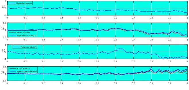
process.The curves in Figure 1 represents a trajectory of the approximate solution computed by the presented method with a trajectory of exact solution.

Example 2. Consider the following linear stochastic Volterra integral equation,

X(t) = 1

12+

Z t

0

cos(s)X(s)ds+

Z t

0

(15)

Figure 2. Simulation of Brownian motion are shown in graphs (a)

with J = 6 and (c) with J = 7. Graphs (b) and (d) show the

proposed analytical approximate and exact solutions of equation (6.1)

corresponding to the simulation of Brownian motion shown in (b) and (d) respectively.

0 0.1 0.2 0.3 0.4 0.5 0.6 0.7 0.8 0.9 1

(a)

-2 0 2

Brownian Motion

0 0.1 0.2 0.3 0.4 0.5 0.6 0.7 0.8 0.9 1

(b)

0.5 1 1.5

Exact Solution Approximate Solution

0 0.1 0.2 0.3 0.4 0.5 0.6 0.7 0.8 0.9 1

(c)

-1 0 1

Brownian Motion

0 0.1 0.2 0.3 0.4 0.5 0.6 0.7 0.8 0.9 1

(d)

0.5 1 1.5

with the exact solution X(t) = 1

12e

−t

4+sin(t)+ sin(2t)

8 + Rt

0sin(s)dB(s) where X(t) is an

unknown stochastic process defined on the probability space (Ω, z, P), and B(t) is

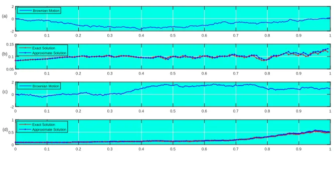
a Brownian motion process.The curves in Figure 2 represents a trajectory of the approximate solution computed by the presented method with a trajectory of exact solution.

6.1. Application to general stock model. The market consists of a riskless cash

bond,{A(t)}t≥0, and a single risky asset with price process {S(t)}t≥0 governed by

dAt=rtAtdt, A0= 1,

dSt=µtStdt+σtStdBt, (6.3)

where{W(t)}t≥0is aP-Brownian motion generating the filtration{F }t≥0and{r(t)}t≥0,

{µ(t)}t≥0and{σ(t)}t≥0are{F }t≥0-adapted processes. Evidently, a solution to these

equations should take the form

   

  

At=exp Z t

0 rudu

,

St=S0exp Z t

0

µu−

1

2σ

2 u

du+

Z t

0

σudBu

.

(16)

0 0.1 0.2 0.3 0.4 0.5 0.6 0.7 0.8 0.9 1

(a)

-2 0 2

Brownian Motion

0 0.1 0.2 0.3 0.4 0.5 0.6 0.7 0.8 0.9 1

(b)

0.05 0.1 0.15

0 0.1 0.2 0.3 0.4 0.5 0.6 0.7 0.8 0.9 1

(c)

-2 0 2

Brownian Motion

0 0.1 0.2 0.3 0.4 0.5 0.6 0.7 0.8 0.9 1

(d)

0 0.5 1

For example, consider the following general stock model,

   

  

dAu= sin(u)Audu, B0= 1, u∈[0,1),

St= 1

10 +

Z t

0

ln(1 +u)Sudu+

Z t

0

uSudBu, u, t∈[0,1),

(6.5)

with the exact solution At = e1−cos(t) and St = ₁₀1e(1+t) ln(1+t)−t−t

3 6+

Rt

0udBu_{, for}

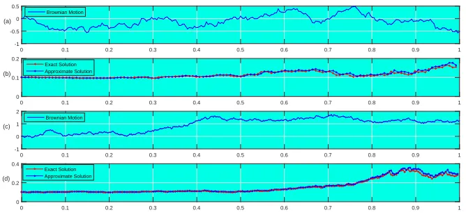
0 ≤ t < 1. Figure 4 shows two trajectory of the analytical approximate solution computed by the presented method with the trajectory of the exact solutions for

levelsJ= 6 and J = 7.

Theorem 6.1. Let Wt, t≥0 be a Brownian motion, and let ∆(t) be a nonrandom function of time. Define I(t) =Rt

0∆(u)dBu. For t≥0, the random variable I(t) is normally distributed with expected value zero and varianceRt

0∆ 2₍_u₎_du_.

Proof. See [19].

Corollary 6.2. Theorem (6.1) implies that the random variables lnX(t) in exam-ples (6.1) and (6.2) and lnSt in example (6.5) are normally distributed. Therefore, confidence intervals for these random variables and thereafter forX(t)andStcan be obtained. As an special case, we have

lnSt∼ N

ln 1

10 + (1 +t) ln(1 +t)−t−

t3

6,

t2

2

(17)

0 0.1 0.2 0.3 0.4 0.5 0.6 0.7 0.8 0.9 1

(a)

-1 -0.5 0 0.5

Brownian Motion

0 0.1 0.2 0.3 0.4 0.5 0.6 0.7 0.8 0.9 1

(b)

0 0.1 0.2

0 0.1 0.2 0.3 0.4 0.5 0.6 0.7 0.8 0.9 1

(c)

-1 0 1 2

Brownian Motion

0 0.1 0.2 0.3 0.4 0.5 0.6 0.7 0.8 0.9 1

(d)

0 0.2 0.4

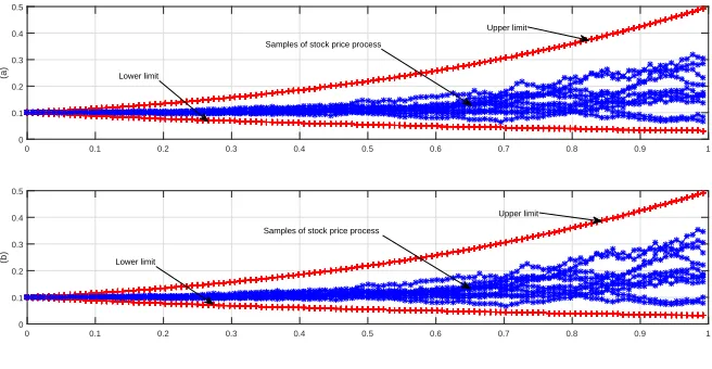
Figure5shows a 95% confidence region for the stock price process, in Figure5-(a)

100 sample paths for the exact solutionSt = ₁₀1e(1+t) ln(1+t)−t−t3

6+ Rt

0udBu with the

upper and lower limits corresponding to the 95% confidence region is shown where,

Figure5-(b) shows the approximate sample paths corresponding to 100 sample paths

of the exact solution and the 95% confidence region.

7. _Conclusion

Mail goal of the presented work has been to construct an approximation to the solu-tion of stochastic Volterra integral equasolu-tions. In the above discussion, the collocasolu-tion points with Haar wavelets, which have the property of orthogonality, is employed to achieve this goal. Using the new method for finding the Haar wavelet coefficients enables us to reduce the computation costs. There is a good agreement between ob-tained results and exact values that demonstrate the validity of the present method for this type of problems and gives the method a wider applicability. The method also applied to general stock model and the obtained results showed the ability and the accuracy of the method.

Acknowledgment

(18)

Figure 5. The 95% confidence region for the general stock model;

Figure (a) shows the sample paths obtained from the exact solution where Figure (b) shows the sample paths obtained from the proposed method.

0 0.1 0.2 0.3 0.4 0.5 0.6 0.7 0.8 0.9 1

(a)

0 0.1 0.2 0.3 0.4 0.5

0 0.1 0.2 0.3 0.4 0.5 0.6 0.7 0.8 0.9 1

(b)

0 0.1 0.2 0.3 0.4 0.5

Lower limit

Upper limit

Samples of stock price process

Lower limit

Samples of stock price process

Upper limit

References

[1] Z. Abbas, S. Vahdati, K. A. Atan, and N. M. A. N. Long, Legendre

multi-wavelets direct method for linear integro-differential equations, Appl. Math. Sci.,

3(14)(2009), 693–700.

[2] Z. Abbas, S. Vahdati, and M. Ghasemi, Legendre multi-wavelets direct method

for solving fredholm integral equations of the second kind, Aust. J. Basic Appl.

Sci., 4(9)(2010), 4193–4199.

[3] I. Aziz and Siraj-ul-Islam,New algorithms for the numerical solution of nonlinear

fredholm and volterra integral equations using Haar wavelets, J. Comput. Appl.

Math.,239(2013), 333–345.

[4] R. F. Bass,Stochastic Processes, Cambridge University Press, 2011.

[5] A. Boggess and F. J. Narcowich,A First Course in Wavelets with Fourier

Anal-ysis, Prentice Hall, 2001.

[6] C. Chen and C. Hsiao,Haar wavelet method for solving lumped and

distributed-parameter systems, IEE Proc. Control Theory Appl.,144(1)(1997), 87–94.

[7] S. Jankovic and D. Ilic,One linear analytic approximation for stochastic

integro-differential equations, Acta, Math. Sci.,30 (2010), 1073–1085.

[8] Y. Khan, M. Ghasemi, S. Vahdati, and M. Fardi,Legendre multi-wavelets to solve

oscillating magnetic fields integro-differential equations, U.P.B. Sci. Bull., Series A, 76(1)(2014), 51–58.

[9] M. Khodabin, K. Maleknejad, M. Rostami, and M. Nouri, Numerical solution

(19)

Comput. Model., 53(9)(2011), 1910–1920.

[10] M. Khodabin, K. Maleknejad, M. Rostami, and M. Nouri, Interpolation

solu-tion in generalized stochastic exponential populasolu-tion growth model, Appl. Math.

Model.,36(3)(2012), 1023–1033.

[11] M. Khodabin, K. Maleknejad, M. Rostami, and M. Nouri,Numerical approach

for solving stochastic volterra-fredholm integral equations by stochastic opera-tional matrix, Comput. Math. Appl.,64(6) (2012), 1903–1913.

[12] U. Lepik and E. Tamme.Application of the Haar wavelets for solution of linear

integral equations, Dyn. Syst. Appl, Proc., (July, Antalya, Turkey), (2004), 494– 507.

[13] U .LepikandE.Tamme.Solution of nonlinear fredholm integral equations via the

haar wavelet method, Proc. Est. Acad. Scie. Phy. Math., (2017), 17–27.

[14] K. Maleknejad, M. Khodabin, and M. Rostami.A numerical method for solving

m-dimensional stochastic ito-volterra integral equations by stochastic opera-tional matrix, Comput. Math. Appl.,63(1) (2012), 133–143.

[15] K. Maleknejad, M. Khodabin, and M. Rostami.Numerical solution of stochastic

volterra integral equations by a stochastic operational matrix based on block pulse functions, Math. Compt. Model.,55(3) (2012), 791–800.

[16] K. Maleknejad and F. Mirzaee.Numerical solution of stochastic linear heat

con-duction problem by using new algorithms, Appl. Math. Comput., 163(1)(2005), 97–106.

[17] T. Mikosch.Elementary Stochastic Calculus with Finance in view, World

Scien-tific, 1998.

[18] U. Saeed and M. ur Rehman.Haar wavelet operational matrix method for

frac-tional oscillation equations, Int. J. of Math. Math. Sci., 2014(2014).

[19] E. Shreve Steven.Stochastic Calculus for Finance II: Continuous-Time Models,

Springer, 2004.

[20] Siraj-ul-Islam, Imran Aziz, A. S. Al–Fhaid,An improved method based on Haar

wavelets for numerical solution of nonlinear integral and integro- differential equations of first and higher orders, J. Comput. Appl. Math., 260(2014), 449– 469.

[21] Siraj-ul-Islam, I. Aziz, Fazal Haq,A comparative study of numerical integration

based on Haar wavelets and hybrid functions, Comput. Math. Appl.,59(6)(2010), 2026–2036.

[22] H. A. Zedan and E. Alaidarous,Haar wavelet method for the system of integral

equations, Abstr. Appl. Anal.,2014(2014).

[23] H. Zhang, C. Zhu, X. Su, and X. Nie,A stable hankel transforms algorithm based

on Haar wavelet decomposition for noisy data, Math. Prob. Eng.,2015(2015).

[24] X. Zhang, Euler schemes and large deviations for stochastic volterra equations

with singular kernels, J. Differ. Equ.,44(2008), 2226– 2250.

[25] X. Zhang, Stochastic volterra equations in banach spaces and stochastic partial