Stable Gaussian radial basis function method for solving Helmholtz equations

Stable Gaussian radial basis function method for solving Helmholtz

equations

Jalil Rashidinia∗

School of Mathematics, Iran University of Science and Technology, Tehran, Iran.

E-mail: [email protected]

Manoochehr Khasi

School of Mathematics, Iran University of Science and Technology, Tehran, Iran.

E-mail: m [email protected]

Abstract Radial basis functions (RBFs) are a powerful method for obtaining the numerical solution of high-dimensional problems. They are often referred to as a meshfree method and the spectrally accurate can be achieved by them. In this paper, we ana-lyze a new stable method for evaluating Gaussian radial basis function interpolants based on the eigenfunction expansion. We develop our approach in two-dimensional spaces for solving Helmholtz equations. In this paper, the eigenfunction expansions are rebuilt based on Chebyshev polynomials which are more suitable in numerical computations. Numerical examples are presented to demonstrate the effectiveness and robustness of the proposed method for solving two-dimensional Helmholtz equa-tions.

Keywords. Gaussian radial basis functions, Eigenfunction expansion, Helmholtz equations, Sylvester

sys-tem.

2010 Mathematics Subject Classification. 65M99, 65N99, 76R50.

1. _Introduction

Helmholtz equation is very important in a variety of science and engineering prob-lems, for example, in physics, technology, geophysics and optical problems. There are several numerical methods for solving the Helmholtz equation. Among them we can mention the Finite element method in [2], the Finite volume method in [13,21], the Boundary element method in [22], spectral element methods in [17,19], radial basis function method in [15], or spectral methods in [1,16].

Radial basis functions (RBFs) have been used in many branches of science and engineering. Today there are many books related to the theory, applications and implementations of RBFs (see [3,6,23,25]). By using infinitely smooth basis functions such as Gaussians or Multiquadric , the exponential convergence rate can be achieved [9,25]. The best accuracy can usually be obtained when the shape parameter is small. But we should mention that as the shape parameter becomes small, the interpolant

Received: 17 September 2017 ; Accepted: 27 October 2018.

∗Corresponding author.

matrix becomes increasingly ill-conditioned. This fact has led to a growing number of stable approaches to overcome this problem, such as the Contour-Pad´e approach [8] or the RBF-QR method which in 2007 was introduced by Fornberg and Piret [10, 11] and later on by Larsson [14]. In [7], Fasshauer and McCourt developed a different type of the RBF-QR method by considering an eigenfunction expansion of the Gaussian RBF. They established a connection between the RBF-QR algorithm and Mercer’s theorem which states any positive definite kernel such as Gaussian has an eigenfunction expansion . In our previous work [20], we changed the eigenfunction expansion approach for evaluating Gaussian RBF interpolants by taking advantage of the orthogonality of the eigenfunctions which are based on Hermite polynomials.

In this article, we study numerical solution by a stable approach based on the eigenfunction expansions of Gaussian Radial basis functions which is an extension of our previous work [20]. The eigenfunction expansions are rebuilt based on Chebyshev polynomials, which are more suitable in numerical computations.

In this paper, we consider the following two-dimensional Helmholtz equation

∆u+k2u=f(x, y), in Ω, (1.1)

wheref is a smooth functions, ∆ = _∂x∂22 + ∂2

∂y2 is Laplacin operator, Ω is a bounded

domain in_R2_{,k is the wavenumber defined as k:= 2πp/v withpand v stating} fre-quency and speed, respectively, anduis the unknown solution representing a pressure field. The wavenumberkis a constant for the homogeneous medium, and varies for the heterogeneous medium. On the boundary ∂Ω, a Robin boundary condition is used:

αu(x, y) +β∂u

∂n(x, y) =h(x, y), on ∂Ω, (1.2)

where n is the outward unit normal vector to the boundary, h(x, y) is a smooth function, and α, β are non zero, simultaneously. If α 6= 0, β = 0, the boundary conditions can be imposed as Dirichlet boundary conditions and ifα= 0,β 6= 0, they can be imposed as Neumann boundary conditions.

The remaining part of this paper is organized as follows. Section 2 is devoted to some essential concepts about the stable method for Gaussian RBF interpolation based on eigenfunction expansions. In Section 3, the solution of two-dimensional Helmholtz equations are investigated. In Section 4, some numerical experiments that illustrate the accuracy, efficiency and stability of the proposed method are included.

2. _{A new stable method for 2d Gaussian RBF interpolation} Before discussing the discretization of the equation (1.1), we present a brief sum-mary of the new stable method for Gaussian RBF interpolation. Based on Mercer’s theorem, every positive definite kernelK: Ω×Ω→_Rwhere Ω⊂_Rd_{, can be explained}

in terms of the positive eigenvaluesλn →0 and normalized eigenfunctions ϕn of an

associated compact integral operator [24]. In fact

K(x,z) =

∞

X

n=1

Now supposeK is a native Hilbert space of functions on Ω, X={x1, . . . ,xN} ⊂ Ω

is the set of centers andKX = span{K(·,xj), xj ∈X} is the subspace spanned by

the basisK(·,xj), 1≤xj ≤N. We can write the interpolantsf ∈ KX off ∈ Kat

x1, . . . ,xN as

sf(x) = N

X

j=1

cjK(x,xj),

where the coefficients cj are determined by the interpolation conditions sf(xj) =

f(xj) : j = 1,· · · , N; i.e., they can be obtained by solving the following N ×N

linear system

Kc=f,

wheref = (f(x1),· · · , f(xN))T,c= (c1,· · ·, cN)T, and

K= 

 

K(x1,x1) · · · K(x1,xN)

..

. ...

K(xN,x1) · · · K(xN,xN)



 .

In applications, we have to truncate the series in (2.1). By choosingN terms of the series (2.1), and ignoring the truncation error, we can approximate the kernel as

K(x,xj) = N

X

n=1

λnϕn(x)ϕn(xj).

Therefore the interpolants_f becomes

s_f(x) =

N

X

j=1

cj N

X

n=1

λnϕn(x)ϕn(xj) =VTΦ(x)ΛN ΦXc,

whereVT

Φ(x) = (ϕ1(x), . . . , ϕN(x)),

ΛN =



 

λ1 0

. ._.

0 λN





, and ΦX= 

 

ϕ1(x1) · · · ϕ1(xN)

..

. ...

ϕN(x1) · · · ϕN(xN)



 .

In the same manner as in [4,20], we can show that

s_f(x) =VT_Φ(x)Φ−T_X f. (2.2)

For small values of the Gaussian shape parameterε, the eigenvaluesλn decrease

to-ward zero [18] rapidly, and this causes the system to become ill-conditioned. So that

ΛN, which depends on eigenvalues, is eliminated. We can conclude that one of the

source of ill-conditioning is removed.

We consider the one-dimensional Gaussian RBF, which is a positive definite kernel. Based on Mercer’s theorem

e−ε2(x−z)2=

∞

X

n=1

where the ϕn are orthogonal functions with respect to the weight function ρ(x) = α

√ πe

−α2_x2

,

ϕn(x) =

p

βe−δ2x2Hen−1(αβx), (2.3)

andHen(x) are normalized Hermite polynomials (see [7,20]). Also

β =

1 +4ε 2

α2 14

, δ2=α 2

2 (β 2_−1),

and the eigenvaluesλn are given by

λn=

r

α2

α2_+ε2_+δ2

_ε2

α2_+ε2_+δ2 n−1

, n= 1,2, . . . .

By using (2.3), the vector functionVΦ(x) and the matrixΦX can be decomposed as

VΦ(x) = p

β e−δ2x2 VH(x), (2.4)

and

ΦX=

p

β HX DX, (2.5)

where

VH(x) =



 

e

H0(αβx) .. .

e

HN−1(αβx) 



, HX = 

 

e

H0(αβx1) · · · He0(αβxN)

..

. ...

e

HN−1(αβx1) · · · HeN−1(αβxN)



 ,

and

DX =



 

e−δ2x2_{1 0}

. ._.

0 e−δ2x2_N



 .

Since the Hermite polynomials values can grow dramatically, the algorithm for eval-uation of Gaussian RBFs can become unstable. Therefore in the following we show that the eigenfunctions can be rebuilt according to any other orthogonal polynomi-als, like Chebyshev polynomipolynomi-als, which are more stable for numerical computation. Let{pn(x)}∞n=0 be a family of polynomials, since {p0,· · ·, pn} is a basis forπn (the

space of all polynomials of degree at mostn), Hen(αβx) can be presented as a linear

combination of its members as follows:

e

Hn(αβx) = n

X

k=0

cn,kpk(x), (2.6)

so      e

H0(αβx)

e

H1(αβx) .. .

e

H_N−1(αβx)      =      c₀₀

c₁₀ c₁₁ 0 ..

. ... . ..

c_N−1,0 c_N−1,1 · · · c_N−1,N−1

         

p0(x)

p1(x) .. .

The above formula can be written in matrix-vector form asVH(x) =C Vp(x) and

consequentlyHX=C PX where

PX=



 

p0(x1) · · · p0(xN)

..

. ...

p_N−1(x1) · · · pN−1(xN)



 ,

is a polynomial Vandermonde-type matrix [5,12].

Therefore, from the relations (2.2), (2.4), and (2.5), we have

s_f(x) = pβ e−δ2x2 VT_H(x) √1 βH

−T

X D

−1

X f

= e−δ2x2 VpT(x)C T

C−T P−T_X D−_X1 f

= e−δ2x2 V_pT(x)P−T_X D−_X1 f,

so we rebuild eigenfunctions according topn(x), consequently we rebuildϕn(x) as

ϕn(x) =

p

βe−δ2x2pn−1(x).

Now we can generalize the above discussion for two-dimensional interpolation for-mula forf : [a, b]×[c, d]→R. LetY ={y1,· · ·, yM}be a set of arbitrary grid points

on [c, d] and ¯Ω :=X×Y ={(xi, yj) : i= 1,2,· · ·, N, j= 1,2,· · · , M}be the tensor

product grid points on [a, b]×[c, d]. By using the tensor product form of the Gaussian kernel, we have

sf(x, y) = N

X

j=1

cj N

X

n=1

M

X

m=1

λmλnϕn(x)ϕn(xj)ϕm(y)ϕm(yj),

where

ϕm(y) =

p

β e−δ2y2pm−1(x), m= 1,· · ·, M, y∈[c, d].

Just as in [20], we can show that

sf(x, y) =VTΦ(x)Φ−TX F Φ −1

Y VΦ(y), (2.7)

where

F= 

 

f(x1, y1) · · · f(x1, yM) ..

. ...

f(xN, y1) · · · f(xN, yM) 

 .

Similarly, by using (2.4) and (2.5), we can decomposeVΦ(y) andΦY as

VΦ(y) = p

β e−δ2y2VP(y),

and

ΦY =

p

By these decompositions, the formula (2.7) can be obtained as:

sf(x, y) = e−δ 2_(x2_+y2₎

VT_P(x)P−T_X F P¯ −_Y1 VP(y), (2.8)

whereF¯=D−_X1 F D−_Y1.

Remark 1. Up until now the polynomials pn were arbitrary. In particular we can, use Chebyshev polynomials (also shifted Chebyshev polynomials) instead of Hermite

polynomials. Therefore, in this paper, when we approximatef : [a, b]→Rby Gaussian

RBFs, theϕn(x)’s are modified as

ϕn(x) =

p

β e−δ2x2Tbn−1(α1x+α2), x∈[a, b],

where

b

Tn(x) =

  

 

2

√

N, n= 0,

q 2

NTn(x), n≥1,

and the parametersα1, α2, which control the Chebyshev polynomials, can be chosen

arbitrary. While if we choose α1 = _b−a2 , α2 = −a_b−a+b, then the shifted Chebyshev

polynomials become bounded such that|Tn(α1 x+α2)| ≤1 forx∈[a, b].

3. _{Implementation of the method}

In this section, we want to solve two dimensional Helmholtz equation (1.1) on Ω = [a, b]×[c, d] by a collocation method based on Gaussian eigenfunctions. The boundary conditions (1.2) can be considered as

         

        

α1u(a, y) +β1ux(a, y) =h1(a, y),

α2u(b, y) +β2ux(b, y) =h2(b, y),

α3u(x, c) +β3uy(x, c) =h3(x, c),

α4u(x, d) +β4uy(x, d) =h4(x, d),

(3.1)

Suppose that the approximate solution of (1.1) is

U(x, y) =VTΦ(x)Φ−TX U Φ −1

Y VΦ(y), (3.2)

where [U]_ij =U(xi, yj). For solving the equation and illustrating the algorithm, it is

necessary to decompose and rearrange the matrixUas

U= 

     

u₁₁ u_1M u₁₂ · · · u_1,M−1

u_N,1 u_N,M u_N2 · · · u_N,M−1

u₂₁ u_2,M u₂₂ · · · u_2,M

..

. ... ... . .. ...

u_N−1,1 u_N−1,M u_N−1,2 · · · u_N−1,M−1



     

=

Ucor_B Urow_B Ucol

B UI

In fact, we decomposeU to four matrices Ucor_B ,U_Brow, Ucol_B ,UI which are the four

corners, the up and down boundaries, the left and right boundaries, and the interior entries ofU, respectively. We should mention that it is necessary to rearangement the other matrices in the formula (3.2) asU, to avoid deformation of that. For the Dirichlet boundary conditions, all of the entries along the boundary of the matrixU

are known, so it is necessary to obtain onlyUIby simplifying the equation with some

matrix algebraic operations. For the Neumann boundary conditions, the problem be-comes a little complicated.

Collocating the equation at the interior points and using the boundary data at the boundary points leads to the following system of equations

V_Φ00T(xi) Φ−TX U Φ −1

Y VΦ(yj) +V

T

Φ(xi)Φ−TX U Φ −1

Y V

00

Φ(yj)

+ k2U=f(xi, yj), (3.3)

for 1< i < N, 1< j < M, associated with boundary conditions

         

        

α1u(x1, yj) +β1ux(x1, yj) =h1(x1, yj),

α2u(xN, yj) +β2ux(xN, yj) =h2(xN, yj), i= 2,· · ·, N−1,

α3u(xi, y1) +β3uy(xi, y1) =h3(xi, y1),

α4u(xi, yM) +β4uy(xi, yM) =h4(xi, yM), j= 1,· · ·, M.

(3.4)

By denoting the following

e

ΨT_X = 

 

V_Φ00T(x2) .. .

V00_ΦT(xN−1)





, ΦeY =

VΦ(y2) · · · VΦ(yM−1)

,

andA= [aij] =ΨeT_X Φ−T_X , we consider the first term on the left-hand side of (3.3). In the same manner as in [20] we can show that

e

ΨT_X Φ−T_X U Φ−_Y1 ΦeY

= 

   

a1,1 a1,N

a2,1 a2,N

..

. ...

a_N−2,1 aN−2,N 

   

| {z }

=AB

u1,2 u1,3 · · · u1,M−1

u_N,2 u_N,3 · · · u_N,M−1

| {z }

+     

a1,2 · · · a1,N−1

a2,2 · · · a2,N−1 ..

. ...

aN−2,2 · · · aN−2,N−1 

   

| {z }

=AI



 

u2,2 u2,3 · · · u2,M−1 ..

. ... ...

u_N−1,2 uN−1,3 · · · uN−1,M−1



 

| {z }

=UI

. (3.5)

Using the first two boundary conditions, we have

α1 0 0 α2

| {z }

=α12





Urow₁

Urow_N



+

β1 0 0 β2

| {z }

=β12

˜

A U=

h1(x1, y1) · · · h1(x1, yM)

h2(xN, y1) · · · h2(xN, yM) , where ˜ A=  

V0_ΦT(x1)

V0_ΦT(x_N) 

 Φ−T_X .

therefore

α12 h

Ucor_B |Urow_B i+β12 A U˜ = h

Hcor|Hrowi.

Now by decomposing ˜AandU, we want to obtain Urow_B andUcor_B , in fact

˜

A U = _˜

AB A˜I

Ucor

B U˜rowB

Ucol

B UI

= A˜B UcorB +AI UBcol A˜BUrowB + ˜AI UI.

Now by using two above equations

α12U cor

B +β12

h ˜

AB UcorB + ˜AI UcolB

i

=Hcor,

and

α12U row

B +β12

h ˜

AB UrowB + ˜AI UI

i

=Hrow.

So by denotingK1=α12+β12A˜B, we have

Ucor_B =K−₁1hHcor−β12 A˜I UcolB

i

, (3.6)

and

Urow_B =K−₁1hHrow−β12 A˜I UI

i

. (3.7)

Now by denoting

e

ΦT_X= 

 

VT

Φ(x2) .. .

VT

Φ(xN−1)





, ΨeY =

V00_Φ(y2) · · · VΦ00(yM−1)

andB= [bij] =Φ−Y1ΨeY, we can similarly obtained

e

ΦT_X Φ−T_X U Φ−_Y1 ΨeY =



   

u2,1 u2,M

u3,1 u3,M

..

. ...

uN−1,1 uN−1,M



   

| {z }

=Ucol

B

b1,1 b1,2 · · · b1,M−2

bM,1 bM,2 · · · bM,M−2

| {z }

=BB

+ 

 

u2,2 u2,3 · · · u2,M−1 ..

. ... ...

uN−1,2 uN−1,3 · · · uN−1,M−1 

 

| {z }

=UI



 

b2,1 b2,2 · · · b2,M−2 ..

. ... ...

bM−1,1 bM−1,2 · · · bM−1,M−2 

 

| {z }

=BI

,(3.8)

and

Ucol_B =hHcol−UI B˜I β34 i

K−₂1, (3.9)

whereK2=α34+ ˜BB β34.

Now, by substituting (3.7) in (3.5), and (3.9) in (3.8), we obtain the following Sylvester system

A UI+UI B+C=0, (3.10)

where

A = AI+

k2 2 I,

B = BI+

k2

2 I,

C = AB GrowB +GcolB BB−Fe,

and [Fe]i,j=f(xi, yj), i= 2,· · ·, N, j= 2,· · · , M.

The equation (3.10) can be solved inMatlabby using the command sylvester, which first transforms theAandBmatrices to complex Schur form, then computes the solution of the resulting triangular system and finally transforms the solution back.

After solving (3.10),UI will be obtained (the solution in interior points), then by

using (3.7) and (3.9),Urow

B andUcolB will be obtained, and finally by using (3.6),UcorB

will be obtained. Also by using (3.2), we can obtain a closed form solution for the Helmholtz equation.

4. _{Numerical Results}

Table 1. The local and global error for different values of grid points

for Example 1.

N×M Uniform points Chebyshev points

Local error Global error Local error Global error

11×11 3.79×10−02 4.02×10−01 3.09×10−04 1.42×10−02

13×13 1.97×10−03 _1.72×10−02 _5.84×10−06 _2.99×10−05

15×15 5.14×10−05 _3.85×10−04 _6.20×10−08 _3.41×10−06

17×17 3.72×10−07 2.45×10−06 2.12×10−10 1.33×10−08

19×19 1.40×10−08 _7.98×10−08 _2.21×10−12 _1.03×10−10

21×21 3.25×10−09 _3.37×10−08 _1.38×10−13 _1.37×10−12

23×23 1.78×10−07 7.22×10−07 1.43×10−13 8.47×10−13

Intel(R) Core(TM) i5-4460 processor (3.20GHz CPU), a 64-bit Windows 7 operating system, and a 16 GB internal memory . In all examples, we usedε= 1,α= 1.9 and we used uniform grid points and Chebyshev collocation points.

The accuracy is measured by computing the local and global error of

ku−Uk

∞,Ω¯ = max|u(xi, yj)−Ui,j|

(xi,yj)∈Ω¯

,

and

ku−Uk

∞,Ω = max|u(x, y)−U(x, y)|

(x,y)∈Ω

,

where the second norm is approximated on 300×(b1−a1+b2−a2) evenly spaced points.

Example 1. Consider the following two-dimensional Helmholtz equation

 



∂2_u(x,y) ∂x2 +

∂2_u(x,y) ∂y2 + 9π

2_{u(x, y) =−9π}2_{sin(3πx) sin(3πy), (x, y)∈Ω}

u(x, y) = 0, (x, y)∈∂Ω

Figure 1. Error with the 17 ×17 uniform grid point (left) and

Chebyshev grid points (right) for Example 1.

0

0.5 1

0 0.5 1 0 0.2 0.4 0.6 0.8 1

x 10−6

absolute error

0

0.5

1

0 0.5 1 0 1 2 3 4

x 10−9

x y

absolute error

Example 2. Consider the following two-dimensional Helmholtz equation from [15]

     

    

∂2_u(x,y) ∂x2 +

∂2_u(x,y)

∂y2 + 2u(x, y) = 2x−4y, in Ω = [0,1]×[0,1]

uy(x, y) =h2(x, y), on Γ2= [0,1]× {0}

u(x, y) =h1(x, y), on Γ1=∂Ω\Γ2

where the exact solution is u(x, y) = sin(√3x) sinh(y) + cos(√2y) +x−2y, and

Table 2. The local and global error for different values of grid points

for Example 2.

N×M Uniform points Chebyshev points

Local error Global error Runtime Local error Global error Runtime

11×11 4.37×10−05 1.89×10−02 0.1824 1.34×10−04 1.74×10−03 0.1895

13×13 1.39×10−06 _4.12×10−04 _{0.1813 1.79×10}−06 _1.76×10−05 _0.1937

15×15 8.45×10−08 _1.09×10−05 _{0.1776 2.96×10}−08 _1.75×10−07 _0.1865

17×17 3.32×10−09 5.94×10−07 0.1779 4.94×10−10 3.37×10−09 0.1910

19×19 1.69×10−09 _2.06×10−08 _{0.1804 8.10×10}−12 _4.94×10−11 _0.1927

21×21 2.56×10−09 _9.37×10−09 _{0.1795 3.81×10}−13 _2.33×10−12 _0.1953

23×23 6.71×10−08 1.38×10−08 0.1875 1.43×10−12 8.68×10−12 0.1905

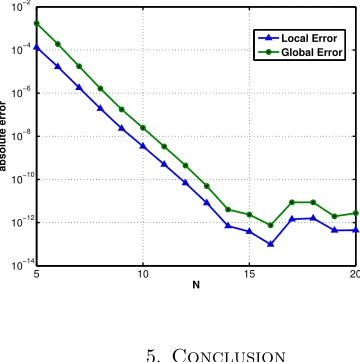
Figure 2. Absolute errors as function of N for Chebyshev grid

points for Example 2.

5 10 15 20

10−14 10−12 10−10 10−8 10−6 10−4 10−2

N

absolute error

Local Error Global Error

5. _Conclusion

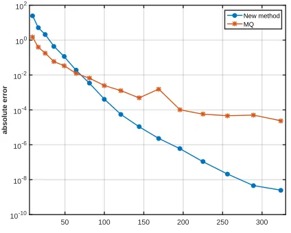
Figure 3. Absolute errors as function of N for Chebyshev grid

points for Example 2.

Number of grid points

50 100 150 200 250 300

absolute error

10-10 10-8 10-6 10-4 10-2 100 102

New method MQ

References

[1] K. Atkinson, O. Hansen, and D. Chien,A spectral method for elliptic equations: The Neumann problem, Adv. Comput. Math.,34(3) (2011), 295–317.

[2] I. Babuska, F. Ihlenburg, E. T. Paik, and S. A. Sauter, A generalized finite element method for solving the helmholtz equation in two dimensions with minimal pollution, Comput. Method. Appl. Mech. engg.,128(3-4) (1995), 325–359.

[3] M. D. Buhmann,Radial basis functions: theory and implementations, Cambridge university press,12(2003).

[4] R. Cavoretto, G. E. Fasshauer, and M. Mccourt,An introduction to the Hilbert-Schmidt SVD using iterated Brownian bridge kernels, Numer. Algor.,68(2) (2015), 393-422.

[5] J. Demmel and P. Koev,Accurate SVDs of polynomial Vandermonde matrices involving or-thonormal polynomials, Lin. Algeb. Applic.,417(2-3) (2006), 382–396.

[6] G. E. Fasshauer,Meshfree approximation methods with Matlab:(With CD-ROM), World Scien-tific Publishing Co Inc,6, (2007).

[7] G. E. Fasshauer and M. J. Mccourt,Gaussian radial basis function interpolants, SIAM J. Sc. Comput.,34(2) (2012), A737–A762.

[8] B. Fornberg and G. Wright,Stable computation of multiquadric interpolants for all values of the shape parameter, Comput. Math. Appli.,48(5) (2004), 853–867.

[10] B. Fornberg and C. Piret,A stable algorithm for flat radial basis functions on a sphere, SIAM J. Sc. Comput.,30(1) (2007), 60–80.

[11] B. Fornberg, E. Larsson, and N. Flyer,Stable computations with Gaussian radial basis functions, SIAM J. Sc. Comput.,33(2) (2011), 869–892.

[12] W. Gautschi,The condition of Vandermonde-like matrices involving orthogonal polynomials, Lin. Algeb. Appl.,52(1983), 293–300.

[13] A. Handloviˇcov´a and I. Rieˇcanov´a,Numerical solution to the complex 2D Helmholtz equation based on finite volume method with impedance boundary conditions, Open Phy.,14(1) (2016), 436–443.

[14] E. Larsson, E. Lehto, A. Heryudono, and B. Fornberg,Stable computation of differentiation matrices and scattered node stencils based on Gaussian radial basis functions, SIAM J. Sc. Comput.,35(4) (2013), A2096–A2119.

[15] , J. Lin, W. Chen, and K. Y. Sze,A new radial basis function for Helmholtz problems, Eng. Anal. Bound. Elem.,36(12) (2012), 1923–1930.

[16] P. Martinsson,A direct solver for variable coefficient elliptic PDEs discretized via a composite spectral collocation method, J. Comput. Phy.,242(2013), 460–479.

[17] A. T. Patera,A spectral element method for fluid dynamics: laminar flow in a channel expan-sion, J. Comput. Phy.,54(3) (1984), 468–488.

[18] M. Pazouki and R. Schaback,Bases for kernel-based spaces, J. Comput. Appl. Math.,236(4) (2011), 575–588.

[19] C. Pozrikidis,Introduction to finite and spectral element methods using MATLAB, CRC Press, 2005.

[20] J. Rashidinia, G. E. Fasshauer, and M. Khasi,A stable method for the evaluation of Gaussian radial basis function solutions of interpolation and collocation problems, Comput. Math. Appl.,

72(1) (2016), 178–193.

[21] I. Rieˇcanov´a,Finite volume method scheme for the solution of Helmholtz equation, Proceedings of Aplimat, 14-th Conference on Applied Mathematics, Institute of Mathematics and Physics, Faculty of Mechanical Engineering STU in Bratislava, 2015.

[22] S. A. Sauter and C. Schwab,Boundary element methods, Springer-Verlag, Berlin, 2010. [23] R. Schaback,A practical guide to radial basis functions,Electronic Resource,11, 2007. [24] E. Schmidt,Uber die Aufl¨¨ osung linearer Gleichungen mit unendlich vielen Unbekannten,