Chebyshev Spectral Collocation Method for Computing Nu-merical Solution of Telegraph Equation
M. Javidi
Faculty of Mathematical Sciences, University of Tabriz, Tabriz, Iran.
E-mail: mo [email protected]
Abstract In this paper, the Chebyshev spectral collocation for one-dimensional
lin-ear hyperbolic telegraph equation is presented. Chebyshev spectral colloca-tion method have become very useful in providing highly accurate solucolloca-tions to partial differential equations. A straightforward implementation of these methods involves the use of spectral differentiation matrices. Firstly, we trans-form telegraph equation to system of partial differential equations with initial condition. Using Chebyshev differentiation matrices yields a system of or-dinary differential equations. Secondly, we apply fourth order Runge-Kutta formula for the numerical integration of the system of ODEs. Numerical re-sults verified the high accuracy of the new method, and its competitive ability compared with other newly appeared methods.
Keywords. Chebyshev spectral collocation method, telegraph equation, numerical results,
Runge-Kutta formula.
2010 Mathematics Subject Classification. 65M70.
1. Introduction
Consider one dimensional linear hyperbolic telegraph equation:
∂2u ∂t2 + 2α
∂u ∂t +β
2u= ∂2u
∂x2 +f(x, t), (x, t)∈[0,1]×[0,1], α > β ≥0. (1.1)
with initial conditions
u(x,0) =f0(x),
∂u
∂t(x,0) =f1(x) (1.2)
and boundary conditions
u(0, t) =g0(t), u(1, t) =g1(t), t≥0. (1.3)
Telegraph equation is commonly used in the study of wave propagation of elec-tric signals in a cable transmission line and also in wave phenomena. Many researchers have used various numerical and analytical methods to solve the
Telegraph equation. Mohebbi and Dehaghan [19] studied high order compact solution to solve the telegraph equation. Gao and Chi [13] used unconditionally stable difference scheme for a one-space dimensional linear hyperbolic equa-tion. Saadatmandi and Dehghan [20] developed a numerical solution based on Chebyshev Tau method. The authors of [22] used Legendre multiwavelet Galerkin method for solving the hyperbolic telegraph equation. Dehghan and Ghesmati [10] developed a numerical approach based on the truly meshless local weakstrong (MLWS) methods to deal with the second order two-space-dimensional telegraph equation. To solve the telegraph equation using the MLWS method, the conventional moving least squares (MLS) approximation is exploited in order to interpolate the solution of the equation. A time step-ping scheme is employed to approximate the time derivative. Das and Gupta [9] used homotopy analysis method for solving fractional hyperbolic partial differential equations. By using initial values, the explicit solutions of tele-graph equation for different particular cases have been derived. Abdou [1] used Adomian decomposition method for solving the telegraph equation in charged particle transport. The Authors of [15] developed a numerical tech-nique for the solution of second order one dimensional linear hyperbolic equa-tion. The method consists of expanding the required approximate solution as the elements of interpolating scaling functions. In their technique, by using the operational matrix of derivatives , they reduced the problem to a set of algebraic equations. Mohanty [17,18] made investigations on the one-space-dimensional hyperbolic equations.
approximate solution of an equation. In this paper we use Chebyshev spectral collocation method (CSCM) to solve Eq. (1.1) with the initial and boundary conditions (1.2)-(1.3).
The outline of this paper is as follows. Section 1 contains a brief summary on telegraph equation. In section 2, we review some of the standard facts on Chebyshev spectral collocation method. In the third section, we develop the theory of transformation of telegraph equation to system of ordinary differen-tial equations. In section 4, the numerical results of applying the method of this article on some test problems for the Eq. (1.1) are presented.
2. Chebyshev spectral collocation method
Consider a one-dimentional domain: −1 ≤ x ≤1. The domain of interest is discretized using the Gauss-Lobbato points defined as
{ξj}={cos( jπ
N)} N
j=0. (2.1)
We interpolateu(x) by the polynomialP(x) of degree at most N of the form:
P(x) =
N ∑
j=0
χj(x)u(ξj), (2.2)
in the Chebyshev-Gauss-Lobbato (C-G-L) points with χj(x) for j = 0(1)N,
are polynomial of degree at mostN such that
χj(ξk) =δjk, j, k= 0(1)N. (2.3)
It can be shown that (see [2,3,6,7,8,21]):
χj(x) =
(−1)j+1(1−x2)TN′ (x)
γjN2(x−ξ
j)
, j= 0(1)N, (2.4)
where
γ0 =γN = 2, γj = 1, j= 1(1)N−1,
andTN(x) the Chebyshev polynomial, i.e.,
TN(x) = cos(Narccosx). (2.5)
The values of derivative ddxkPk, with k= 1,2,· · · , p at the C-G-L points can be
computed by
d dkP
dxk =M
whereb. labels vector, e.g., Pb = (P(ξ0), P(ξ1),· · · , P(ξN))T and M(1) are the
differentiation matrices. The entries ofM(M(1)) are
mkj =− γk
2γj
(−1)j+k
sin((k+j)2πN) sin((k−j)2πN), k̸=j, 0≤k, j≤N, (2.7)
mkj =−
1 2cos(
kπ
N )(1 + cot
2(kπ
N )),k=j, k̸= 0, N, (2.8)
m00=−mN N =
2N2+ 1
6 . (2.9)
As an alternative approach, the diagonal entries ofM can be computed in the way that represents exactly the derivative of a constant [21]
mii=− N ∑
j=0,j̸=i mij.
3. CSCM for telegraph equation
In this section, we outline the main step of our method to solve the telegraph equation (1.1) with initial conditions (1.2) and boundary conditions (1.3) by using CSCM. Set ∂u∂t(x, t) =v(x, t).Then we can rewrite (1) as follows
∂v
∂t(x, t) =−2αv(x, t)−β2u(x, t) + ∂2u
∂x2(x, t) +f(x, t)
∂u
∂t(x, t) =v(x, t)
(3.1)
with the initial conditions
u(x,0) =f0(x), v(x,0) =f1(x) (3.2)
and the boundary conditions
u(0, t) =g0(t), u(1, t) =g1(t). (3.3)
Now we describe the Chebyshev pseudospectral method for system of PDEs (3.1)-(3.3) to convert it to system of ODEs. For this letN be a nonnegative integer and denote by δj = 12(1 +ξj), j = 0(1)N, the
Chebyshev-Gauss-Lobatto points in the interval [0,1]. We discretize (3.1) in space by the method of lines replacing ∂u∂x(δi, t),∂
2u
∂x2(δi, t) by pseudospectral approximations given by
∂ uk
∂xk(δi, t)≈2 N ∑
j=0
and Here M(k) is differentiation matrix of order k. Substituting (3.4) into (3.3) and taking into account that
u(δN, t) =g0(t),
u(δ0, t) =g1(t)), (3.5)
we obtain the following system of ODEs:
∂v
∂t(δi, t) =−2αv(δi, t)−β2u(δi, t)
+2∑Nj=1−1m2iju(δj, t) + 2(m2i0g1(t) +m2iNg0(t)) +f(δi, t), ∂u
∂t(δi, t) =v(δi, t), i= 1(1)N −1
(3.6)
with the initial conditions
u(δi,0) =f0(δi), v(δi,0) =f1(δi), i= 1(1)N −1. (3.7)
We can write the equations (3.6)-(3.7) in the matrix form as follows
dU
dt =AU +G, (3.8)
where U = [ U V ] , A=
[
oN−1,N−1 IN−1,N−1
B C
] , G=
[
oN−1,1
D ] , U =
u(δ1, t)
u(δ2, t) .. .
u(δN−1, t)
, V =
v(δ1, t)
v(δ2, t) .. .
v(δN−1, t)
, and B =
2(m211−β2) 2m212 . . . 2m21,N−1
2m221 2(m222−β2) . . . 2m22,N−1
..
. ... ...
2m2N−1,1 2m2N−1,2 . . . 2(m2N−1,N−1−β2)
N−1,N−1
, and C =
−2α 0 . . . 0 0 −2α . . . 0
..
. ... ...
0 0 . . . −2α
N−1,N−1
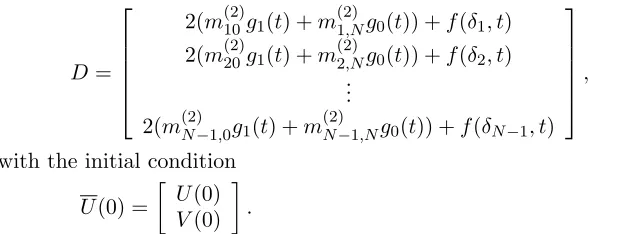
D=
2(m(2)10g1(t) +m(2)1,Ng0(t)) +f(δ1, t)
2(m(2)20g1(t) +m(2)2,Ng0(t)) +f(δ2, t) ..
.
2(m(2)N−1,0g1(t) +m(2)N−1,Ng0(t)) +f(δN−1, t)
,
with the initial condition
U(0) =
[ U(0)
V(0)
]
. (3.9)
We apply fourth order Runge-Kutta formula for the numerical integration of the system of ODEs (3.8) with initial conditions (3.9).
4. Numerical results
Example 1. We consider the Eq. (1.1) with the following conditions [1]:
f0(x) = sinh(x),
f1(x) =−2 sinh(x),
g0(t) = 0,
g1(t) =e−2tsinh(1),
f(x, t) = (3−4α+β2)e−2tsinh(x).
(4.1)
The exact solution is given by
u(x, t) =e−2tsinh(x). (4.2)
In this section, we give some computational results numerical experiments with the method based on the preceding sections. To show the efficiency of the present method for our problems in comparison with the exact solution we calculate the maximum error ||u||∞ defined by
||u||∞= max{|unumer−uexact|: 0≤i≤N}.
Where unumer and uexact are the numerical and exact solution, respectively.
Numerical computations were carried out in Matlab.
Table 1 show the absolute error using the technique presented in the previous section with ∆t= 0.001, N = 16, α= 20 and β= 10 for t= 0.5,1,1.5,2.
Table 1. Absolute error for u(δj, t) with ∆t = 0.001, N = 16, α = 20 and β = 10
fort= 0.5,1,1.5,2.
δ/t 0.5 1 1.5 2
δ2 0.0020 9.7848e−4 4.0835e−4 1.6057e−4
δ6 0.0024 0.0015 7.3220e−4 3.1182e−4
δ10 9.8950e−4 6.4268e−4 3.0918e−4 1.3295e−4
In Fig. 1, we plot exact solution and numerical solution at t = 1, N = 128, β = 10, α= 20 and ∆t= 0.001 for Example 1.
0 0.1 0.2 0.3 0.4 0.5 0.6 0.7 0.8 0.9 1 −0.02
0 0.02 0.04 0.06 0.08 0.1 0.12 0.14 0.16
x
u
Exact Approx
Figure 1. Exact solution and numerical solution att= 1, N= 128, β= 10, α= 20 and ∆t= 0.001 for Example 1.
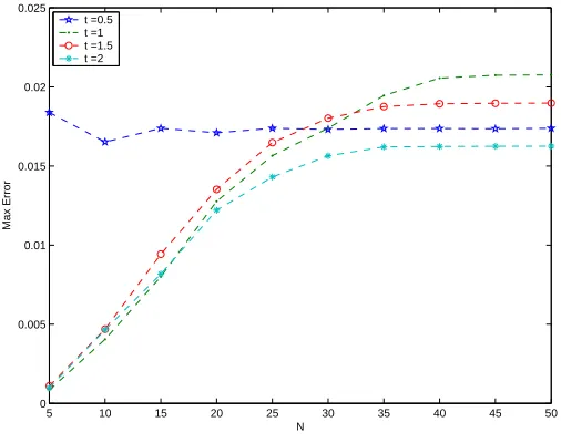
In Fig. 2, we plot max error at t = 0.5(0.5)2, N = 5(5)50, β = 1, α = 5 and ∆t= 0.001 for Example 1.
5 10 15 20 25 30 35 40 45 50
0 0.005 0.01 0.015 0.02 0.025
N
Max Error
t =0.5 t =1 t =1.5 t =2
In Fig. 3, we plot max error at t = 1, N = 5(5)50, β = 1 and ∆t = 0.001 for Example 1.
5 10 15 20 25 30 35 40 45 50
0 0.005 0.01 0.015 0.02 0.025
N
Max Error
α =5
α =10
α =15
α =20
Figure 3. Max error att= 1, N = 5(5)50, β = 1 and ∆t= 0.001 for Example 1.
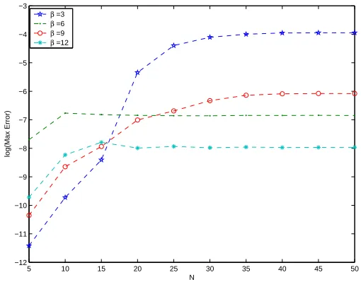
In Fig. 4, we plot log(max error) att= 1, N = 5(5)50, α= 2 and ∆t= 0.001 for Example 1.
5 10 15 20 25 30 35 40 45 50
−12 −11 −10 −9 −8 −7 −6 −5 −4 −3
N
log(Max Error)
β =3
β =6
β =9
β =12
In Fig. 5, we plot log(absolute error) att= 1, N = 16, α = 2 and ∆t= 0.001 for Example 1.
0 0.1 0.2 0.3 0.4 0.5 0.6 0.7 0.8 0.9 1 −14
−13 −12 −11 −10 −9 −8 −7 −6 −5
x
log(Absolute Error)
β =5
β =10
β =15
β =20
Figure 5. log(absolute error) att= 1, N = 16, α= 2 and ∆t= 0.001 for Example 1.
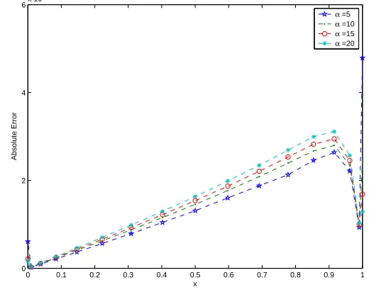
0 0.1 0.2 0.3 0.4 0.5 0.6 0.7 0.8 0.9 1 0
2 4 6x 10
−4
x
Absolute Error
α =5
α =10
α =15
α =20
Figure 6. Absolute error att= 1, N = 16, β= 20 and ∆t= 0.001 for Example 1.
Example 2. We consider the Eq. (1.1) with the following conditions:
f0(x) = sin(x),
f1(x) = 0,
g0(t) = 0,
g1(t) = cos(t) sinh(1),
f(x, t) =−2αsin(t) sin(x) +β2) cos(t) sin(x).
(4.3)
The exact solution is given by
u(x, t) = cos(t) sin(x). (4.4)
Table 2 show the absolute error using the technique presented in the pre-vious section with ∆t= 0.001, N = 16, α= 20 andβ = 10 at t= 0.5,1,1.5,2 for Example 2.
Table 2. Absolute error foru(δj, t) with ∆t= 0.0001, N = 64, α= 20 andβ = 10 at
t= 0.5,1,1.5,2 for Example 2.
δ/t 0.5 1 1.5 2
δ2 2.3747e−4 1.8608e−4 7.0089e−5 6.6330e−5
δ6 0.0017 0.0014 5.8266e−4 4.1998e−4
δ10 0.0032 0.0028 0.0013 6.0133e−4
δ14 0.0038 0.0036 0.0019 4.9635e−4
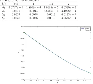
0 0.1 0.2 0.3 0.4 0.5 0.6 0.7 0.8 0.9 1 −0.4
−0.35 −0.3 −0.25 −0.2 −0.15 −0.1 −0.05 0 0.05
x
u
Exact Approx
Figure 7. Exact solution and numerical solution att= 2, N = 64, β= 10, α= 20 and ∆t= 0.0001 for Example 2.
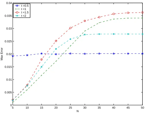
5 10 15 20 25 30 35 40 45 50 0
0.005 0.01 0.015 0.02 0.025 0.03 0.035 0.04
N
Max Error
t =0.5 t =1 t =1.5 t =2
Figure 8. Max error at t= 0.5(0.5)2, N = 5(5)50, β = 1, α= 5 and ∆t= 0.001 for Example 2.
In Fig. 9, we plot max error at t = 1, N = 5(5)50, β = 1 and ∆t = 0.001 for Example 2.
5 10 15 20 25 30 35 40 45 50
0 0.005 0.01 0.015 0.02 0.025 0.03 0.035
N
Max Error
α =5
α =10
α =15
α =20
Figure 9. Max error att= 1, N = 5(5)50, β = 1 and ∆t= 0.001 for Example 2.
5 10 15 20 25 30 35 40 45 50 −9
−8 −7 −6 −5 −4 −3
N
log(Max Error)
β =3
β =6
β =9
β =12
Figure 10. log(Max error) att= 1, N= 5(5)50, α= 2 and ∆t= 0.001 for Example 2.
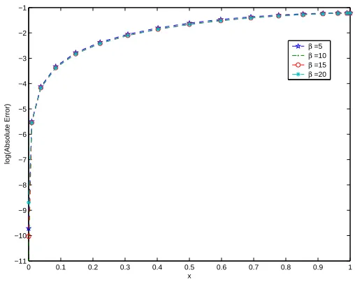
In Fig. 11, we plot log(absolute error) att= 1, N= 16, α= 2 and ∆t= 0.001 for Example 2.
0 0.1 0.2 0.3 0.4 0.5 0.6 0.7 0.8 0.9 1 −11
−10 −9 −8 −7 −6 −5 −4 −3 −2 −1
x
log(Absolute Error)
β =5
β =10
β =15
β =20
5. Conclusions
In this paper, a Chebyshev spectral collocation semi-discretization in space is applied to numerical solution of telegraph equation. We describe behavior of telegraph equation for various values of α and β at long time. Also we describe behavior of telegraph equation for various values ofN. The obtained results show that this approach can solve the problem effectively.
References
[1] M. Abdou, Adomian decomposition method for solving the telegraph equation in charged particle transport,J. Quant. Spectrosc. Radiat. Transfer, 95(2005) 407-414. [2] R. Baltensperger and M. R. Trummer, Spectral differencing with a twist,SIAM J. of
Sci. Comp., 24(5) (2003) 1465-1487.
[3] R. Baltensperger and J. P. Berrut, The errors in calculating the pseudospectral differ-entiation matrices for Chebyshev-Gauss-Lobatto point,Comput. Math. Appl., 37 (1999) 41-48.
[4] J. Biazar, M. Eslami, Analytic solution for Telegraph equation by differential transform method,Physics Letters A,374(29)(2010) 2904-2906.
[5] A. Borhanifar, R. Abazari, An unconditionally stable parallel difference scheme for telegraph equation scheme for telegraph equation,Math. Probl. Eng.(2009 (2009). [6] J. P. Boyd, Chebyshev and Fourier spectral methods, Lecture notes in engineering, 49,
Springer-verlag,Berlin(1989).
[7] C. Canuto, A. Quarteroni, M. Y. Hussaini and T. Zang, Spectral method in fluied mechanics,Springer-VerlagNew York (1988).
[8] W. S. Don and A. Solomonoff, Accuracy and speed in computing the Chebyshev collo-cation derivative,SIAM J. of Sci. Coput.,16(4)(1995) 1253-1268.
[9] S. Das, P. K. Gupta, Homotopy analysis method for solving fractional hyperbolic partial differential equations,International Journal of Computer Mathematics,88 (2011) 578-588.
[10] M. Dehghan, A. Ghesmati, Solution of the second-order one-dimensional hyperbolic telegraph equation by using the dual reciprocity boundary integral equation (DRBIE) method,Engineering Analysis with Boundary Elements,34 (2010) 51-59.
[11] M. Dehghan, A. Shokri, A numerical method for solving the hyperbolic telegraph equa-tion,Numer. Methods Partial Differential Equations,24 (2008) 1080-1093.
[12] M. Dehghan, M. Lakestani, The use of Chebyshev cardinal functions for solution of the second-order one-dimensional telegraph equation,Numer. Methods Partial Differential
Equations,25 (2009) 931-938.
[13] F. Gao, C. Chi, Unconditionally stable difference scheme for a one-space dimensional linear hyperbolic equation, Applied Mathematics and Computation, 187 (2007) 1272-1276.
[14] I. Hashim, O. Abdulaziz, S. Momani, Homotopy analysis method for fractional IVPs,
Communications in Nonlinear Science and Numerical Simulation,14 (2009) 674-684.
[15] M. Lakestani, B. N. Saray, Numerical solution of telegraph equation using interpolating scaling functions,Computers Mathematics with Applications,60 (2010) 1964-1972. [16] L. Lapidus, G. F. Pinder, Numerical Solution of Partial Differential Equations in Science
and Engineering,Wiley, New York, 1982.
[18] R. K. Mohanty, An unconditionally stable finite difference formula for a linear second order one space dimensional hyperbolic equation with variable coefficients,Appl. Math.
Comput., 165 (2005) 229-236.
[19] A. Mohebbi, M. Dehaghan, High order compact solution of the one dimensional linear hyperbolic equation,Numerical method for partial differential equations, 24 (2008) 1122-1135.
[20] A. Saadatmandi, M. Dehghan, Numerical solution of hyperbolic telegraph equation using the Chebyshev Tau method,Numer. Methods Partial Differential Equations,26(1) (2010) 239-252.
[21] L. N. Trefethen, Spectral methods in MATLAB, SIAM,Philadelphia(2000).