Max Planck Institute for Demographic Research Konrad-Zuse Str. 1, D-18057 Rostock·GERMANY www.demographic-research.org
DEMOGRAPHIC RESEARCH
VOLUME 27, ARTICLE 21, PAGES 593-644
PUBLISHED 9 NOVEMBER 2012
http://www.demographic-research.org/Volumes/Vol27/21/ DOI: 10.4054/DemRes.2012.27.21
Research Article
Point and interval forecasts of age-specific life
expectancies: A model averaging approach
Han Lin Shang
c
⃝2012 Han Lin Shang.
2 Revisiting the ten principal component approaches 595
2.1 Lee-Carter (LC) method 595
2.2 Lee-Miller (LM) method 596
2.3 Booth-Maindonald-Smith (BMS) method 597
2.4 Hyndman-Ullah (HU) method 597
2.5 Robust Hyndman-Ullah (HUrob) method 599 2.6 Weighted Hyndman-Ullah (HUw) method 599 2.7 Random walk with drift (RWD) method 600
2.8 Univariate time-series method 601
3 Model averaging approach 602
3.1 Literature review 602
3.2 Weight selection 604
3.2.1 A frequentist viewpoint 604
3.2.2 A Bayesian viewpoint 605
4 Data set 607
4.1 Training, validation, and forecasting data sets 608
5 Measures of point and interval forecast accuracy 609 5.1 Mean absolute forecast error and mean forecast error 609 5.2 Coverage probability deviance and half-width 609
6 Comparisons of the point forecasts 610
7 Comparisons of the interval forecasts 623
8 Result of the model averaging approach 633
9 Discussion 634
9.1 Point forecasts 635
9.2 Interval forecasts 635
9.3 Comparison with some previous findings 636
9.4 Limitations 636
9.5 Future research 637
9.6 Implementation 637
10 Acknowledgements 638
Point and interval forecasts of age-specific life expectancies:
A model averaging approach
Han Lin Shang1
Abstract
BACKGROUND
Any improvement in the forecast accuracy of life expectancy would be beneficial for policy decision regarding the allocation of current and future resources. In this paper, I revisit some methods for forecasting age-specific life expectancies.
OBJECTIVE
This paper proposes a model averaging approach to produce accurate point forecasts of age-specific life expectancies.
METHODS
Illustrated by data from fourteen developed countries, we compare point and interval fore-casts among ten principal component methods, two random walk methods, and two uni-variate time-series methods.
RESULTS
Based on averaged one-step-ahead and ten-step-ahead forecast errors, random walk with drift and Lee-Miller methods are the two most accurate methods for producing point fore-casts. By combining their forecasts, point forecast accuracy is improved. As measured by averaged coverage probability deviance, the Hyndman-Ullah methods generally provide more accurate interval forecasts than the Lee-Carter methods. However, the Hyndman-Ullah methods produce wider half-widths of prediction interval than the Lee-Carter meth-ods.
CONCLUSIONS
Model averaging approach should be considered to produce more accurate point forecasts.
COMMENTS
This study is a sequel to another Demographic Research paper by Shang, Booth and Hyndman (2011), in which the authors compared the principal component methods for forecasting age-specific mortality rates and life expectancy at birth.
1.
Introduction
In many developed countries, concerns of population aging are concentrated on the sus-tainability of pensions, health and age care systems. These concerns have resulted in a surge of interest among government policy makers and planners in accurately model-ing and forecastmodel-ing age-specific mortality rates and age-specific life expectancies. Any improvement in the forecast accuracy of life expectancy would be beneficial for policy decision regarding the allocation of current and future resources. In particular, future life expectancy is of great interest to the health care, age care, life insurance, superannua-tion and pensions industries. In these industries, the viability of financial arrangements depends on knowing the likelihood that clients will live to older ages.
In the demographic literature, a number of parametric and nonparametric methods have been put forward for forecasting age-specific mortality rates and life expectancy at birth (see for example, Preston, Heuveline, and Guillot 2001; Rowland 2003; Alho and Spencer 2005; Hyndman and Ullah 2007; Torri and Vaupel 2012). In a recent paper by Shang, Booth, and Hyndman (2011), they compared the point and interval forecast accuracy for forecasting age-specific mortality rates and life expectancy at birth, among ten principal component approaches. Differing from Shang, Booth, and Hyndman (2011), this paper serves two purposes. First, we compare the point and interval forecast accuracy of age-specific life expectancies, instead of the life expectancy at birth. We argue that the prediction of life expectancy at birth is of limited use in some situations. For instance, given a person aged 60, the pension industry would like to know his/her remaining life expectancy. Such information can be adequately supplied by forecasting age-specific life expectancies. Second, we put forward the idea of model averaging to improve point forecast accuracy. We hope that this paper will motivate the readers to consider the model averaging approach in the context of demographic forecasting.
and Ullah (2007) combined the ideas of nonparametric penalized regression spline and functional principal component analysis using second or higher order functional principal components.
In Section 3., we introduce a model averaging approach by combining forecasts from different models. We explore four ways of combining forecasts:
(1) assigning weights equally to all 14 models investigated in this paper;
(2) assigning weights to all 14 models based on their forecast accuracy in the validation data set;
(3) assigning weights to the best two models based on their forecast accuracy in the validation data set; and
(4) assigning weights using the notion of Bayesian model averaging (BMA), with Akaike’s (1974) weights.
Illustrated by the fourteen developed countries’ data sets described in Section 4., we cal-culate the point and interval forecasts of ten principal component methods, two naïve random walk methods, and two univariate time-series models for forecasting age-specific life expectancies. In Section 5., the criteria used to measure point and interval forecast accuracy are discussed. We evaluate and compare the point and interval forecast accu-racy among fourteen methods for forecasting age-specific life expectancies in Sections 6. and 7., respectively. In Section 8., we demonstrate the improvement of point forecast accuracy by combining forecasts with different weights. Conclusions are presented in Section 9., along with some thoughts on how the methods developed here might be fur-ther extended.
2.
Revisiting the ten principal component approaches
The next subsections specify the principal component models and notations, and describe the calculations of their point and interval forecasts of mortality rates. To start, letmx,t
be the log transformation of the mortality rate at agexin yeart. For forecasting mortal-ity rates, we are interested in obtaining estimates of age-specific mortalmortal-ity rates for one or more years of t > n(where nis the last observed year) as well as their associated measures of uncertainty.
2.1 Lee-Carter (LC) method
The LC model is given by
where
1. axis the age pattern of the log mortality rates averaged across years;
2. bx is the first principal component capturing relative change in the log mortality
rate at each agex, and∑px=0bx= 1;
3. ktis the first set of principal component scores measuring general level of the log
mortality rate at yeart;
4. ϵx,tis the model residual at agexand yeart, and
∑n
t=1kt= 0.
The LC model adjustsktby refitting to the total number of deaths. The adjustedktare
then extrapolated by a random walk with drift method, from which point forecasts are obtained by (1) with the fixedaxandbx.
Two sources of uncertainty should be considered: errors in the parameter estimation of the LC model and forecast errors in the forecast principal component scores. Because of the orthogonality2between the first principal component and the error term in (1), the
overall forecast variance can be approximated by the sum of the two variances. Condi-tioning on the past data pointsI and the first principal componentbx, we obtained the
overall forecast variance ofmx,n+h,
var[mx,n+h|I, bx]≈b2xun+h|n+vx, (2)
whereb2
x is the variance of the first principal component, calculated as the square of
the bx in (1); un+h|n = var(kn+h|k1, . . . , kn) can be obtained from the time-series
model; and the model residual variancevxis estimated by averaging the residual squares {ϵ2
x,1, . . . , ϵ2x,n}for eachxin (1).
There are two other methods that are closely related to the LC method. The first one is the LC method without adjustment ofkt, labeled as LCnone. The second one is the
Tuljapurkar, Li, and Boe’s (2000) method, labeled as TLB. The TLB method is the LC method without adjustment, and it also restricts the fitting period to 1950 onward.
2.2 Lee-Miller (LM) method
The LM method adjustsktso as to obtain the best forecasts of life expectancy at birth. It
differs from the LC method in three ways:
1. The jump-off rates are the actual rates in the jump-off year instead of the fitted rates for all other methods studied in this paper;
2. The fitting period begins in 1950;
3. The adjustment ofktinvolves fitting life expectancy at birth in yeart.
2.3 Booth-Maindonald-Smith (BMS) method
As a variant of the LC method, the BMS method differs from the LC method in three ways:
1. The fitting period is determined by a statistical “goodness of fit" criterion, under the assumption thatktis linear;
2. The adjustment ofktinvolves fitting to the age distribution of deaths rather than to
the total number of deaths;
3. The jump-off rates are the fitting rates under the fitting regime.
2.4 Hyndman-Ullah (HU) method
A possible weakness of the LC method and its variants is that they attempt to capture the patterns of age-specific mortality rates using only the first principal component and its associated scores. In addition, they do not implement a smoothing technique to smooth the mortality rates associated with old ages. To address this problem, Hyndman and Ullah (2007) proposed a functional data model that utilizes second and higher order ones to capture additional variation in mortality rates.
The method proposed by Hyndman and Ullah (2007) combines the nonparametric pe-nalized regression spline of Ramsay (1988) with functional principal component analysis of Ramsay and Dalzell (1991) for forecasting mortality rates. The HU method differs from the LC method in three ways:
1. The log mortality rates are first smoothed using a penalized regression spline with a partial monotonic constraint (see Ramsay 1988, for detail). We assume that there is an underlying continuous and smooth functionft(x)that is observed with errors
at discrete ages. Expressed mathematically,
mt(xi) =ft(xi) +σt(xi)ϵt,i, i= 1, . . . , p, t= 1, . . . , n, (3)
wheremt(xi)represents the log transformation of the observed mortality rate for
agexiin yeart,σt(xi)allows the noise component to vary withxiin yeart, and
ϵt,iis independent and identically distributed standard random variable.
2. More than one principal component is used. By functional principal component analysis, a set of continuous functions is decomposed into functional principal com-ponents and their associated scores. That is,
ft(x) =a(x) +
J
∑
j=1
where
(1) a(x)is the mean function estimated by empirical meanba(x) =n1∑nt=1ft(x);
(2) {b1(x), . . . , bJ(x)}represents a set of the firstJ functional principal
compo-nents;
(3) {kt,1, . . . , kt,J}represents a set of uncorrelated principal component scores;
(4) et(x)is the residual function with mean zero and variancev(x)estimated by
averaging{e21(x), . . . , e2n(x)};
(5) J < nis the optimal number of functional principal components used.
Fol-lowing Hyndman and Booth (2008) and Shang, Booth, and Hyndman (2011), we choseJ = 6which should be larger than any of the components required. 3. A broader range of univariate time-series models may be used to forecast the princi-pal component scores. By conditioning on the past smooth curves I =
{m1(x), . . . , mn(x)} and the set of functional principal components B =
{b1(x), . . . , bJ(x)}, theh-step-ahead point forecast ofmn+h(x)can be obtained
by
b
mn+h|n(x) =E[mn+h(x)|I,B] =ba(x) +
J
∑
j=1
bj(x)bkn+h|n,j,
wherebkn+h|n,jdenotes theh-step-ahead forecast ofkn+h,jusing a univariate
time-series model, such as the ARIMA model (Box, Jenkins, and Reinsel 2008) used in this paper. The optimal order of an ARIMA model is automatically selected using an algorithm of Hyndman and Khandakar (2008), which minimizes the Akaike information criterion (Akaike 1974) by default.
The forecast variance follows from (3) and (4). Due to the orthogonality3 between the functional principal components and the error term, the overall forecast variance can be approximated by the sum of four individual variances. Conditioning on the past smooth curvesIand the set of fixed principal componentsB={b1(x), . . . , bJ(x)}, we obtained
the overall forecast variance ofmn+h(x),
var[mn+h(x)|I,B]≈bσa2(x) + J
∑
j=1
b2j(x)un+h|n,j+v(x) +σn2+h(x), (5)
where
(1) σb2
a(x)is the variance of the smooth estimate ba(x)that can be obtained from the
smoothing method. (2) b2
j(x)is the variance of thejth principal component;
un+h|n,j=var(kn+h,j|k1,j, . . . , kn,j)can be obtained from the time-series model.
(3) the model residual variancev(x)is estimated by averaging{e2
1(x), . . . , e2n(x)}for
eachx;
(4) the observational error varianceσn2+h(x)is estimated by averaging{bσ12(x), . . . ,bσn2(x)}
for eachx(Hyndman and Ullah 2007).
By assuming that each of the four sources of uncertainty have a normal distribution and that they are uncorrelated, the100(1−α)%prediction interval ofmn+h(x)is constructed
as mbn+h|n(x)±zα
√
var[mn+h(x)|I,B], where zα is the(1−α/2)standard normal
quantile.
2.5 Robust Hyndman-Ullah (HUrob) method
Because the presence of outliers can seriously affect the performance of modeling and forecasting, it is important to eliminate the effect of outliers where possible. The HUrob method calculates the integrated squared error for each year,
∫ xp
x1
(
ft(x)−a(x)−
J
∑
j=1
bj(x)kt,j
)2
dx,
as this provides a measure of estimation accuracy for the functional principal compo-nent approximation of the functional data. Note that the continuous functional curves are bounded betweenx1andxp. Outliers are those years that have a larger integrated squared
error than the critical value calculated from a χ2 distribution (see Hyndman and Ullah 2007, for detail). By assigning zero weight to outliers, we can apply the HU method to model and forecast mortality rates, from which forecasts of age-specific life expectancies are calculated without influence of possible outliers.
2.6 Weighted Hyndman-Ullah (HUw) method
The HUw method uses geometrically decaying weights in the estimation ofa(x) and
bj(x), thus allowing the estimation of these quantities to be based more on recent data than
on data from the distant past (Hyndman and Shang 2009; Shang, Booth, and Hyndman 2011).
1. The weighted functional meana∗(x)is estimated by
b
a∗(x) =
n
∑
t=1
wtft(x),
n
∑
t=1
wt= 1,
where{wt=κ(1−κ)n−t, t= 1, . . . , n}denotes a set of weights, and0< κ <1
denotes a geometrically decaying weight parameter. Hyndman and Shang (2009) describe how to estimate the optimal value ofκempirically from data. In short, the optimal value ofκ∈ (0,1)is chosen by minimizing an overall forecast error measure within the validation data set among a set of possible candidates. In this paper, we utilize a one-dimensional optimization algorithm of Nelder and Mead (1965) to minimize the objective function and to find its corresponding optimal (exact) value ofκ.
2. By functional principal component analysis, a set of weighted functions{wt[ft(x)−
b
a∗(x)];t = 1, . . . , n} is decomposed into weighted functional principal
compo-nents and their uncorrelated principal component scores. That is,
ft(x) =ba∗(x) +
J
∑
j=1
b∗j(x)kt,j+et(x),
where{b∗1(x), . . . , b∗J(x)}is a set of weighted functional principal components. 3. Conditioning on the past smooth curvesI ={m1(x), . . . , mn(x)}and the set of
weighted functional principal componentsB∗ = {b∗1(x), . . . , b∗J(x)}, theh
-step-ahead forecast ofmn+h(x)is obtained by
b
mn+h|n(x) =E[mn+h(x)|I,B] =ba∗(x) +
J
∑
j=1
b∗j(x)kn+h|n,j.
From the variance expression given by (5), the100(1−α)%prediction interval of future mortality rates at yearn+his constructed parametrically.
2.7 Random walk with drift (RWD) method
While Sections 2.1-2.6 introduce various principal component methods to forecast age-specific mortality rates and calculate survival probabilities, from which we can derive remaining life expectancy by age. In this subsection, we revisit two naïve random walk methods that are able to forecast the life expectancy for each age.
point forecast accuracy of the principal component methods with linear extrapolation of life expectancy (see Alho and Spencer 2005, pp.274-276 for an introduction). The linear extrapolation of age-specific life expectancies was achieved by applying the random walk with drift (RWD) model for each age:
yx,t+1=d+yx,t+ex,t+1, t= 1,2, . . . , n−1, x= 0,1, . . . , p. (6)
whereyx,trepresents the life expectancy at agexin yeart. Theh-step-ahead point and
interval forecasts are given by
b
yx,n+h|n=E[yx,n+h|yx,1, . . . , yx,n] =dh+yx,n,
var(ybx,n+h|n) =var[yx,n+h|yx,1, . . . , yxn] =var(yx,n) +var(ex,n+h). (7)
Based on (6) to (7), the random walk without drift, labeled as RW, can be obtained simply by omitting the drift term. Computationally, the forecasts of RW and RWD methods are obtained by the rwffunction in the forecastpackage (Hyndman 2012b) in R (R Development Core Team 2012).
2.8 Univariate time-series method
One popular approach to forecasting age-specific life expectancies involves the use of univariate time-series models. In this approach, we select a particular time-series model for the series to be forecasted, and use the fitted model to produce point and interval forecasts for each age. The ARIMA model discussed by Box, Jenkins, and Reinsel (2008) comprises one popular class of models (see also its equivalent exponential smoothing (ETS) state-space model of Hyndman, Koehler, Ord, and Snyder 2008). The ARIMA model has been applied to forecast life expectancy and its related problems by Torri and Vaupel (2012) for example.
The ARIMA model is designed to handle stationary and non-stationary stochastic processes. In general notation, we have an ARIMA(p, d, q) model, wherepis the order of the autoregressive component,dindicates the order of integration, that is, how many times the series must be differenced in order to achieve the stationarity, andqis the order of the moving average component. For simplicity, we consider a stationary time series. The ARMA(p, q) model for a univariate time series(yx,1, yx,2, . . . , yx,n)is given by
yx,t−µ=
p
∑
i=1
ϕi(yx,t−i−µ)
| {z }
AR(p)
+ϵx,t+
q
∑
j=1
θjϵx,t−j
| {z }
MA(q)
where the constant parameterµis the drift term, representing the average change in the se-ries over time;ϕiare the parameters of the autoregressive component, and likewiseθjare
the parameters of the moving average component, andϵx,tis a sequence of independent
and identically distributed random variables with mean zero and varianceσ2
w.
Following the early work by Box, Jenkins, and Reinsel (2008, p.218), the one-step-ahead point forecasts and overall variance are given by
b
yx,n+1|n=E[yx,n+1|yx,1, yx,2, . . . , yx,n] =µb+
p
∑
i=1
b
ϕi(yx,n+1−i−µb), (8)
var[yx,n+1|yx,1, yx,2, . . . , yx,n] =bσw2
(
1 +θb12+bθ22+· · ·+θb2q
)
, (9)
from the overall variance, a100(1−α)%prediction interval ofyx,n+1can be constructed parametrically for each age. The parameters are commonly estimated by the maximum likelihood criterion. For theh-step-ahead forecasts, (8) and (9) can be applied iteratively. A difficulty associated with the use of ARIMA model is the order selection. Hynd-man and Khandakar (2008) developed an algorithm, namedauto.arimain theforecast package in R, for automatically selecting the optimal orders based on a statistical criterion, such as Akaike’s (1974) information criterion.
3.
Model averaging approach
3.1 Literature review
Suppose a decision maker is forecasting the values of some variables, such asmn+h|n(x).
He is given L different forecasts of the values mbn+h|n(x), namely mb
(1)
n+h|n(x), . . . ,
b
m(nL+)h|n(x). Because theseLdifferent forecasts may reflect different assumptions, model structures and degree of model complexity, he does not want to simply choose the best one and discard the rest. Instead, he would like to combine these forecasts to get a better forecast accuracy.
opti-mal weights to attach to these two original forecasts in forming the combined forecasts4.
The review paper by Clemen (1989) collected a number of contributions on the idea of combining forecasts in the fields of forecasting, psychology, statistics, and management science. While Bates and Granger (1969) and Dickinson (1975) discussed a way of se-lecting optimal weights from a frequentist viewpoint, Bunn (1975) and Bordley (1982) provided an alternative Bayesian derivation of optimal weights, and showed the similarity with the frequentist viewpoint. An excellent review article on BMA is given by Hoeting et al. (1999).
By using the model averaging approach, one can obtain a better accuracy than any method alone, when the forecasts combined use different methods that capture different information, different specifications or different assumptions. Because the underlying data generating process is often unknown, combined forecasts are more robust toward model mis-specification and are more likely to produce accurate point forecasts. In the demographic literature, there has been little interest in combining forecasts from different models. Nonetheless, some notable exceptions include Smith and Shahidullah (1995); Ahlburg (1998, 2001) and Sanderson (1998), whose pioneering work, particularly in the context of census tract forecast, have done much to awaken others, including the present author. The contribution of this article is to apply the notion of model averaging to the problem of forecasting age-specific life expectancies.
In the work by Smith and Shahidullah (1995), it was found that a forecast of cen-sus tract population based on simple average of forecasts from four extrapolation tech-niques5 was as accurate as the single most accurate method. By combining forecasts
from two methods that were found to predict accurately for particular types of tracts, they asserted that using knowledge of historical forecast performance can further reduce fore-cast error when combined. Ahlburg (1998) also demonstrated that combined forefore-casts of births from an economic demographic model and from the U.S. Bureau of census’ cohort-component model produced more accurate forecast than the official cohort-cohort-component forecasts alone, indeed with a 15% decrease in the mean absolute percentage error. Fur-thermore, Sanderson (1998) stated that combining casual economic-demographic models for developing countries produced better forecasts than demographic cohort-component forecasts. With a 21% reduction in the mean absolute percentage error, the combined forecasts produced better results than does reliance on only one forecast method.
4See also Section 3.2.1.
3.2 Weight selection
3.2.1 A frequentist viewpoint
There are two common questions raised from the model averaging approach, which may be of interest to demographers and statisticians. The first one is: how many models should be included in the combination? From the frequentist viewpoint, Schmittlein, Kim, and Morrison (1990) used the Akaike’s (1974) information criterion to decide. From the Bayesian viewpoint, Madigan and Raftery (1994) suggested that if a model predicts the data far less well than the model which provides the best predictions, then it should be omitted from model combination. In what follows, we consider two situations, namely combining two best approaches and combining all approaches. The optimal weights are selected by their past forecast errors in the validation data set.
Two best models: Following the work of Bates and Granger (1969), our initial model averaging approach combines forecasts from two models given as follows:
b
yn+h|n,combo =λybn+h|n,M1+ (1−λ)ybn+h|n,M2,
whereybn+h|n,M1 andybn+h|n,M2represent the point forecasts obtained from two models,
labeled asM1andM2respectively;ybn+h|n,comborepresents the combined forecasts; and
0< λ <1is the weight parameter that needs to be estimated in light of data. Asλ→0,
b
yn+h|n,combo→ybn+h|n,M2, asλ→1,ybn+h|n,combo→ybn+h|n,M1.
Libby and Blashfield (1978) reported that the majority of the improvement in accuracy was achieved with the combination of the top two forecasts. By combining forecasts from two methods, we have only one parameterλto be determined from data, and this simplifies the optimization procedure in determining the value ofλ.
Between the two best approaches, we calculate the point forecast accuracy as mea-sured by the MAFEs in the validation set, and assign the weights to be the inverse of their MAFEs (that isMAFE1 ). To avoid the possible model identification, the sum of the weights must be equal to 1, therefore, we normalize the weights
(
each weight sum of weights
)
.
Conceptually, the method that performs better in the validation set receives a higher weight in the combined forecasts. Note that one can also iteratively update the optimal weights successively by taking into account the most recent data. Here, we implicitly assume that future age-specific life expectancies do not change significantly over years, which is a reasonable assumption (see also White 2002; Oeppen and Vaupel 2002).
model averaging approach combines forecasts from 14 models given as follows:
b
yn+h|n,combo =
η1ybn+h|n,M1+η2byn+h|n,M2+η3ybn+h|n,M3+η4ybn+h|n,M4+η5ybn+h|n,M5
+η6ybn+h|n,M6+η7ybn+h|n,M7+η8byn+h|n,M8+η9byn+h|n,M9+η10ybn+h|n,M10
+η11ybn+h|n,M11+η12ybn+h|n,M12+η13byn+h|n,M13+ (1−η1−η2−η3−η4
−η5−η6−η7−η8−η9−η10−η11−η12−η13)ybn+h|n,M14,
whereybn+h|n,M1,ybn+h|n,M2, . . . ,ybn+h|n,M14represent the point forecasts obtained from
the 14 models, labeled asM1, M2, . . . , M14respectively, (η1, η2, . . . , η13)represents a set of weights.
For all approaches, we calculate the point forecast accuracy as measured by the MAFEs in the validation set, and assign the weights to be the inverse of their MAFEs (that is
1
MAFE). To avoid the possible model identification, the sum of the weights must be equal
to 1, therefore, we normalize the weights
(
each weight sum of weights
)
.
3.2.2 A Bayesian viewpoint
The second question is: what is the best way of selecting optimal weights? While Sec-tion 3.2.1 presents a frequentist way of selecting optimal weights, in this subsecSec-tion we discuss a Bayesian means of determining optimal weights. From the Bayesian viewpoint, BMA is another solution to the model uncertainty problem (see, for example, Wright 2008; Geweke and Amisano 2012). LetM1, M2, . . . , MK be a set ofKpossible models
and one of the models is the true model. Letθ1, θ2, . . . , θK be the vector of parameters
associated with each model. Denote∆ as the quantity of interest, such as a combined forecast of age-specific life expectancies, then its posterior distribution given dataDis
P r(∆|D) =
K
∑
k=1
P r(∆|Mk, D)P r(Mk|D),
=
K
∑
k=1
P r(∆|Mk, D)
P r(D|Mk)
∑K
l=1P r(D|Ml)P r(Ml)
| {z }
weights
, (10)
where Pr(D|Mk) =
∫
Pr(D|θk, Mk)Pr(θk|Mk)dθk. Pr(θk|Mk)is the prior density ofθk
under modelMk, Pr(D|θk, Mk)is the likelihood, Pr(Mk)is the prior probability thatMk
of the models considered, weighted by their posterior model probability (Hoeting et al. 1999).
Given diffuse priors and equal model prior probabilities, the BMA weights are approx-imately
wk=
exp(−1
2BICk
)
∑K
k=1exp
(
−1 2BICk
),
where
BICk = 2Lk+ log(n)λk,
whereLkis the negative log-likelihood,λkis the number of parameters in modelk, BICk
is the Bayesian information criterion for modelk(see also Burnham and Anderson 2004). The BMA estimator has a nice interpretation from a Bayesian viewpoint. The down-side is that the “true" model must be in the set ofKpossible models. To remedy this situation, Burnham and Anderson (2002) suggested replacing BIC with AIC, and we fol-low this idea in this paper. The weights are given by
wk =
exp(−12AICk)
∑K
k=1exp(− 1 2AICk)
, (11)
where
AICk = 2Lk+ 2λk,
=nlog
(
RSSk
n
)
+ 2λk,
wherenis the sample size, and RSS is the residual sum of squares for each model (Burn-ham and Anderson 2004).
The individual AIC values are not interpretable, as they contain arbitrary constants and are much affected by sample size. Here, it is imperative to rescale AIC to
AICdiff,k=AICk−AICmin, (12)
where AICminis the minimum of theKdifferent AICk values. Plugging (12) into (11),
4.
Data set
The data sets used in this study were taken from the Human Mortality Database (2012). Note that in the Human Mortality Database (2012), a full-fledged life table is calculated systematically and age-specific life expectancies are presented in the last column for each gender and country. Fourteen developed countries were selected, and thus 28 sex-specific populations were obtained for all analyses. The selected fourteen countries all have reli-able data series commencing before 1950, which is the starting year of the fitting period for the LM method. The selected countries are presented in Table 1, along with their initial fitting period.
Table 1: Commencing years of the initial fitting period for different methods and countries
Country LC LCnone TLB LM BMS[f] BMS[m] RWD RW
Australia 1921 1921 1950 1950 1962 1958 1921 1921
Canada 1921 1921 1950 1950 1954 1954 1921 1921
Denmark 1835 1835 1950 1950 1948 1948 1835 1835
England 1841 1841 1950 1950 1952 1953 1841 1841
Finland 1878 1878 1950 1950 1962 1956 1878 1878
France 1816 1816 1950 1950 1946 1946 1816 1816
Iceland 1838 1838 1950 1950 1946 1947 1838 1838
Italy 1872 1872 1950 1950 1962 1958 1872 1872
Netherlands 1850 1850 1950 1950 1947 1947 1850 1850
Norway 1846 1846 1950 1950 1948 1948 1846 1846
Scotland 1855 1855 1950 1950 1960 1970 1855 1855
Spain 1908 1908 1950 1950 1952 1953 1908 1908
Sweden 1751 1751 1950 1950 1932 1953 1751 1751
Table 1: (Continued)
Country HU HU50 HUrob HUrob50 HUw ETS ARIMA
Australia 1921 1950 1921 1950 1921 1921 1921
Canada 1921 1950 1921 1950 1921 1921 1921
Denmark 1835 1950 1835 1950 1835 1835 1835
England 1841 1950 1841 1950 1841 1841 1841
Finland 1878 1950 1878 1950 1878 1878 1878
France 1816 1950 1816 1950 1816 1816 1816
Iceland 1838 1950 1838 1950 1838 1838 1838
Italy 1872 1950 1872 1950 1872 1872 1872
Netherlands 1850 1950 1850 1950 1850 1850 1850
Norway 1846 1950 1846 1950 1846 1846 1846
Scotland 1855 1950 1855 1950 1855 1855 1855
Spain 1908 1950 1908 1950 1908 1908 1908
Sweden 1751 1950 1751 1950 1751 1751 1751
Switzerland 1876 1950 1876 1950 1876 1876 1876
Notes: Although the RW model depends only on the previous year, the variance of the RW model requires all data.
4.1 Training, validation, and forecasting data sets
We divide each data set into a fitting period(1 :n−20)and a forecasting period(n−19 : n), wherendenotes the last year of observations in a data set. The commencing year of the fitting period differs by method, as seen in Table 1. We implement a rolling origin regime as follows: the forecasting period is set to be the last 20 years, all ending in 2007, while the remaining data are in the initial fitting period. Using the data in the fitting period, we compute the one-step-ahead and ten-step-ahead point and interval forecasts, and determine the forecast accuracy by comparing the forecasts with the holdout data in the forecasting period. Then, we increase the fitting period by one year, and compute the one-step-ahead and ten-step-ahead point and interval forecasts, and calculate the point and interval forecast accuracy. This process is repeated until the forecasts reach the last year of available data.
Within the fitting period, we further split the data into a training period(1 :n−40)
5.
Measures of point and interval forecast accuracy
There exist a number of criteria for measuring point and interval forecast accuracy. In Sections 5.1 and 5.2, we present two criteria each for measuring the point and interval forecast accuracy.
5.1 Mean absolute forecast error and mean forecast error
By using thedemographicpackage (Hyndman 2012a) in R, we calculate the point and interval forecasts for each method, and evaluate and compare their forecast accuracy. To measure point forecast accuracy and bias, we utilize the mean absolute forecast error and mean forecast error, labeled as MAFE and MFE. These two criteria have previously been implemented in Shang, Booth, and Hyndman (2011) and Booth et al. (2006), although one can also use mean absolute percentage forecast error and mean algebraic percentage fore-cast error to measure the accuracy and bias, respectively. The MAFE criterion measures how close the forecasts come to the actual values of the variable being forecast, regardless of the sign of error. In contrast, the MFE is the average of errors, (actual - forecast), and is a measure of bias. These measures can be expressed mathematically as
MAFE= 1
(p+ 1)×q
q
∑
j=1
p
∑
x=0
yx,j−ybx,j|j−h, j= (n−20 +h), . . . , n
MFE= 1
(p+ 1)×q
q
∑
j=1
p
∑
x=0
(
yx,j−ybx,j|j−h
)
,
whereqrepresents the number of years in the forecasting period,yx,jrepresents the actual
holdout sample for agexin yearj, andbyx,jrepresents the forecasts for the holdout sample.
We consider the one-step-ahead and ten-step-ahead forecasts in this paper.
5.2 Coverage probability deviance and half-width
calculated the coverage probability deviance, which is the absolute difference between the nominal coverage probability and the empirical coverage probability. With the nominal coverage probability of 0.8, the maximum coverage probability deviance is 0.8 when the empirical coverage probability is 0; while the minimum coverage probability deviance is 0 when the empirical coverage probability is 0.8.
Apart from the coverage probability deviance, we also calculate the size of the pre-diction interval. Following the early work by Lee and Tuljapurkar (1994) and Tayman, Smith, and Lin (2007), the size of the prediction interval is defined as half-width by divid-ing one-half of the difference between the upper and lower bounds of the interval forecasts. For the symmetric interval, the half-width reflects the distance between the point forecast (center) and the lower and upper bounds of the prediction interval.
6.
Comparisons of the point forecasts
For simplicity, we will refer to the LC method and its variants6as the LC methods, and refer to the HU method and its variants7 as the HU methods. Results are presented by
country and for two averages: the simple average and a weighted average using weights based on population size in 2007. For each country, the weight is calculated as the coun-try’s population size in 2007 divided by the sum of each councoun-try’s population size and scaled to sum to 14. For females, the weights are 0.87, 1.36, 0.23, 2.55, 0.21, 2.63, 0.01, 2.50, 0.68, 0.19, 0.22, 1.86, 0.38, 0.32 in the country order of Table 1. For males, the weights are 0.89, 1.39, 0.23, 2.55, 0.23, 2.56, 0.01, 2.46, 0.69, 0.20, 0.21, 1.88, 0.39, 0.31. Hereafter, the simple average is labeled by Mean, while the weighted average is labeled by Mean(w).
6all based on a single principal component
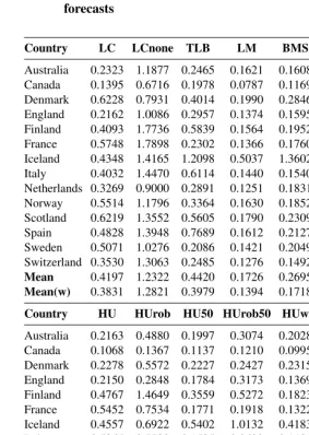
Table 2: Point forecast accuracy of the female life expectancies by method and country, as measured by the MAFEs for the one-step-ahead forecasts
Country LC LCnone TLB LM BMS RWD RW
Australia 0.2323 1.1877 0.2465 0.1621 0.1608 0.1586 0.1904
Canada 0.1395 0.6716 0.1978 0.0787 0.1169 0.0782 0.1155
Denmark 0.6228 0.7931 0.4014 0.1990 0.2846 0.1838 0.1886
England 0.2162 1.0086 0.2957 0.1374 0.1595 0.1370 0.1659
Finland 0.4093 1.7736 0.5839 0.1564 0.1952 0.1480 0.1741
France 0.5748 1.7898 0.2302 0.1366 0.1760 0.1357 0.1696
Iceland 0.4348 1.4165 1.2098 0.5037 1.3602 0.3804 0.3885
Italy 0.4032 1.4470 0.6114 0.1440 0.1540 0.1442 0.1855
Netherlands 0.3269 0.9000 0.2891 0.1251 0.1831 0.1184 0.1351
Norway 0.5514 1.1796 0.3364 0.1630 0.1852 0.1533 0.1666
Scotland 0.6219 1.3552 0.5605 0.1790 0.2309 0.1738 0.1986
Spain 0.4828 1.3948 0.7689 0.1612 0.2127 0.1534 0.1621
Sweden 0.5071 1.0276 0.2086 0.1421 0.2049 0.1309 0.1440
Switzerland 0.3530 1.3063 0.2485 0.1276 0.1492 0.1158 0.1496
Mean 0.4197 1.2322 0.4420 0.1726 0.2695 0.1580 0.1810
Mean(w) 0.3831 1.2821 0.3979 0.1394 0.1718 0.1363 0.1651
Country HU HUrob HU50 HUrob50 HUw ETS ARIMA
Australia 0.2163 0.4880 0.1997 0.3074 0.2028 0.1449 0.1493
Canada 0.1068 0.1367 0.1137 0.1210 0.0995 0.0987 0.0896
Denmark 0.2278 0.5572 0.2227 0.2427 0.2315 0.2184 0.1967
England 0.2150 0.2848 0.1784 0.3173 0.1369 0.1433 0.1412
Finland 0.4767 1.4649 0.3559 0.5272 0.1823 0.1430 0.1610
France 0.5452 0.7534 0.1771 0.1918 0.1322 0.1478 0.1707
Iceland 0.4557 0.6922 0.5402 1.0132 0.4183 0.3415 0.3400
Italy 0.5265 0.7780 0.1535 0.2693 0.1486 0.1504 0.1899
Netherlands 0.1798 0.3873 0.2618 0.2085 0.1417 0.1466 0.1938
Norway 0.6440 0.6547 0.2870 0.4187 0.1955 0.1493 0.1614
Scotland 0.4560 1.0595 0.4033 0.3977 0.3137 0.1601 0.1906
Spain 0.2578 0.2695 0.1550 0.4092 0.1633 0.1439 0.1502
Sweden 0.4139 1.8243 0.1550 0.1816 0.1501 0.1688 0.1260
Switzerland 0.3233 0.6789 0.1480 0.2939 0.3370 0.1279 0.1319
Mean 0.3603 0.7164 0.2394 0.3500 0.2038 0.1632 0.1709
Table 3: Point forecast accuracy of the male life expectancies by method and country, as measured by the MAFEs for the one-step-ahead forecasts
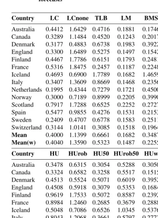
Country LC LCnone TLB LM BMS RWD RW
Australia 0.4412 1.6429 0.4716 0.1881 0.1746 0.1798 0.2254 Canada 0.3289 1.1484 0.4520 0.1243 0.2017 0.1219 0.1672 Denmark 0.3177 0.4883 0.6738 0.1983 0.3922 0.1613 0.1787 England 0.3300 1.6489 0.5275 0.1497 0.1542 0.1377 0.1995 Finland 0.4467 1.7786 0.6151 0.1793 0.2481 0.1520 0.1924 France 0.5316 1.8475 0.2457 0.1187 0.2248 0.1340 0.1724 Iceland 0.4693 0.6900 1.7789 0.1682 1.4659 0.4099 0.4173 Italy 0.3407 1.3609 0.8669 0.1468 0.2356 0.1331 0.1876 Netherlands 0.1995 0.4344 0.7279 0.1721 0.4500 0.1463 0.1814 Norway 0.3000 0.7189 0.8999 0.2205 0.3990 0.1887 0.2179 Scotland 0.7917 1.7288 0.6525 0.2252 0.2727 0.1890 0.2094 Spain 0.5477 0.9855 0.4276 0.1531 0.2153 0.1467 0.1502 Sweden 0.2409 0.4707 0.6778 0.1583 0.2511 0.1381 0.1681 Switzerland 0.3144 1.0141 0.3085 0.1518 0.1964 0.1361 0.1930
Mean 0.4000 1.1399 0.6661 0.1682 0.3487 0.1696 0.2043
Mean(w) 0.4040 1.3590 0.5323 0.1487 0.2255 0.1412 0.1825
Country HU HUrob HU50 HUrob50 HUw ETS ARIMA
Australia 0.3478 0.6315 0.3054 0.5288 0.3050 0.1508 0.1636 Canada 0.3324 0.6582 0.3258 0.5517 0.1515 0.1080 0.1086 Denmark 0.4513 0.5524 0.5071 0.6019 0.3952 0.2331 0.2374 England 0.4508 0.5918 0.3079 0.5353 0.1684 0.1631 0.1966 Finland 0.9619 1.7533 0.5072 0.8587 0.2392 0.2875 0.3284 France 0.8984 1.2460 0.2685 0.3679 0.2888 0.1340 0.3174 Iceland 0.5048 0.7086 0.6526 1.0345 0.5376 0.5313 0.4443 Italy 0.8043 1.2068 0.3661 0.5797 0.2772 0.2130 0.3343 Netherlands 0.4320 0.3337 0.5156 0.5521 0.1786 0.2676 0.2197 Norway 0.4169 0.4796 0.3140 0.8530 0.4196 0.2510 0.2331 Scotland 0.7227 0.9819 0.6266 0.7011 0.5822 0.2187 0.2357 Spain 0.3512 0.3285 0.3165 0.3493 0.1636 0.1628 0.1437 Sweden 0.5420 0.7789 0.4691 0.6572 0.3945 0.2350 0.3957 Switzerland 0.6003 1.1496 0.3517 0.3479 0.4686 0.2210 0.2416
Mean 0.5583 0.8143 0.4167 0.6085 0.3264 0.2269 0.2571
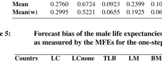
Tables 2 and 3 provide summaries of the point forecast accuracy based on the MAFEs for the one-step-ahead forecasts of life expectancies. The summaries given in Tables 2 and 3 are averaged over different ages from 0 to 104, and years in the forecasting period for female and male data, respectively. As measured by the simple and weighted averages of MAFEs over the fourteen countries, the RWD method produces the most accurate point forecasts in both female and male data. The performance of RWD method is followed closely by the LM method.
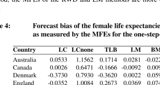
Tables 4 and 5 show the corresponding MFEs for the one-step-ahead point forecasts. For the female data, the LCnone, HU, HUrob and RW methods consistently underesti-mate8 the life expectancies for all countries, while the other methods exhibit a mixture of overestimation and underestimation for various countries. Of all the methods, the LM method performs the best as measured by both the simple and weighted averages. The performance of the LM method is followed by the BMS and RWD methods. For the male data, all methods consistently underestimate the life expectancies except the LC method. Cancelation of MFEs from different countries leads to the most superior performance of the LC method, which is followed by the RWD and LM methods. In contrast to the LC method, the MFEs of the RWD and LM methods are more centered around zero at all ages.
Table 4: Forecast bias of the female life expectancies by method and country, as measured by the MFEs for the one-step-ahead forecasts
Country LC LCnone TLB LM BMS RWD RW
Australia 0.0533 1.1562 0.1714 0.0281 -0.0226 0.0460 0.1399
Canada 0.0026 0.6471 -0.1666 -0.0092 0.0090 -0.0129 0.0922
Denmark -0.3730 0.7930 -0.3620 0.0022 0.0599 0.0126 0.0749
England -0.0352 1.0084 0.2673 0.0369 0.0741 0.0169 0.1196
Finland -0.1378 1.7457 0.4936 -0.0001 -0.0453 0.0472 0.1426
France -0.2436 1.7898 0.1183 -0.0089 0.0154 0.0643 0.1384
Iceland 0.2496 1.3925 1.1813 0.2797 1.3262 0.0000 0.0876
Italy -0.1577 1.4352 0.6083 0.0167 0.0135 0.0297 0.1439
Netherlands -0.1329 0.8848 -0.2780 -0.0271 -0.0374 -0.0143 0.0657
Norway -0.3223 1.1683 0.2193 0.0107 -0.0080 0.0402 0.1020
Scotland -0.2684 1.3552 0.4348 0.0196 0.0852 0.0383 0.1063
Spain -0.2360 1.3167 0.7206 -0.0208 0.1102 -0.0145 0.1204
Table 4: (Continued)
Country LC LCnone TLB LM BMS RWD RW
Sweden -0.3017 1.0144 -0.1267 -0.0064 -0.0254 0.0363 0.0870
Switzerland -0.1650 1.2868 -0.0239 -0.0323 -0.0490 -0.0032 0.1129
Mean -0.1477 1.2139 0.2327 0.0204 0.1076 0.0205 0.1095
Mean(w) -0.1431 1.2631 0.2644 0.0046 0.0318 0.0224 0.1217
Australia 0.1467 0.4563 0.1393 0.2633 0.0128 0.0493 0.0660
Canada 0.0080 0.0760 -0.0091 -0.0233 -0.0013 -0.0159 -0.0154
Denmark 0.0667 0.5339 -0.0777 -0.0753 0.1722 0.0062 0.0196
England 0.1632 0.2577 0.1189 0.2742 0.0784 0.0788 0.0814
Finland 0.4319 1.4370 0.2610 0.4631 0.0332 0.0641 0.0837
France 0.5290 0.7473 0.0801 0.1528 0.0041 0.0643 0.1173
Iceland 0.0068 0.5514 0.4013 0.9595 0.2352 0.0619 0.0176
Italy 0.5189 0.7585 0.0619 0.2261 0.0867 0.0722 0.0944
Netherlands 0.0622 0.3352 -0.1936 -0.1417 0.0538 -0.0331 -0.1026
Norway 0.6257 0.5736 0.1882 0.3672 0.1287 0.0723 0.0791
Scotland 0.4352 1.0481 0.3214 0.2523 0.2674 0.0489 0.1110
Spain 0.1855 0.2229 0.0831 0.3268 0.0639 -0.0350 -0.0364
Sweden 0.3888 1.7578 -0.0842 0.0701 0.0834 0.1450 0.0456
Switzerland 0.2955 0.6572 0.0020 0.2429 0.3133 -0.0698 -0.0358
Mean 0.2760 0.6724 0.0923 0.2399 0.1094 0.0364 0.0375
Mean(w) 0.2995 0.5221 0.0655 0.1925 0.0612 0.0398 0.0513
Table 5: Forecast bias of the male life expectancies by method and country, as measured by the MFEs for the one-step-ahead forecasts
Country LC LCnone TLB LM BMS RWD RW
Australia 0.0873 1.5445 0.4189 0.0956 0.0633 0.1212 0.1953
Canada 0.1906 1.0953 0.4129 0.0903 0.1656 0.0899 0.1501
Denmark -0.0175 0.1804 0.6120 0.1042 0.3456 0.0679 0.1203
England 0.1309 1.6489 0.5142 0.1093 0.1054 0.0931 0.1733
Finland 0.1704 1.7777 0.5628 0.0474 0.0262 0.0945 0.1628
France 0.0847 1.8459 0.1907 0.0578 0.1805 0.1113 0.1605
Iceland 0.1855 0.4087 1.6180 0.0931 0.1801 0.0472 0.9256
Table 5: (Continued)
Country LC LCnone TLB LM BMS RWD RW
Netherlands 0.1024 0.2380 0.6596 0.1149 0.3958 0.0746 0.1320
Norway 0.0974 0.5883 0.8718 0.1370 0.3628 0.1143 0.1618
Scotland -0.0669 1.7288 0.6016 0.0768 0.0072 0.0990 0.1513
Spain -0.2013 0.7655 0.3979 0.0211 0.0909 0.0152 0.1121
Sweden 0.0205 0.3208 0.6333 0.1028 0.1913 0.1037 0.1458
Switzerland 0.0383 0.9659 0.2400 0.0650 0.1023 0.0674 0.1608
Mean 0.0640 1.0335 0.6130 0.0869 0.1723 0.0849 0.2088
Mean(w) 0.0593 1.2954 0.4960 0.0818 0.1578 0.0856 0.1574
Australia 0.2925 0.5529 0.2630 0.4874 0.2655 0.0658 0.0988
Canada 0.3015 0.6108 0.3006 0.5290 0.1248 0.0686 0.0651
Denmark 0.4062 0.4418 0.4728 0.5828 0.3808 0.1696 0.1750
England 0.4166 0.5624 0.2904 0.5245 0.1437 0.1413 0.1814
Finland 0.9540 1.6841 0.4719 0.8105 0.1963 0.2752 0.3122
France 0.8806 1.2440 0.2498 0.3446 0.2781 0.1113 0.3137
Iceland 1.3971 0.0830 0.3859 0.4743 0.3869 0.4389 0.2552
Italy 0.7981 1.2011 0.3426 0.5630 0.2620 0.2038 0.3013
Netherlands 0.3945 0.2734 0.4793 0.5208 0.1489 0.2366 0.0976
Norway 0.3755 0.2943 0.2609 0.8025 0.3837 0.2245 0.2037
Scotland 0.7215 0.9755 0.5885 0.6677 0.5747 0.1734 0.1863
Spain 0.3164 0.2993 0.2659 0.3077 0.0903 0.1230 0.0788
Sweden 0.5374 0.7665 0.4387 0.6183 0.3865 0.2292 0.3876
Switzerland 0.5779 1.1113 0.3067 0.3140 0.4566 0.1639 0.1956
Mean 0.5978 0.7215 0.3655 0.5391 0.2913 0.1875 0.2037
Mean(w) 0.5549 0.7902 0.3120 0.4769 0.2165 0.1445 0.2005
Figures 1a and 1b show the MAFEs of the one-step-ahead point forecasts for different methods. The MAFEs are averaged over countries and years in the forecasting period for the female and male life expectancies. Large errors occur at younger ages9for all methods, reflecting the difficulty in capturing the nadir of the mortality rates; errors from the LC, LCnone and HUrob methods are particularly large at these ages. At older ages10, the MAFEs of all methods with exceptions of the RW and RWD methods display a kink. This reflects the difficulty in forecasting the mortality rates at old ages because of excessive variability.
Figures 1c and 1d show the MFEs of the one-step-ahead point forecasts for different methods. The MFEs are averaged over countries and years in the forecasting period for
the female and male life expectancies. Apart from the LC method, all other methods un-derestimate life expectancies. The LCnone method performs the least accurately, while the LC method has minimal MFEs. In the LC method, the overestimation of life ex-pectancies at younger ages is counterbalanced by the underestimation of life exex-pectancies at older ages. Although the overall MFEs of the RWD and LM methods are not as small as the LC method, they remain constant across all ages.
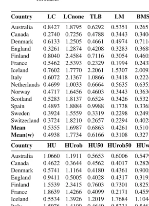
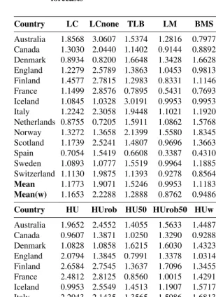
In demography, mortality rate forecasts are primarily of value for a much longer hori-zon, since the modeling error becomes the dominant error source. Therefore, we also consider ten-step-ahead forecasts. Tables 6 and 7 provide summaries of the point forecast accuracy based on the MAFEs for the ten-step-ahead forecasts of life expectancies. The summaries given in Tables 6 and 7 are averaged over different ages from 0 to 104, and years in the forecasting period (that is 11 years) for female and male data, respectively. As measured by the weighted averages of MAFEs over the fourteen countries, the LM method produces the most accurate point forecasts for both female and male data. The performance of the LM method is followed closely by the RWD method.
Figure 1: MAFEs and MFEs for the one-step-ahead point forecasts of the life expectancies by sex and method
(a) MAFEs averaged over years in the forecasting period and countries
0 20 40 60 80 100
0.0 0.5 1.0 1.5 Female Age MAFE LC LCnone TLB LM BMS HU HUrob HU50 HUrob50 HUw RWD ETS ARIMA RW
(b) MAFEs averaged over years in the forecasting period and countries
0 20 40 60 80 100
0.0 0.5 1.0 1.5 Male Age MAFE LC LCnone TLB LM BMS HU HUrob HU50 HUrob50 HUw RWD ETS ARIMA RW
(c) MFEs averaged over years in the forecasting period and countries
0 20 40 60 80 100
−0.5 0.0 0.5 1.0 1.5 Female Age MFE LC LCnone TLB LM BMS HU HUrob HU50 HUrob50 HUw RWD ETS ARIMA RW
(d) MFEs averaged over years in the forecasting period and countries
0 20 40 60 80 100
Table 6: Point forecast accuracy of the female life expectancies by method and country, as measured by the MAFEs for the ten-step-ahead forecasts
Country LC LCnone TLB LM BMS RWD RW
Australia 0.8427 1.8795 0.6292 0.5351 0.2651 0.6278 1.5353 Canada 0.2740 0.7256 0.4788 0.3443 0.3404 0.3759 0.8764 Denmark 0.6133 1.2505 0.4661 0.4974 0.7114 0.4774 0.9272 England 0.3261 1.2874 0.4208 0.3283 0.3688 0.2883 1.1776 Finland 0.8040 2.4584 0.7116 0.3054 0.4603 0.6086 1.4833 France 0.5462 2.5393 0.2329 0.1994 0.2438 0.4963 1.2108 Iceland 0.7602 1.7770 2.2061 1.5307 2.0093 0.4306 1.0592 Italy 0.6072 2.1367 1.0866 0.3418 0.2224 0.4772 1.4581 Netherlands 0.4699 1.0033 0.6664 0.5635 0.6355 0.4822 0.5167 Norway 0.4717 1.6456 0.4603 0.3443 0.3636 0.4714 1.0508 Scotland 0.5283 1.8137 0.6524 0.3426 0.5321 0.5071 1.1398 Spain 0.4893 1.8884 0.9988 0.1738 0.3368 0.4404 1.1942 Sweden 0.3924 1.5559 0.3319 0.2298 0.2492 0.4319 0.9243 Switzerland 0.3724 1.8210 0.2657 0.2294 0.4028 0.2915 1.1443
Mean 0.5355 1.6987 0.6863 0.4261 0.5101 0.4576 1.1213
Mean(w) 0.4938 1.7734 0.6166 0.3108 0.3271 0.4384 1.1883
Country HU HUrob HU50 HUrob50 HUw ETS ARIMA
Australia 1.0660 1.1911 0.5653 0.6006 0.5479 0.4665 0.6333 Canada 0.4622 0.3644 0.4562 0.4017 0.2820 0.4520 0.3825 Denmark 0.5741 1.1164 0.4180 0.4361 0.9005 0.5788 0.4448 England 0.9411 0.5005 0.4028 0.4317 0.3193 0.3462 0.3291 Finland 1.5539 2.3415 0.7603 0.7301 0.8253 0.5277 0.6582 France 1.8639 1.4266 0.4099 0.2171 0.4559 0.2511 0.4609 Iceland 0.5534 1.3926 1.2019 1.7684 1.1044 0.6355 0.5732 Italy 1.5976 1.4109 0.4649 0.5231 0.5463 0.5155 0.6599 Netherlands 0.3907 0.5530 0.6753 0.5700 0.4534 0.5378 0.6759 Norway 1.4951 1.1619 0.5021 0.8119 0.7560 0.4478 0.4552 Scotland 1.3979 1.5942 0.6322 0.6563 0.4707 0.3487 0.5731 Spain 1.0624 0.4387 0.2806 0.7619 0.3511 0.4942 0.5231 Sweden 1.0899 2.2663 0.2335 0.1900 0.5762 0.9749 0.2712 Switzerland 0.8316 0.9954 0.1447 0.4171 0.2595 0.3988 0.3542
Mean 1.0628 1.1967 0.5105 0.6083 0.5606 0.4983 0.4996
Table 7: Point forecast accuracy of the male life expectancies by method and country, as measured by the MAFEs for the ten-step-ahead forecasts
Country LC LCnone TLB LM BMS RWD RWF
Australia 1.8568 3.0607 1.5374 1.2816 0.7977 1.4248 2.0912 Canada 1.3030 2.0440 1.1402 0.9144 0.8892 1.0226 1.5626 Denmark 0.8934 0.8200 1.6648 1.3428 1.6628 0.8759 1.3720 England 1.2279 2.5789 1.3863 1.0453 0.9813 1.0087 1.7481 Finland 1.4577 2.7815 1.2983 0.8331 1.1146 1.1318 1.7642 France 1.1499 2.8576 0.7895 0.5431 0.7693 1.0279 1.4964 Iceland 1.0845 1.0328 3.0191 0.9953 0.9953 0.7207 1.2171 Italy 1.2242 2.3058 1.9448 1.1021 1.1920 0.9783 1.7411 Netherlands 0.8755 0.7205 1.5911 1.0862 1.5768 0.7231 1.2554 Norway 1.3272 1.3658 2.1399 1.5580 1.8345 1.1879 1.6232 Scotland 1.1739 2.5241 1.4807 0.9696 1.3663 1.0562 1.5450 Spain 0.7054 1.5419 0.6608 0.3387 0.4310 0.3573 1.1902 Sweden 1.0893 1.0777 1.5519 0.9964 1.1885 1.0618 1.4630 Switzerland 1.1130 1.9875 1.1393 0.9278 0.8564 0.8531 1.7434
Mean 1.1773 1.9071 1.5246 0.9953 1.1183 0.9593 1.5581
Mean(w) 1.1653 2.2288 1.2888 0.8762 0.9486 0.9341 1.5859
Country HU HUrob HU50 HUrob50 HUw ETS ARIMA
Australia 1.9652 2.4552 1.4055 1.5633 1.4487 0.8326 1.1702 Canada 0.9607 1.3871 1.0250 1.3290 0.9288 0.7481 0.7653 Denmark 1.0828 1.0858 1.6215 1.6030 1.4323 0.9687 0.8955 England 2.0794 1.3845 0.7991 1.3378 1.0314 0.9339 1.1342 Finland 2.6584 2.7545 1.3637 1.7096 1.3455 1.8616 1.7526 France 2.4812 2.8125 0.8560 1.0015 1.4291 1.5060 1.5251 Iceland 0.9953 2.5549 1.4513 1.1907 1.5717 1.6221 1.1523 Italy 2.2943 2.1435 1.3565 1.5986 1.6813 1.6645 1.9527 Netherlands 0.9503 0.9904 1.4583 1.5820 1.1502 1.3367 0.7339 Norway 1.4540 1.2805 1.4270 1.9955 1.5826 1.6695 1.2252 Scotland 2.0713 2.1025 1.6112 1.6043 1.7636 1.2111 1.2059 Spain 1.1940 0.5767 0.7037 0.8567 0.4680 1.0242 0.7571 Sweden 1.6559 1.5496 1.4764 1.6733 1.4919 1.5196 1.4889 Switzerland 1.5367 1.9608 1.2052 1.2995 1.1070 0.7689 0.9480
Mean 1.6700 1.7885 1.2686 1.4532 1.3166 1.2620 1.1933
Table 8: Forecast bias of the female life expectancies by method and country, as measured by the MFEs for the ten-step-ahead forecasts
Country LC LCnone TLB LM BMS RWD RW
Australia 0.7461 1.8297 0.5354 0.4789 0.0745 0.6231 1.5257 Canada -0.0022 0.6818 -0.4709 -0.2244 -0.1916 -0.2125 0.8516 Denmark 0.0600 1.2505 -0.2649 0.0717 0.2539 0.3115 0.9262 England 0.2704 1.2870 0.3737 0.2627 0.2957 0.1555 1.1742 Finland 0.6991 2.4227 0.5530 0.1690 0.0914 0.5394 1.4740 France 0.4506 2.5393 0.1419 -0.1025 -0.0215 0.4800 1.2101 Iceland 0.7201 1.7502 2.1932 1.4099 1.9936 0.1450 1.0164 Italy 0.5788 2.1247 1.0859 0.3239 0.1747 0.3267 1.4574 Netherlands -0.1837 0.9809 -0.6664 -0.4914 -0.5953 -0.3166 0.4947 Norway 0.3034 1.6309 0.3886 0.2220 0.2424 0.4194 1.0254 Scotland 0.3762 1.8137 0.3408 0.1059 0.3288 0.4652 1.1312 Spain 0.2796 1.7999 0.9533 0.0586 0.2310 -0.1648 1.1925 Sweden 0.2604 1.5438 -0.3160 -0.1833 -0.0537 0.4240 0.9233 Switzerland 0.1466 1.7982 -0.0046 -0.1222 -0.2915 -0.0235 1.1388
Mean 0.3361 1.6752 0.3459 0.1413 0.1809 0.2266 1.1101
Mean(w) 0.3441 1.7493 0.3779 0.0799 0.0761 0.1949 1.1823
Country HU HUrob HU50 HUrob50 HUw ETS ARIMA
Australia 0.9872 1.1629 0.4613 0.5290 0.5229 0.4665 0.6256 Canada -0.3297 -0.1349 -0.4199 -0.2882 -0.1078 0.4520 -0.2493 Denmark 0.5704 1.1032 -0.0748 0.2442 0.8964 0.5788 0.1803 England 0.9256 0.4594 0.1718 0.3208 0.2123 0.3462 0.2373 Finland 1.5070 2.2997 0.6055 0.6481 0.7753 0.5277 0.5569 France 1.8415 1.4219 -0.1972 -0.0513 0.4271 0.2511 0.3894 Iceland 0.3473 1.3218 1.1449 1.7500 1.0699 0.6355 0.2124 Italy 1.5930 1.4079 0.1318 0.3938 0.5167 0.5155 0.4323 Netherlands 0.3356 0.4204 -0.6649 -0.5309 -0.1154 0.5378 -0.5382 Norway 1.4469 1.0662 0.4369 0.7788 0.6955 0.4478 0.3881 Scotland 1.3923 1.5872 0.3941 0.3051 0.3567 0.3487 0.5378 Spain 0.9856 0.4067 0.1763 0.6476 0.2069 0.4942 -0.1940 Sweden 1.0752 2.1968 -0.2323 0.0510 0.5627 0.9749 0.2355 Switzerland 0.8144 0.9586 -0.0436 0.3457 0.1308 0.3988 -0.1595
Mean 0.9637 1.1198 0.1350 0.3674 0.4393 0.4983 0.1896
Table 9: Forecast bias of the male life expectancies by method and country, as measured by the MFEs for the ten-step-ahead forecasts
Country LC LCnone TLB LM BMS RWD RWF
Australia 1.3904 2.9052 1.4429 1.2240 0.6932 1.4222 2.0825 Canada 1.1552 1.9571 1.0852 0.8829 0.8262 0.9950 1.5425 Denmark 0.8934 0.8121 1.5553 1.1867 1.6276 0.8551 1.3569 England 1.2279 2.5789 1.3648 1.0268 0.9388 0.9965 1.7432 Finland 1.4131 2.7807 1.1515 0.6600 0.4264 1.1086 1.7515 France 1.1428 2.8564 0.7538 0.5087 0.7241 1.0278 1.4947 Iceland 0.9191 0.8624 2.4072 2.5259 1.2828 0.5849 0.9191 Italy 1.2157 2.3049 1.9108 1.0595 1.1492 0.9497 1.7365 Netherlands 0.8609 0.6971 1.4517 1.0030 1.4563 0.6703 1.2255 Norway 1.3011 1.3428 2.1088 1.4685 1.8153 1.1418 1.5836 Scotland 1.1585 2.5241 1.3961 0.8820 -0.0818 1.0537 1.5445 Spain 0.1861 1.2384 0.6478 0.2853 0.4140 0.2250 1.1847 Sweden 1.0862 1.0747 1.4730 0.9248 1.0749 1.0536 1.4557 Switzerland 1.0088 1.9324 1.0902 0.8707 0.7514 0.8272 1.7318
Mean 1.0685 1.8477 1.4171 1.0363 0.9356 0.9222 1.5252
Mean(w) 1.0439 2.1661 1.2426 0.8297 0.8645 0.9012 1.5775
Country HU HUrob HU50 HUrob50 HUw ETS ARIMA
Australia 1.7630 2.4491 1.3151 1.4997 1.4056 0.8326 1.1602 Canada 0.8888 1.3001 0.9715 1.2835 0.8884 0.7481 0.7297 Denmark 1.0816 1.0647 1.5559 1.5659 1.4253 0.9687 0.8585 England 2.0634 1.3287 0.7883 1.3095 0.9811 0.9339 1.1254 Finland 2.6579 2.6568 1.2331 1.5355 1.3272 1.8616 1.7372 France 2.4310 2.8095 0.8343 0.9658 1.4220 1.5060 1.5236 Iceland 1.0756 1.0646 2.0222 1.3571 1.4979 1.6221 1.0992 Italy 2.2758 2.1431 1.3270 1.5572 1.6715 1.6645 1.8509 Netherlands 0.9432 0.9121 1.3293 1.5016 1.1315 1.3367 0.5153 Norway 1.4192 1.1604 1.3888 1.9328 1.5347 1.6695 1.2007 Scotland 2.0713 2.0972 1.5541 1.5741 1.7622 1.2111 1.2023 Spain 1.0824 0.5506 0.6500 0.7439 0.3435 1.0242 0.6774 Sweden 1.6555 1.5401 1.3986 1.5825 1.4764 1.5196 1.4823 Switzerland 1.5106 1.9238 1.1533 1.2370 1.0544 0.7689 0.9257
Mean 1.6371 1.6429 1.2515 1.4033 1.2801 1.2620 1.1492
Figures 2a and 2b show the MAFEs of the ten-step-ahead point forecasts for different methods. The MAFEs are averaged over countries and years in the forecasting period for the female and male life expectancies. Large errors occur between ages 0 and 60 for most of the methods, and errors from the LCnone, HU, HUrob and RW methods are particularly large at these ages. At older ages11, the MAFEs of all methods decrease
gradually. For ages above 100, there is a sharp increase in MAFEs, which reflects the difficulty in forecasting the mortality rates at old ages because of excessive variability.
Figure 2: MAFEs and MFEs for the ten-step-ahead point forecasts of the life expectancies by sex and method
(a) MAFEs averaged over years in the forecasting period and countries
0 20 40 60 80 100
0.0 0.5 1.0 1.5 2.0 Female Age MAFE LC LCnone TLB LM BMS HU HUrob HU50 HUrob50 HUw RWD ETS ARIMA RW
(b) MAFEs averaged over years in the forecasting period and countries
0 20 40 60 80 100
0.0 0.5 1.0 1.5 2.0 2.5 Male Age MAFE LC LCnone TLB LM BMS HU HUrob HU50 HUrob50 HUw RWD ETS ARIMA RW
Figures 1c and 1d show the MFEs of the ten-step-ahead point forecasts for different methods. The MFEs are averaged over countries and years in the forecasting period for the female and male life expectancies. In the female data, apart from the LC, RW and two univariate time-series methods, all other methods underestimate life expectancies from ages 0 to 65, and the degree of underestimation becomes smaller and smaller as age increases. The LM and RWD methods perform similarly, but they are both more superior to the LC method.
Figure 2: (Continued)
(c) MFEs averaged over years in the forecasting period and countries
0 20 40 60 80 100
−1 0 1 2 Female Age MAFE LC LCnone TLB LM BMS HU HUrob HU50 HUrob50 HUw RWD ETS ARIMA RW
(d) MFEs averaged over years in the forecasting period and countries
0 20 40 60 80 100
−1 0 1 2 Male Age MAFE LC LCnone TLB LM BMS HU HUrob HU50 HUrob50 HUw RWD ETS ARIMA RW
7.
Comparisons of the interval forecasts
As was emphasized by Chatfield (1993, 2000), it is important to provide interval forecasts as well as point forecasts, so as to (1) assess future uncertainty level, (2) enable differ-ent strategies to be planned for the range of possible outcomes indicated by the interval forecasts, (3) compare forecasts from different methods more thoroughly, and (4) explore different scenarios based on different assumptions.
In recent years, many authors have provided interval forecasts to measure the uncer-tainty associated with the point forecasts; see for example, Lutz and Scherbov (1998) for Austria, Alho (1998) for Finland, Keilman and Pham (2000) for Norway, and Tayman, Smith, and Lin (2007) for the United States. These methods have been motivated by earlier work on stochastic forecasts, by for instance, Lee (1974), Stoto (1983), Alho and Spencer (1985), Alho (1990) and Lee and Tuljapurkar (1994). The current paper is a contribution to the literature in this area.
Rowland 2003, Chapter 8 for detail). Prediction interval was customarily constructed by 80% percentile of the simulated sets of the life expectancies.
Table 10: Coverage probability deviances of the one-step-ahead forecast female life expectancies by method and country. Minus sign indi-cates that the empirical coverage probability is less than the nomi-nal coverage probability
Country LC LCnone TLB LM BMS RWD RW
Australia 0.2500( – ) 0.7929( – ) 0.4048( – ) 0.1243( – ) 0.0324( – ) 0.1790(+) 0.1162(+) Canada 0.2624( – ) 0.7881( – ) 0.4800( – ) 0.0714( – ) 0.3081( – ) 0.1929(+) 0.1648(+) Denmark 0.6519( – ) 0.7595( – ) 0.2648( – ) 0.2519( – ) 0.5181( – ) 0.2000(+) 0.1995(+) England 0.1086( – ) 0.7929( – ) 0.5086( – ) 0.1805( – ) 0.1957( – ) 0.1890(+) 0.1805(+) Finland 0.5433( – ) 0.7881( – ) 0.6390( – ) 0.0443( – ) 0.1267( – ) 0.1819(+) 0.1667(+) France 0.5824( – ) 0.8000( – ) 0.3167( – ) 0.0824( – ) 0.1333( – ) 0.1752(+) 0.1729(+) Iceland 0.0629( – ) 0.6476( – ) 0.6776( – ) 0.5843( – ) 0.7248( – ) 0.2000(+) 0.2000(+) Italy 0.4319( – ) 0.7943( – ) 0.7648( – ) 0.1300( – ) 0.1243( – ) 0.1757(+) 0.1729(+) Netherlands 0.3414( – ) 0.7514( – ) 0.3938( – ) 0.1457( – ) 0.2595( – ) 0.2000(+) 0.2000(+) Norway 0.6881( – ) 0.7890( – ) 0.3481( – ) 0.2505( – ) 0.2924( – ) 0.1938(+) 0.1900(+) Scotland 0.6238( – ) 0.7890( – ) 0.4395( – ) 0.1576( – ) 0.1519( – ) 0.1648(+) 0.1643(+) Spain 0.5390( – ) 0.7981( – ) 0.7981( – ) 0.2362( – ) 0.3700( – ) 0.1971(+) 0.1924(+) Sweden 0.5667( – ) 0.7824( – ) 0.2471( – ) 0.1810( – ) 0.2419( – ) 0.2000(+) 0.2000(+) Switzerland 0.4100( – ) 0.7795( – ) 0.0919( – ) 0.1095( – ) 0.1648( – ) 0.1948(+) 0.1810(+)
Mean 0.4330( – ) 0.7752( – ) 0.4553( – ) 0.1821( – ) 0.2603( – ) 0.1889(+) 0.1787(+)
Mean(w) 0.3983( – ) 0.7918( – ) 0.5205( – ) 0.1432( – ) 0.2042( – ) 0.1858(+) 0.1754(+)
Country HU HUrob HU50 HUrob50 HUw ETS ARIMA
Australia 0.2000(+) 0.0119( – ) 0.1981(+) 0.0152(+) 0.2000(+) 0.1867(+) 0.1767(+)
Canada 0.2000(+) 0.2000(+) 0.2000(+) 0.1990(+) 0.2000(+) 0.1667(+) 0.1433(+)
Denmark 0.2000(+) 0.1343(+) 0.1890(+) 0.1819(+) 0.2000(+) 0.1757(+) 0.1857(+)
England 0.1981(+) 0.1538(+) 0.1362(+) 0.0548( – ) 0.2000(+) 0.1490(+) 0.1562(+) Finland 0.2000(+) 0.2614( – ) 0.1557(+) 0.0962(+) 0.2000(+) 0.1795(+) 0.1681(+) France 0.0395(+) 0.1143( – ) 0.1476(+) 0.1343(+) 0.2000(+) 0.1776(+) 0.1710(+)
Iceland 0.2000(+) 0.2000(+) 0.2000(+) 0.2000(+) 0.2000(+) 0.2000(+) 0.2000(+)
Italy 0.1438(+) 0.0590(+) 0.1500(+) 0.0700(+) 0.2000(+) 0.1795(+) 0.1743(+)
Netherlands 0.2000(+) 0.2000(+) 0.1110(+) 0.1948(+) 0.2000(+) 0.1995(+) 0.1971(+) Norway 0.0671( – ) 0.0919(+) 0.1667(+) 0.1038(+) 0.2000(+) 0.1548(+) 0.1471(+) Scotland 0.1129(+) 0.3705( – ) 0.1200(+) 0.1643(+) 0.2000(+) 0.1714(+) 0.1886(+)
Spain 0.1976(+) 0.2000(+) 0.1719(+) 0.0300( – ) 0.2000(+) 0.1952(+) 0.1938(+)
Sweden 0.2000(+) 0.5748( – ) 0.1976(+) 0.1862(+) 0.2000(+) 0.2000(+) 0.2000(+) Switzerland 0.2000(+) 0.1576(+) 0.2000(+) 0.1767(+) 0.2000(+) 0.1548(+) 0.1790(+)
Mean 0.1685(+) 0.1950(+) 0.1674(+) 0.1291(+) 0.2000(+) 0.1779(+) 0.1772(+)
Table 11: Coverage probability deviance of the one-step-ahead forecast male life expectancies by method and country. Minus sign indicates that the empirical coverage probability is less than the nominal coverage probability
Country LC LCnone TLB LM BMS RWD RW
Australia 0.4329( – ) 0.7929( – ) 0.6867( – ) 0.2305( – ) 0.1886( – ) 0.1457(+) 0.0824(+) Canada 0.6452( – ) 0.7805( – ) 0.7629( – ) 0.4471( – ) 0.6957( – ) 0.1267(+) 0.0533(+) Denmark 0.4886( – ) 0.6138( – ) 0.6433( – ) 0.4943( – ) 0.6471( – ) 0.2000(+) 0.1995(+) England 0.4219( – ) 0.8000( – ) 0.7400( – ) 0.2271( – ) 0.2610( – ) 0.1724(+) 0.1348(+) Finland 0.3605( – ) 0.7686( – ) 0.5333( – ) 0.0767( – ) 0.2171( – ) 0.1910(+) 0.1862(+) France 0.5086( – ) 0.7933( – ) 0.3367( – ) 0.0714( – ) 0.3681( – ) 0.1824(+) 0.1800(+) Iceland 0.0981( – ) 0.2081( – ) 0.6410( – ) 0.3011( – ) 0.7257( – ) 0.2000(+) 0.2000(+) Italy 0.4419( – ) 0.7895( – ) 0.7552( – ) 0.2876( – ) 0.4752( – ) 0.1857(+) 0.1833(+) Netherlands 0.0690( – ) 0.2676( – ) 0.7729( – ) 0.5052( – ) 0.7524( – ) 0.1981(+) 0.1981(+) Norway 0.4738( – ) 0.6490( – ) 0.7771( – ) 0.5357( – ) 0.5419( – ) 0.1467(+) 0.1395(+) Scotland 0.7248( – ) 0.7995( – ) 0.5852( – ) 0.3195( – ) 0.3119( – ) 0.1562(+) 0.1452(+) Spain 0.4771( – ) 0.7500( – ) 0.6086( – ) 0.1767( – ) 0.4595( – ) 0.1943(+) 0.1919(+) Sweden 0.1571( – ) 0.3500( – ) 0.7329( – ) 0.3062( – ) 0.4600( – ) 0.2000(+) 0.2000(+) Switzerland 0.3057( – ) 0.7248( – ) 0.3329( – ) 0.2367( – ) 0.3105( – ) 0.1714(+) 0.1671(+)
Mean 0.4004( – ) 0.6491( – ) 0.6363( – ) 0.3011( – ) 0.4582( – ) 0.1765(+) 0.1615(+)
Mean(w) 0.4494( – ) 0.7412( – ) 0.6357( – ) 0.2485( – ) 0.4250( – ) 0.1754(+) 0.1557(+)
Country HU HUrob HU50 HUrob50 HUw ETS ARIMA
Australia 0.1286(+) 0.0881( – ) 0.1133(+) 0.1581( – ) 0.2000(+) 0.1462(+) 0.1110(+) Canada 0.0429( – ) 0.3033( – ) 0.0295( – ) 0.2205( – ) 0.2000(+) 0.1200(+) 0.1276(+) Denmark 0.0967(+) 0.0638(+) 0.0300( – ) 0.0757( – ) 0.2000(+) 0.1029(+) 0.1162(+) England 0.0786( – ) 0.2043( – ) 0.0724( – ) 0.3738( – ) 0.2000(+) 0.1352(+) 0.0814(+) Finland 0.0700(+) 0.2781( – ) 0.1386(+) 0.0871( – ) 0.2000(+) 0.1738(+) 0.1695(+) France 0.1881( – ) 0.3529( – ) 0.0733(+) 0.0129( – ) 0.2000(+) 0.1805(+) 0.1738(+)
Iceland 0.1995(+) 0.2000(+) 0.2000(+) 0.2000(+) 0.2000(+) 0.1967(+) 0.2000(+)
Italy 0.0205(+) 0.2729( – ) 0.0305(+) 0.1176( – ) 0.2000(+) 0.1848(+) 0.1629(+) Netherlands 0.0662(+) 0.2000(+) 0.2305( – ) 0.2657( – ) 0.1971(+) 0.1800(+) 0.1810(+)
Norway 0.1171(+) 0.1205(+) 0.0238(+) 0.3157( – ) 0.2000(+) 0.0929(+) 0.0729(+)
Scotland 0.1576( – ) 0.3081( – ) 0.1686( – ) 0.1867( – ) 0.2000(+) 0.1176(+) 0.0467(+)
Spain 0.1905(+) 0.2000(+) 0.0495(+) 0.1157(+) 0.2000(+) 0.1914(+) 0.1910(+)
Sweden 0.2000(+) 0.0281( – ) 0.1495( – ) 0.3300( – ) 0.1990(+) 0.1986(+) 0.1900(+) Switzerland 0.1119(+) 0.2738( – ) 0.1776(+) 0.1695(+) 0.2000(+) 0.1419(+) 0.1257(+)
Mean 0.1191(+) 0.2067(-) 0.1062(+) 0.1878(-) 0.1997(+) 0.1545(+) 0.1393(+)