Implement and Test Algorithm Finding Maximal Flow Limited Cost in Extended Multi commodity Multicost Network

(1)

ISSN : 2394-2231 http://www.ijctjournal.org Page 1

Implement and Test Algorithm Finding Maximal Flow

Limited Cost in Extended Multi commodity Multicost

Network

Ho Van Hung

1

and Tran Quoc Chien

2

1_{Quangnam University, Tamky, Vietnam}

2_{The University of Education, University of Danang, Danang, Vietnam}

Abstract:

Graph is a powerful mathematical tool applied in many fields as transportation, communication, informatics, economy,… In ordinary graph the weights of edges and vertexes are considered independently where the length of a path is the sum of weights of the edges and the vertexes on this path. However, in many practical problems, weights at a vertex are not the same for all paths passing this vertex, but depend on coming and leavingedges. Furthermore, on a network, many commodities share capacities of edges and vertexes with different costs. So it is necessary to study network with mutiple weights. The presented paper introduces the algorithm to find the shortest path between two vertices on extended graph with mutiple weights. Then, the shortest path finding algorithms is used to implement the general algorithm finding the maximum flow limited cost on the extended multicommodity multicost network developed in the article[14].

Keywords: Graph, Network, Multicommodity Multicost Flow, Optimization, Linear Programming.

1. Introduction

Network and its flow is a powerful mathematical tool applied in many fields as transportation, communications, informatics, economics, and so on. So far, most of applications in graphsjust solely consider to the weights of edges and nodes independently, in which the path length merely is the sum ofweights of edges and nodes along the path. However, in many practical problems, the weight ata node is not the same for all paths passing through that node, but also depends on coming and leaving edges. For example, the transit time on the transport network depends on the direction of transportation: turn right, turn left or go straight, even some directions areforbidden. Paper [2] propose switching cost only for directed graphs. Multicommodity flow in traditional network problems have been studied in the papers [1,3,4,5,6]. Multicommodity flow in extended network problems with extended transport networks were studied in the papers [7-11].Furthermore, on a network, many commodities share capacities of edges and vertexes with different costs. So it is necessary to study network with mutiple weights. The paper [12] and [13] study maximal flow problems and the paper [14] studies maximal flow limited cost problems on extended multicommodity multicost networks.

The presented paper introduces the algorithm to find the shortest path between two vertices on extended graph with mutiple weights. Then, the shortest path finding algorithms is used to implement the general algorithm finding the maximum flow limited cost on the extended multicommodity multicost network developed in the

article [14]. The content of the paper is as follows. The maximal flow limited cost problems on extended multicommodity multicost networks is introduced in section 2. In section 3, the shortest path finding algorithms is used to implement the general algorithm finding the maximum flow limited cost on the extended multicommodity multicost network developed in the article [14]. The algorithm is coded in the programming language C and tested in section 4.

2. Maximal Flow Limited Cost Problems In

Extended

Multicommodity

Multicost

Network

Given mixed graph G = (V, E)with node set V and edge set E. The edges may be undirected or directed. The symbol Evis the set of edges incident verticev∈V. There

are many kinds of goods circulating on the network. Commodities share the capacities of the edges, but have different costs. The undirected edges represent the two-way edge, in which the goods on the same edge, but reverse directions share the capacity of the edge. The symbol r is the commodity number,qi> 0 is the

coefficient of conversion of commodityi, i =1..r. Given the following functions:

Edge passing capacity function ce:E→R*, where ce(e)is the passing capabilityof theedge e∈E.

Edge service coefficientfunction ze:E→R*, where ze(e)is the passingratio of the edge e∈E (the real capacity of the edge e is ze(e).ce(e)).

(2)

ISSN : 2394-2231 http://www.ijctjournal.org Page 2

Node service coefficient function zv:V→R*, wherezv(u) is the passingratio of the node v∈V (the real capacity of the node v is zv(v).cv(v)).

The tuples (V,E, ce, ze, cv, zv) arecalledextended networks.

Edge cost function i, i=1..r,bei:E→R*, where bei(e) is the

cost of passing e a converted unit of commodity of type

i. Note that with 2-waypaths, the costs of each way may vary.

Node switch cost function i, i=1..r,bvi:V×Ev×Ev→R*,

where bvi(u,e,e’) is the cost of transferring a converted

unit of commodity of typei from edge e through u to edge e’.

The sets ((V, E, ce, ze, cv, zv,{bei,bvi, qi|i=1..r}) are

calledthe extended linear multicommodity multicost network.

◊Note:

If bei(e)=∞, commodity of type iis prohibited from

circulation on pathe. If bvi(u,e,e’) = ∞,comodity of type

iis banned from pathe through u to pathe’.

Let p be the path from node u to node v through edges ej,

j=1..(h+1), and nodes uj, j=1..has follows

p = [u, e1, u1, e2, u2, …, eh, uh, eh+1, v] (1) The cost of circulating a converted unit of commodity of type i, i = 1..r, passing the path p, is denoted by the symbol bi(p), and definedby the following formula:

bi(p) =

∑

+ = 1 1

)

(

h j j i

e

be

+

∑

= + h j j j j

i

u

e

bv

1

)

,

(

(2)

Given a multicost multicommodity networkG=(V,E,ce, ze, cv, zv, {bei, bvi, qi|i=1..r}). Assume, for each

commodityof typei, i=1..r, there arekisource-target pairs

(si,j, ti,j), j=1..ki, each pair assigned a quantity of

commodity of type i, that is necessary to move from source node si,j to target node ti,j.

DenotePi,j is the set of paths from node si,j to node ti, in

G, which commodity of type i can be passed,i=1..r,j=1..ki. Set

Pi=

U

i k j j i

P

1 , =

. (3)

For each pathp

∈

Pi,j, i=1..r, j=1..ki, denotexi,j(p) the flow

of converted commodity of type i from the source nodesi,jto the destination nodeti,j along the pathp, i=1..r,

j=1..ki.

DenotePi,ethe set of paths in Pipassing through the edge

e, ∀e∈E.

Denote Pi,vthe set of paths in Pipassing through the node

v, ∀v∈V. A set

F = {xi,j(p) | p

∈

Pi,j,i=1..r,j=1..ki} (4)

is called amulticommodity flow on the linear extended multicommodity multicost network, if it satisfies the following edge and node capacity constraints:

( )

∑∑ ∑

= = ∈ r i k

j p P

j i i e i

p

x

1 1 , ,

≤ce(e).ze(e), ∀e∈E (5)

( )

∑∑ ∑

= = ∈ r i k

j p P

j i i v i

p

x

1 1 , ,

≤cv(v).zv(v), ∀v∈V (6)

The expressions

fvi,j =

∑

( )

∈Pij p

j i

p

x

,

, ,i=1..r,j=1..ki (7)

is calledthe flow value of commodity of type i of the source-target pair (si,j,ti,j) of F.

The expresstions

fvi =

∑

= i k j j i

fv

1

, , i=1..r (8) is called the flow value of commodity of type i of F. The expresstion

fv =

∑

= r i i

fv

1 (9)

is called the flow value of F.

Given an extended linearmulticommodity multicost networkG=(V,E, ce, ze, cv, zv, {bei, bvi, qi|i=1..r}).

Assume, for each commodity of type i, i=1..r, there are

ki source-target pairs (si,j, ti,j), j=1..ki, each pair assigned a

quantity of comodity of type i, that is necessary to move from source node si,j to target node ti,j.Given a limit

costB.

The task of the problem is to find the multicommodity flow such that the value of the flow fvis maximal. At the same time, the total cost of the flow does not exceed B.

The problem is expressed by the an implicit linear programming model (P) as follows:

fv=

∑∑ ∑

= = ∈

r

i k

j p P j i i j i

p

x

1 1 , ,

)

(

→max

satisfies

( )

∑∑ ∑

= = ∈ r i k

j p P

j i i e i

p

x

1 1 , ,

≤ce(e).ze(e), ∀e∈E

( )

∑∑ ∑

= = ∈ r i k

j p P

j i i v i

p

x

1 1 , ,

≤cv(v).zv(v), ∀v∈V

(P)

( )

.

(

)

1 1 , ,

p

b

p

x

i r i k

j p P j i i j i

∑∑ ∑

= = ∈ ≤B

xi,j(p) ≥0, ∀i=1..r, j=1..ki, ∀p

∈

Pi,j

(3)

ISSN : 2394-2231 http://www.ijctjournal.org Page 3

The general algorithm with polynomial complexity is

proved in [14]. In this paper we integrate the algorithm finding shortest path [7,8] in order to implement the mentioned algorithm [14].

3.1. The problem of finding the shortest path in extended graph

Given extended mixed graph G = (V, E) with a set of vertices V and a set of edges E, where edges can be directed or undirected. Each edge e∈E is assigned a

weight we(e). For each vertex v∈V, we denote Ev the set

of edges incident vertex v. For each vertex v∈V and each of pair of edges(e,e’)∈Ev×Ev, e≠e’ is assigned

switch weight wv(v,e,e’).

The sets (V, E, we, wv) are called extended graph. Let p be a path from a vertex u to a vertex v

through the edges ei, i = 1, …, h+1, and vertices ui, i = 1,

…, h, as following:

p = [u, e1, u1, e2, u2, …, eh, uh, eh+1, v] (10) Define the length of the path p, denoted l(p), as following:

l(p) =

∑

+

=

1

)

(

h

j

e

we

+

∑

=

+ h

j

j j j

e

u

wv

1

)

,

(

(11)

•The problem of finding the shortest path

Given extended graph G = (V, E, we, wv) and vertices s,

t∈V . Find the shortest path from s to t.

The following function find the shortest path p from s to

tand return the length of p. This function uses the following notations:

S is a set of the vertices that found the shortest path starting from s;

T = V - S;

l(v) is the length of the shortest path from s to v;

le(v) is the edge that leads to the vertex v on the shortest path from s to v;

VE = {(v,e) | v∈V−{s} &e∈Ev}∪{(s,∅)} is the

set of pairs of vertices and incident edges;

SE is a set of vertex-edge excluded from VE;

TE = VE - SE;

L(v, e) is the label of the vertex-edge pair (v,e)∈VE

P(v, e) is the vertex-edge adjacent before (v,e)∈VE.

float ShortestPath(V,E,we,wv,s,t,p) {

// Initialization

S = ∅ ; T = V ;

VE={(v,e)|v∈V−{s}&e∈Ev}∪{(s,∅)};

SE = ∅; TE = VE;

L(v,e)=+∞;∀(v,e)∈VE, L(s,∅) = 0; for (v,e)∈VE: P(v,e) = ∅;

// main algorithm body

do {

m = min{L(v,e) | (v,e)∈TE}. if (m< +∞)

{

Choose (vmin,emin)∈TE such that

L(vmin,emin) ==m;

TE = TE−{(vmin,emin)};

SE = SE∪{(vmin,emin)};

if (vmin∉S)

{

le(vmin)=emin;

S = S∪{vmin};

l(vmin)=L(vmin,emin);

T = T–{vmin};

}

if (t<>vmin)

{

for (v,e)∈TE adjacent

after (vmin,emin)

{

if (vmin==s)

L’(v,e)=L(s,∅)

+we(vmin,v);

else

L’(v,e)=L(vmin,emin)+w

e(vmin,v)+wv(vmin,emin,

e);

If(L(v,e)>L’(v,e)) {

L(v,e)=L’(v,e);

P(v,e)=(vmin,emin);

}

} }

}

} while (m< +∞ or t <>vmin)

if (m == +∞)return +∞; // no

path exists from s to t

// finding the shortest path

k=1; (vk,ek) = P(t,le(t));

while ((vk,ek) <> (s,∅))

{

k=k+1; (vk,ek) = P(vk−1,ek−1);

}

p = s→vk →vk−1→ … →v1→t

return L(t,le(t));// shortest

path length from s to t.

} // end of ShortestPath

(4)

ISSN : 2394-2231 http://www.ijctjournal.org Page 4

◊Input: Extended multicost multicommodity network

G=(V,E, ce, ze, cv, zv, {bei, bvi, qi|i=1..r}), n=|V|, m=|E|.

Assume, for each commodity of type i, i=1..r, there are

ki source-target pairs (si,j, ti,j), j=1..ki, each pair assigned a

quantity of commodity of type i, that is necessary to move from source node si,j to target node ti,j.Given a

limited cost B, an approximation ratio ω.

◊Output: Maximal flow F represents a set of converged

flows at the edges

F = {xi,j(e) | e

∈

E, i=1..r, j=1..ki}

with total costBfnot over the limit costB.

◊Procedure

// Calculatebmin, the smallest cost in the paths from the source si,j to the destination ti,j.

For (i=1..r, j=1..ki)bmin = min{bi(p) | i=1..r,

j=1..ki, p∈Pi,j}.

bmin = ∞;

for(i=1; i <= r; i++) for(j=1; i <= ki; j++)

{

l=ShortestPath(V,E,bei,bvi,sij,tij,p)

if (bmin > l) bmin = l; }

// Choosebmax>= max{bi(p) | i=1..r, j=1..ki, p∈Pi,j}. c1 = 0;

for(i=1;i<=r;i++)

for(e∈E)

if (bei(e)>c1)

c1 = bei(e);c2 = 0;

for(i=1;i<=r;i++)

for(v∈E)

for(e,e’)∈Ev×Ev

if (bvi(v,e,e’)>c2)

c2 = bvi(v,e,e’);

bmax = n*(c1+c2);

//Choose ε, δ and initialization

ε = 1−

1 /(

1 +

ω

)

;

δ = (1+ε)

[

]

ε

2 1/

min)

max/

(

)

1 (

1 b

b

n

+

;

for (e

∈

E) le(e)=δ; for (v∈V) lv(v)=δ ;

ϕ = δ/bmin ;fv=0;

Bf = 0 ;

for(i=1; i <= r; i++)

for(j=1; i <= ki; j++)

for (e

∈

E)

xi,j(e)=0 ;

// Note

imin and jminthe indexes of source-destination pairs with the shortest path;

α the shortest path length;

p the shortest path;

c the minimal edge and node capacity on the path p, i.e.

// main algorithm body

do {

α = ∞; imin = 1; jmin = 1; p = ∅;

for(i=1; i <= r; i++) for(j=1; i <= ki; j++)

{

l =

ShortestPath(V,E,le+ϕ.bei, lv+ϕ.bvi,

sij, tij, ptemp)

if (α> l) {

α = l; imin = i;

jmin = j; p = ptemp; }

}

c=min{min{ce(e).ze(e)|e∈p},min{cv(v

).zv(v)|v∈p}};

B’ = c.bimin(p);

if (B’>B){ c = c.B / B’; B’ = B; }

//Flow adjustments:

for(e

∈

p){xi,j(e)=xi,j(e)+c;le(e)=l(e).(1+ε.c/(

ce(e).ze(e)));} for

(v∈p)lv(v)=lv(v).(1+ε.c/(cv(v).zv(v)))

; ϕ = ϕ.(1+ε.B’/B) ;

Bf = Bf + B’ ;

fv = fv + c ;

} while (α<1)

// Modifying the resulting flows F and flow value fv.

for(i=1; i <= r; i++)

for(j=1; i <= ki; j++)

for (e

∈

E)

xi,j(e)=xi,j(e)/(1-log1+εδ);

fv = fv/(1-log1+εδ);

Bf = Bf/(1-log1+εδ);

// Modifyingflows on scalar edge

for(i=1; i <= r; i++)

for(j=1; i <= ki; j++)

for (e

∈

E&& e scalar) if xi,j(e)>=xi,j(e’)//e’ is the

opposite of the direction e

{

xi,j(e)=xi,j(e)−xi,j(e’);

xi,j(e’)=0

}; else

{xi,j(e’)=xi,j(e’)−xi,j(e) ;

(5)

ISSN : 2394-2231 http://www.ijctjournal.org Page 5

/*** end of algorithm ***/

4. T

EST

4.1. Example

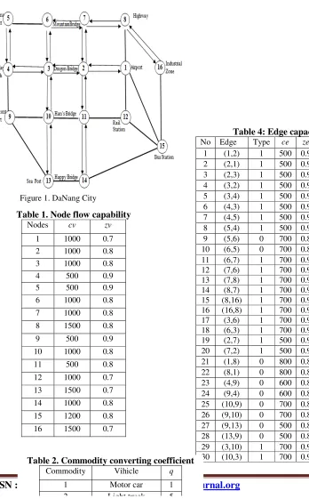
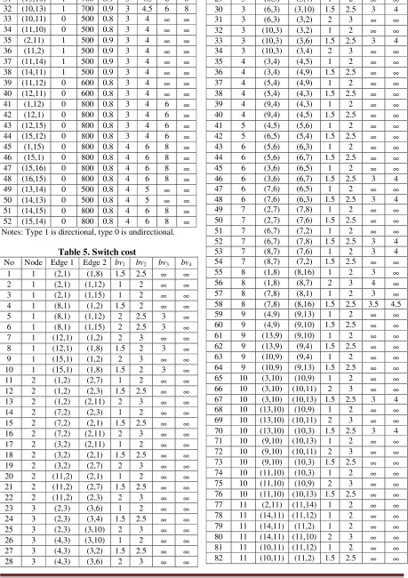
The following example is inspired by the beautiful DaNang City of VietNam, where the world leaders were welcomed to take part in the APEC 2017. The traffic network is in Figure 1. The database contains the table 1, table 2, table 3, table 4 and table 5.

Figure 1. DaNang City

Table 4: Edge capacity and cost

No Edge Type ce ze be1 be2 be3 be4 1 (1,2) 1 500 0.9 3 4 ∞ ∞

2 (2,1) 1 500 0.9 3 4 ∞ ∞

3 (2,3) 1 500 0.9 3 4 ∞ ∞

4 (3,2) 1 500 0.9 3 4 ∞ ∞

5 (3,4) 1 500 0.9 3 4 ∞ ∞

6 (4,3) 1 500 0.9 3 4 ∞ ∞

7 (4,5) 1 500 0.9 3 4 ∞ ∞

8 (5,4) 1 500 0.9 3 4 ∞ ∞

9 (5,6) 0 700 0.8 3 4 ∞ ∞

10 (6,5) 0 700 0.8 3 4 ∞ ∞

11 (6,7) 1 700 0.9 3 4 6 8 12 (7,6) 1 700 0.9 3 4 6 8 13 (7,8) 1 700 0.9 3 4 6 8 14 (8,7) 1 700 0.9 3 4 6 8 15 (8,16) 1 700 0.9 3 4 6 8 16 (16,8) 1 700 0.9 3 4 6 8 17 (3,6) 1 700 0.9 3 4 6 8 18 (6,3) 1 700 0.9 3 4 6 8 19 (2,7) 1 500 0.9 3 4 ∞ ∞

20 (7,2) 1 500 0.9 3 4 ∞ ∞

21 (1,8) 0 800 0.8 3 4 6 ∞

22 (8,1) 0 800 0.8 3 4 6 ∞

23 (4,9) 0 600 0.8 4 5 ∞ ∞

24 (9,4) 0 600 0.8 3 4 ∞ ∞

25 (10,9) 0 700 0.8 4 5 ∞ ∞

26 (9,10) 0 700 0.8 3 4 ∞ ∞

27 (9,13) 0 500 0.8 3 4 ∞ ∞

28 (13,9) 0 500 0.8 4 5 ∞ ∞

29 (3,10) 1 700 0.9 3 4.5 6 8 30 (10,3) 1 700 0.9 3 4.5 6 8 Table 2. Commodity converting coefficient

Commodity Vihicle q

1 Motor car 1

2 Light truck 5 Table 1. Node flow capability

Nodes cv zv

1 1000 0.7 2 1000 0.8 3 1000 0.8 4 500 0.9 5 500 0.9 6 1000 0.8

7 1000 0.8 8 1500 0.8

9 500 0.9

10 1000 0.8

11 500 0.8

12 1000 0.7 13 1500 0.7

14 1000 0.8

(6)

ISSN : 2394-2231 http://www.ijctjournal.org Page 6

31 (13,10) 1 700 0.9 3 4.5 6 8

32 (10,13) 1 700 0.9 3 4.5 6 8 33 (10,11) 0 500 0.8 3 4 ∞ ∞

34 (11,10) 0 500 0.8 3 4 ∞ ∞

35 (2,11) 1 500 0.9 3 4 ∞ ∞

36 (11,2) 1 500 0.9 3 4 ∞ ∞

37 (11,14) 1 500 0.9 3 4 ∞ ∞

38 (14,11) 1 500 0.9 3 4 ∞ ∞

39 (11,12) 0 600 0.8 3 4 ∞ ∞

40 (12,11) 0 600 0.8 3 4 ∞ ∞

41 (1,12) 0 800 0.8 3 4 6 ∞

42 (12,1) 0 800 0.8 3 4 6 ∞

43 (12,15) 0 800 0.8 3 4 6 ∞

44 (15,12) 0 800 0.8 3 4 6 ∞

45 (1,15) 0 800 0.8 4 6 8 ∞

46 (15,1) 0 800 0.8 4 6 8 ∞

47 (15,16) 0 800 0.8 4 6 8 ∞

48 (16,15) 0 800 0.8 4 6 8 ∞

49 (13,14) 0 500 0.8 4 5 _∞ _∞ 50 (14,13) 0 500 0.8 4 5 ∞ ∞

51 (14,15) 0 800 0.8 4 6 8 ∞

52 (15,14) 0 800 0.8 4 6 8 _∞ Notes: Type 1 is directional, type 0 is undirectional.

Table 5. Switch cost

No Node Edge 1 Edge 2 bv1 bv2 bv3 bv4 1 1 (2,1) (1,8) 1.5 2.5 ∞ ∞

2 1 (2,1) (1,12) 1 2 ∞ ∞

3 1 (2,1) (1,15) 1 2 ∞ ∞

4 1 (8,1) (1,2) 1.5 2 ∞ ∞

5 1 (8,1) (1,12) 2 2.5 3 ∞

6 1 (8,1) (1,15) 2 2.5 3 ∞

7 1 (12,1) (1,2) 2 3 ∞ ∞

8 1 (12,1) (1,8) 1.5 2 3 ∞

9 1 (15,1) (1,2) 2 3 ∞ ∞

10 1 (15,1) (1,8) 1.5 2 3 ∞

11 2 (1,2) (2,7) 1 2 _∞ _∞ 12 2 (1,2) (2,3) 1.5 2.5 ∞ ∞

13 2 (1,2) (2,11) 2 3 _∞ _∞ 14 2 (7,2) (2,3) 1 2 ∞ ∞

15 2 (7,2) (2,1) 1.5 2.5 ∞ ∞

16 2 (7,2) (2,11) 2 3 _∞ _∞ 17 2 (3,2) (2,11) 1 2 ∞ ∞

18 2 (3,2) (2,1) 1.5 2.5 ∞ ∞

19 2 (3,2) (2,7) 2 3 _∞ _∞ 20 2 (11,2) (2,1) 1 2 ∞ ∞

21 2 (11,2) (2,7) 1.5 2.5 ∞ ∞

22 2 (11,2) (2,3) 2 3 ∞ ∞

23 3 (2,3) (3,6) 1 2 ∞ ∞

24 3 (2,3) (3,4) 1.5 2.5 ∞ ∞

25 3 (2,3) (3,10) 2 3 ∞ ∞

26 3 (4,3) (3,10) 1 2 ∞ ∞

27 3 (4,3) (3,2) 1.5 2.5 ∞ ∞

28 3 (4,3) (3,6) 2 3 ∞ ∞

29 3 (6,3) (3,4) 1 2 ∞ ∞

30 3 (6,3) (3,10) 1.5 2.5 3 4 31 3 (6,3) (3,2) 2 3 ∞ ∞

32 3 (10,3) (3,2) 1 2 ∞ ∞

33 3 (10,3) (3,6) 1.5 2.5 3 4 34 3 (10,3) (3,4) 2 3 ∞ ∞

35 4 (3,4) (4,5) 1 2 ∞ ∞

36 4 (3,4) (4,9) 1.5 2.5 ∞ ∞

37 4 (5,4) (4,9) 1 2 ∞ ∞

38 4 (5,4) (4,3) 1.5 2.5 ∞ ∞

39 4 (9,4) (4,3) 1 2 ∞ ∞

40 4 (9,4) (4,5) 1.5 2.5 ∞ ∞

41 5 (4,5) (5,6) 1 2 ∞ ∞

42 5 (6,5) (5,4) 1.5 2.5 ∞ ∞

43 6 (5,6) (6,3) 1 2 ∞ ∞

44 6 (5,6) (6,7) 1.5 2.5 ∞ ∞

45 6 (3,6) (6,5) 1 2 ∞ ∞

46 6 (3,6) (6,7) 1.5 2.5 3 4 47 6 (7,6) (6,5) 1 2 ∞ ∞

48 6 (7,6) (6,3) 1.5 2.5 3 4 49 7 (2,7) (7,8) 1 2 ∞ ∞

50 7 (2,7) (7,6) 1.5 2.5 ∞ ∞

51 7 (6,7) (7,2) 1 2 ∞ ∞

52 7 (6,7) (7,8) 1.5 2.5 3 4 53 7 (8,7) (7,6) 1 2 3 4 54 7 (8,7) (7,2) 1.5 2.5 ∞ ∞

55 8 (1,8) (8,16) 1 2 3 ∞

56 8 (1,8) (8,7) 2 3 4 ∞

57 8 (7,8) (8,1) 1 2 3 ∞

58 8 (7,8) (8,16) 1.5 2.5 3.5 4.5 59 9 (4,9) (9,13) 1 2 ∞ ∞

60 9 (4,9) (9,10) 1.5 2.5 ∞ ∞

61 9 (13,9) (9,10) 1 2 ∞ ∞

62 9 (13,9) (9,4) 1.5 2.5 ∞ ∞

63 9 (10,9) (9,4) 1 2 ∞ ∞

64 9 (10,9) (9,13) 1.5 2.5 ∞ ∞

65 10 (3,10) (10,9) 1 2 ∞ ∞

66 10 (3,10) (10,11) 2 3 ∞ ∞

67 10 (3,10) (10,13) 1.5 2.5 3 4 68 10 (13,10) (10,9) 1 2 ∞ ∞

69 10 (13,10) (10,11) 2 3 ∞ ∞

70 10 (13,10) (10,3) 1.5 2.5 3 4 71 10 (9,10) (10,13) 1 2 ∞ ∞

72 10 (9,10) (10,11) 2 3 ∞ ∞

73 10 (9,10) (10,3) 1.5 2.5 ∞ ∞

74 10 (11,10) (10,3) 1 2 ∞ ∞

75 10 (11,10) (10,9) 2 3 ∞ ∞

76 10 (11,10) (10,13) 1.5 2.5 ∞ ∞

77 11 (2,11) (11,14) 1 2 ∞ ∞

78 11 (14,11) (11,12) 1 2 ∞ ∞

79 11 (14,11) (11,2) 1 2 ∞ ∞

80 11 (14,11) (11,10) 2 3 ∞ ∞

81 11 (10,11) (11,12) 1 2 ∞ ∞

(7)

ISSN : 2394-2231 http://www.ijctjournal.org Page 7

83 11 (12,11) (11,2) 1 2 ∞ ∞

84 11 (12,11) (11,10) 1.5 2.5 ∞ ∞

85 12 (1,12) (12,11) 1 2 ∞ ∞

86 12 (1,12) (12,15) 1.5 2.5 3.5 ∞

87 12 (11,12) (12,15) 1 2 ∞ ∞

88 12 (11,12) (12,1) 1.5 2.5 ∞ ∞

89 12 (15,12) (12,1) 1 2 3 ∞

90 12 (15,12) (12,11) 1.5 2.5 ∞ ∞

91 13 (9,13) (13,14) 1 2 ∞ ∞

92 13 (9,13) (13,10) 1.5 2.5 ∞ ∞

93 13 (10,13) (13,9) 1 2 ∞ ∞

94 13 (10,13) (13,14) 1.5 2.5 ∞ ∞

95 13 (14,13) (13,10) 1 2 ∞ ∞

96 13 (14,13) (13,9) 1.5 2.5 ∞ ∞

97 14 (13,14) (14,15) 1 2 ∞ ∞

98 14 (13,14) (14,11) 1.5 2.5 ∞ ∞

99 14 (11,14) (14,13) 1 2 ∞ ∞

100 14 (11,14) (14,15) 1.5 2.5 ∞ ∞

101 14 (15,14) (14,11) 1 2 ∞ ∞

102 14 (15,14) (14,13) 1.5 2.5 ∞ ∞

103 15 (14,15) (15,16) 1 2 3 ∞

104 15 (14,15) (15,1) 1.5 2.5 3.5 ∞

105 15 (14,15) (15,12) 2 3.5 4.5 ∞

106 15 (12,15) (15,14) 1 2 3 ∞

107 15 (12,15) (15,16) 1.5 2.5 3.5 _∞ 108 15 (12,15) (15,1) 2 3.5 4.5 ∞

109 15 (1,15) (15,12) 1 2 3 ∞

110 15 (1,15) (15,14) 1.5 2.5 3.5 _∞ 111 15 (1,15) (15,16) 2 3.5 4.5 ∞

112 15 (16,15) (15,1) 1 2 3 _∞ 113 15 (16,15) (15,12) 1.5 2.5 3.5 ∞

114 15 (16,15) (15,14) 2 3.5 4.5 ∞

115 16 (8,16) (16,15) 1 2 3 ∞

116 16 (15,16) (16,8) 1 2 3 ∞

4.2. Test

The algorithm is coded in programming language C and gives reliable results, what is verified by the following test.

Limited Cost : 60000.000 Approx. ratio : 0.100 Total flow : 2753.695 Total cost : 58703.329 * Commodity type: 1 Source: 1, Target: 4,

conv.flow:445.969, real flow:445.969 Edge ( 1, 2): conv.flow 445.343, real flow 445.343

Edge ( 2, 3): conv.flow 445.969, real flow 445.969

Edge (11, 2): conv.flow 0.626, real flow 0.626

Edge (12,11): conv.flow 0.626, real flow 0.626

Edge ( 1,12): conv.flow 0.626, real flow 0.626

Source: 1, Target: 5,

Source: 1, Target: 9,

conv.flow:679.106, real flow:679.106 Edge (10, 9): conv.flow 362.815, real flow 362.815

* Commodity type: 2 Source: 12, Target: 4,

conv.flow:0.000, real flow:0.000 Source: 12, Target: 5,

conv.flow:0.000, real flow:0.000 Source: 12, Target: 9,

conv.flow:36.060, real flow:7.212 Edge (10, 9): conv.flow 36.060, real flow 7.212

(8)

ISSN : 2394-2231 http://www.ijctjournal.org Page 8

* Commodity type: 3 Source: 12, Target:13,

conv.flow:0.000, real flow:0.000 Source: 12, Target:16,

conv.flow:898.074, real flow:89.807 Edge ( 8,16): conv.flow 265.517, real flow 26.552

Source: 13, Target:16,

* Commodity type: 4 Source: 13, Target:16,

conv.flow:0.000, real flow:0.000

5. C

ONCLUSIONS

The presented paper introduces the algorithm to find the shortest path between two vertices on extended graph with mutiple weights. Then, the shortest path finding algorithms is used to implement the general algorithm finding the maximum flow limited cost on the extended multicommodity multicost network developed in the article [14]. The algorithm is coded in the programming language C and tested in section 4. The results of this paper are the basis for studying the further multicommodity multicost flow optimization problems.

R

EFERENCES

[1] Naveen Garg, Jochen Könemann: Faster and Simpler Algorithms for Multicommodity Flow and Other Fractional Packing Problems, SIAM J. Comput, Canada, 37(2), 2007, pp. 630-652. [2] Xiaolong Ma, Jie Zhou: An Extended Shortest

Path Problem with Switch Cost Between Arcs,Proceedings of the International MultiConference of Engineers and Computer Scientists 2008 Vol IIMECS 2008, 19-21 March, 2008, Hong Kong.

[3] Tran Quoc Chien: Linear multi-channel traffic network, Ministry of Science and Technology, code B2010DN-03-52.

[4] Tran Quoc Chien, Tran Thi My Dung:

Application of the shortest path finding algorithm to find the maximum flow of goods. Journal of Science & Technology, University of Danang, 3 (44) 2011.

[5] Tran Quoc Chien: Application of the shortest multi-path finding algorithm to find the maximum simultaneous flow of goods simultaneously.

Journal of Science & Technology, University of Danang, 4 (53) 2012.

[6] Tran Quoc Chien: Application of the shortest multi-path finding algorithm to find the maximal simultaneous flow of goods simultaneously the minimum cost. Journal of Science & Technology, Da Nang University, 5 (54) 2012.

[7] Tran Quoc Chien: The algorithm finds the shortest path in the general graph, Journal of Science & Technology, University of Da Nang, 12 (61) / 2012, 16-21.

[8] Tran Quoc Chien, Nguyen Mau Tue, Tran Ngoc Viet: The algorithm finds the shortest path on the extended graph. Proceeding of the 6th National Conference on Fundamental and Applied Information Technology (FAIR), Proceedings of the Sixth National Conference on Scientific Research and Application, Hue, 20-21 June 2013. Publisher of Natural Science and Technology. Hanoi 2013. p.522-527.

[9] Tran Quoc Chien: Applying the algorithm to find the fastest way to find the maximum linear and simultaneous minimum cost on an extended transportation network, Journal of Science & Technology, University of Da Nang . 10 (71) 2013, 85-91.

[10] Tran Ngoc Viet, Tran Quoc Chien, Nguyen Mau Tue: Optimized Linear Multiplexing Algorithm on Expanded Transport Networks, Journal of Science & Technology, University of Da Nang. 3 (76) 2014, 121-124.

[11] Tran Ngoc Viet, Tran Quoc Chien, Nguyen Mau Tue: The problem of linear multi-channel traffic flow in traffic network. Proceedings of the 7th National Conference on Fundamental and Applied Information Technology Research (FAIR'7), ISBN: 978-604-913-300-8,p.31-39. Publisher of Natural Science and Technology. Hanoi 2014.

[12] Tran Quoc Chien, Ho Van Hung: Extended linear multicommodity multicost network and maximal flow finding problem.Proceedings of the 7th National Conference on Fundamental and Applied Information Technology Research (FAIR'10), ISBN: 978-604-913-614-6, p.385-395. Publisher of Natural Science and Technology. Hanoi 2017.

(9)

multiple-ISSN : 2394-2231 http://www.ijctjournal.org Page 9

weighted graphs to find maximal flow in extended linear multicomodity multicost network, EAI Endorsed Transactions on Industrial Networks and Intelligent Systems, 12.2017, Volume 4, Issue 11, p 1-6.

[14] Tran Quoc Chien, Ho Van Hung: Extended Linear Multi-Commodity Multi-Cost Network and Maximal Flow Limited Cost Problems, The International Journal of Computer Networks & Communications (IJCNC), Volue 10, No. 1, January 2018, p 79-93.

Authors

First Author: M.Si. Ho Van Hung (http://qnamuni.edu.vn/viewLLKH.asp?MaGV=134). Born in 1977 in Thang Binh, Quang Nam, Vietnam. He graduated from Faculty of Information Technology – College of Sciences – Hue University in 2000. He got master of science (IT) at Danang university of technology. His main major: Applicable mathematics in transport, maximum flow, parallel and distributed process, graph theory and distributed programming.