Linear Algorithms for Online Multitask Classification

Linear Algorithms for Online Multitask Classification

Giovanni Cavallanti [email protected]

Nicol`o Cesa-Bianchi [email protected]

DSI, Universit`a degli Studi di Milano via Comelico, 39

20135 Milano, Italy

Claudio Gentile [email protected]

DICOM, Universit`a dell’Insubria via Mazzini, 5

21100 Varese, Italy

Editor: Manfred Warmuth

Abstract

We introduce new Perceptron-based algorithms for the online multitask binary classification prob-lem. Under suitable regularity conditions, our algorithms are shown to improve on their baselines by a factor proportional to the number of tasks. We achieve these improvements using various types of regularization that bias our algorithms towards specific notions of task relatedness. More specif-ically, similarity among tasks is either measured in terms of the geometric closeness of the task reference vectors or as a function of the dimension of their spanned subspace. In addition to adapt-ing to the online settadapt-ing a mix of known techniques, such as the multitask kernels of Evgeniou et al., our analysis also introduces a matrix-based multitask extension of the p-norm Perceptron, which is used to implement spectral co-regularization. Experiments on real-world data sets complement and support our theoretical findings.

Keywords: mistake bounds, perceptron algorithm, multitask learning, spectral regularization

1. Introduction

In this work we study online supervised learning algorithms that process multiple data streams at

the same time. More specifically, we consider themultitask classification learning problem where

observed data describe different learning tasks.

Incremental multitask learning systems, which simultaneously process data from multiple streams, are widespread. For instance, in financial applications a trading platform chooses invest-ments and allocates assets using information coming from multiple market newsfeeds. When the learning tasks are unrelated, running different instances of the same underlying algorithm, one for each task, is a sound and reasonable policy. However, in many circumstances data sources share similar traits and are therefore related in some way. Unsurprisingly, this latter situation is quite com-mon in real-world applications. In these cases the learning algorithm should be able to capitalize on data relatedness.

In multitask classification an online linear classifier (such as the Perceptron algorithm) learns

from examples associated with K>1 different binary classification tasks. Our goal is to design

advantage resulting from such interaction. Our investigation considers two variants of the online multitask protocol: (1) at each time step the learner acts on a single adversarially chosen task; (2) all tasks are simultaneously processed at each time step. Each setup allows for different approaches to the multitask problem and caters for different real-world scenarios. For instance, one of the advantages of the first approach is that, in most cases, the cost of running multitask algorithms has a mild dependence on the number K of tasks. The multitask classifiers we study here manage to improve, under certain assumptions, the cumulative regret achieved by a natural baseline algorithm through the information acquired and shared across different tasks.

Our analysis builds on ideas that have been developed in the context of statistical learning where the starting point is a regularized empirical loss functional or Tikhonov functional. In that frame-work the objective includes a co-regularization term in the form of a squared norm in some Hilbert space of functions that favors those solutions (i.e., predictive functions for the K tasks) that lie “close” to each other. In this respect, we study two main strategies. The first approach followed here is to learn K linear functions parameterized by u⊤= (u⊤₁, . . . ,u⊤_K)_∈RKdthrough the

minimiza-tion of an objective funcminimiza-tional involving the sum of a loss term plus the regularizaminimiza-tion term u⊤A u,

where A is a positive definite matrix enforcing certain relations among tasks. Following Evgeniou et al. (2005), the K different learning problems are reduced to a single problem by choosing a suit-able embedding of the input instances into a common Reproducing Kernel Hilbert Space (RKHS). This reduction allows us to solve a multitask learning problem by running any kernel-based single-task learning algorithm with a “multisingle-task kernel” that accounts for the co-regularization term in the corresponding objective functional. We build on this reduction to analyze the performance of the Perceptron algorithm and some of its variants when run with a multitask kernel.

As described above, we also consider a different learning setup that prescribes the whole set of K learning tasks to be worked on at the same time. Once again we adopt a regularization approach, this time by adding a bias towards those solutions that lie on the same low dimensional subspace. To devise an algorithm for this model, we leverage on the well-established theory of potential-based online learners. We first define a natural extension of the p-norm Perceptron algorithm to a certain class of matrix norms, and then provide a mistake bound analysis for the multitask learning problem depending on spectral relations among different tasks. Our analysis shows a factor K improvement over the algorithm that runs K independent Perceptrons and predicts using their combined margin (see Section 1.1). The above is possible as long as the the example vectors observed at each time step are unrelated, while the sequences of multitask data are well predicted by a set of highly related linear classifiers.

1.1 Main Contributions

The contribution of this paper to the current literature is twofold. First, we provide theoretical guar-antees in the form of mistake bounds for various algorithms operating within the online multitask protocol. Second, we present various experiments showing that these algorithms perform well on real problems.

tasks are processed in isolation. On the other hand, when tasks are unrelated our bounds become not much worse than the one achieved by separately running K classifiers. In this context, the notion of relatedness among tasks follows from the specific choice of a matrix parameter that essentially defines the so-called multitask kernel. We also provide some new insight on the role played by this kernel when used as a plug-in black-box by the Perceptron or other Perceptron-like algorithms.

In the simultaneous task setting, we introduce and analyze a matrix-based multitask extension of the p-norm Perceptron algorithm (Grove et al., 2001; Gentile, 2003) which allows us to obtain a factor K improvement in a different learning setting, where the baseline, which is still the algorithm that maintains K independent classifiers, is supposed to output K predictions per trial.

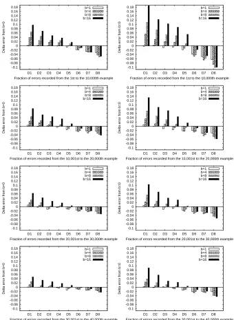
On the experimental side, we give evidence that our multitask algorithms provide a significant advantage over common baselines. In particular, we show that on a text categorization problem, where each task requires detecting the topic of a newsitem, a large multitask performance increase is attainable whenever the target topics are related. Additional experiments on a spam data set confirm the potential advantage of the p-norm Perceptron algorithm in a real-world setting.

This work is organized as follows. In Section 2 we introduce notation and formally define the adversarially chosen task protocol. The multitask Perceptron algorithm is presented in Section 3 where we also discuss the role of the multitask feature map and show (Section 4) that it can be used to turn online classifiers into multitask classifiers. We detail the matrix-based approach to the simultaneous multitask learning framework in Section 5. Section 6 is devoted to the theoretical analysis of a general potential-based algorithm for this setup. We conclude the paper with a number of experiments establishing the empirical effectiveness of our algorithms (Section 7).

1.2 Related Work

The problem of learning from multiple tasks has been the subject of a number of recently published papers. In Evgeniou et al. (2005) a batch multitask learning problem is defined as a regularized optimization problem and the notion of multitask kernel is introduced. More specifically, they con-sider a regularized functional that encodes multitask relations over tasks, thus biasing the solution of the problem towards functions that lie close to each other. Argyriou et al. (2007, 2008) build on this formalization to simultaneously learn a multitask classifier and the underlying spectral de-pendencies among tasks. A similar model but under cluster-based assumptions is investigated in Jacob et al. (2009). A different approach is discussed in Ando and Zhang (2005) where a structural risk minimization method is presented and multitask relations are established by enforcing predic-tive functions for the different tasks to belong to the same hypothesis set. Complexity results for multitask learning under statistical assumptions are also given in Maurer (2006).

Online linear multitask algorithms for the simultaneous task setting have been studied in Dekel et al. (2007), where the separate learning tasks are collectively dealt with through a common mul-titask loss. Their approach, however, is fundamentally different from the one considered here. In fact, using a common loss function has more the effect of prioritizing certain tasks over the others, whereas our regularized approach hopes to benefit from the information provided by each task to speed up the learning process for the other ones. Nonetheless, it is not difficult to extend our anal-ysis to consider a more sophisticated notion of multitask loss (see Remark 12 in Section 6.2), thus effectively obtaining a shared loss regularized multitask algorithm.

Online matrix approaches to the multitask and the related multiview learning problems were considered in various works. Matrix versions of the EG algorithm and the Winnow algorithm (re-lated to specific instances of the quasi-additive algorithms) have been proposed and analyzed in Tsuda et al. (2005), Warmuth (2007), and Warmuth and Kuzmin (2006). When dealing with the trace norm regularizer, their algorithms could be generalized to our simultaneous multitask frame-work to obtain mistake bounds comparable to ours. However, unlike those papers, we do not have learning rate tuning issues and, in addition, we directly handle general nonsquare task matrices.

Finally, Agarwal et al. (2008) consider multitask problems in the restricted expert setting, where task relatedness is enforced by a group norm regularization. Their results are essentially incompa-rable to ours.

2. The Adversarially Chosen Task Protocol: Preliminaries

The adversarially chosen task protocol works as follows. Let K be the number of binary

classifi-cation tasks indexed by 1, . . . ,K. Learning takes place in a sequential fashion: At each time step

t=1,2, . . .the learner receives a task index it∈ {1, . . . ,K}and observes an instance vector xt∈Rd which plays the role of side information for the task index it. Based on the pair xt,it

it outputs a binary predictiony_bt ∈ {−1,1}and then receives the correct label yt∈ {−1,1}for task index it. So, within this scheme, the learner works at each step on a single chosen task among the K tasks and operates under the assumption that instances from different tasks are vectors of the same dimension.

No assumptions are made on the mechanism generating the sequences x1,y1, x2,y2, . . . of task

examples. Moreover, similarly to Abernethy et al. (2007), the sequence of task indices i1,i2, . . . is also generated in an adversarial manner. To simplify notation we introduce a “compound” descrip-tion for the pair xt,it

and denote byφ_t∈RdKthe vector

φ⊤ t

def

= 0, . . . ,0 | {z } (it−1)d times

x_t⊤ 0, . . . ,0 | {z } (K₋it)d times

. (1)

Within this protocol (studied in Sections 3 and 4) we useφ_tor xt,itinterchangeably when referring

to a multitask instance. In the following we assume instance vectors are of (Euclidean) unit norm, that is,kxtk=1, so thatkφtk=1.

We measure the learner’s performance with respect to that of a (compound) reference predictor that is allowed to use a different linear classifier, chosen in hindsight, for each one of the K tasks. To remain consistent with the notation used for multitask instances, we introduce the “compound” reference task vector u⊤= u⊤₁, . . . ,u⊤_Kand define the hinge loss for the compound vector u as

ℓt(u) def

=max0,1₋ytu⊤φt =max

It is understood that the compound vectors are of dimension Kd. Our goal is then to compare the learner’s mistakes count to the cumulative hinge loss

∑

t

ℓt(u) (2)

suffered by the compound reference task vector u. This of course amounts to summing over time steps t the losses incurred by reference task vectors uit with respect to instance vectors xit.

In this respect, we aim at designing algorithms that make fewer mistakes than K independent learners when the tasks are related, and do not perform much worse than those when the tasks are completely unrelated. For instance, if we use Euclidean distance to measure task relatedness, we say that the K tasks are related if there exist reference task vectors u1, . . . ,uK ∈Rd having small pairwise distancesui−uj

, and achieving a small cumulative hinge loss in the sense of (2). More general notions of relatedness are investigated in the next sections.

Finally, we find it convenient at this point to introduce some matrix notation. We use Id to

refer to the d_×d identity matrix but drop the subscript whenever it is clear from context. Given

a matrix M_∈Rm×n we denote by Mi,j the entry that lies in the i-th row, j-th column. Moreover,

given two matrices M_∈Rm×nand N_∈Rm×rwe denote by[M,N]the m_×(n+r)matrix obtained

by the horizontal concatenation of M and N. The Kronecker or direct product between two matrices

M_∈Rm×nand N_∈Rq×ris the block matrix M_⊗N of dimension mq_×nr whose block on row i and

column j is the q_×r matrix Mi,jN.

3. The Multitask Perceptron Algorithm

We first introduce a simple multitask version of the Perceptron algorithm for the protocol described in the previous section. This algorithm keeps a weight vector for each task and updates all weight vectors at each mistake using the Perceptron rule with different learning rates. More precisely, let

wi,t be the weight vector associated with task i at time t. If we are forced (by the adversary) to

predict on task it, and our prediction happens to be wrong, we update wit,t−1through the standard

additive rule wit,t =wit,t−1+ηytxt (whereη>0 is a constant learning rate) but, at the same time, we perform a “half-update” on the remaining K₋1 Perceptrons, that is, we set wj,t=wj,t−1+η₂ytxt

for each j6=it. This rule is based on the simple observation that, in the presence of related tasks,

any update step that is good for one Perceptron should also be good for the others. Clearly, this rule keeps the weight vectors wj,t, j=1, . . . ,K, always close to each other.

The above algorithm is a special case of themultitask Perceptron algorithm described below.

This more general algorithm updates each weight vector wj,t through learning rates defined by a

K_×K interaction matrix A. It is A that encodes our beliefs about the learning tasks: different

choices of the interaction matrix result in different geometrical assumptions on the tasks.

The pseudocode for the multitask Perceptron algorithm using a generic interaction matrix A is given in Figure 1. At the beginning of each time step, the counter s stores the mistakes made

so far plus 1. The weights of the K Perceptrons are maintained in a compound vector w⊤_s =

w⊤_1,s, . . . ,w⊤_K,s, with wj,s∈Rd for all j. The algorithm predicts yt through the signybt of the it -th Perceptron’s margin w⊤_s−1φ_t =w⊤_it,s−1xt. Then, if the prediction and the true label disagree, the

compound vector update rule is ws=ws−1+ A⊗Id

−1_φ

t. Since A⊗Id −1

=A−1_⊗Id, the above update is equivalent to the K task updates

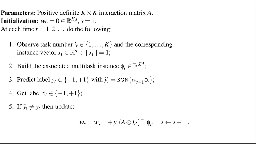
Parameters: Positive definite K_×K interaction matrix A. Initialization: w0=0∈RKd, s=1.

At each time t=1,2, . . . do the following:

1. Observe task number it∈ {1, . . . ,K}and the corresponding instance vector xt∈Rd : ||xt||=1;

2. Build the associated multitask instanceφ_{t ∈}RKd;

3. Predict label yt∈ {−1,+1}withybt=SGN w⊤_s−1φt

;

4. Get label yt ∈ {−1,+1};

5. Ify_bt 6=yt then update:

ws=ws−1+yt A⊗Id −1_φ

t, s←s+1.

Figure 1: The multitask Perceptron algorithm.

The algorithm is mistake-driven, hence ws−1 is updated (and s is increased) only whenbyt 6=yt. In

the following we use A_⊗ as a shorthand for A_⊗Id.

We now show that the algorithm in Figure 1 has the potential to make fewer mistakes than K independent learners when the tasks are related, and does not perform much worse than that when the tasks are completely unrelated. The bound dependence on the task relatedness is encoded as a quadratic form involving the compound reference task vector u and the interaction matrix A.

We specify the online multitask problem by the sequence(φ₁,y1),(φ₂,y2), . . ._∈RdK_{× {−1,1}} of multitask examples.

Theorem 1 The number of mistakes m made by the multitask Perceptron algorithm in Figure 1, run with an interaction matrix A on any finite multitask sequence of examples(φ₁,y1),(φ2,y2), . . .∈

RKd× {−1,1_}satisfies, for all u_∈RKd, m_≤

∑

t∈M

ℓt(u) + max i=1,...,K(A

−1₎

i,i u⊤A⊗u+ r

max i=1,...,K(A

−1₎

i,i u⊤A⊗u

∑

ℓt(u)

where

M

Theorem 1 is readily proven by using the fact that the multitask Perceptron is a specific instance of the kernel Perceptron algorithm, for example, Freund and Schapire (1999), using the so-called

linearmultitask kernel introduced in Evgeniou et al. (2005) (see also Herbster et al., 2005). This

kernel is defined as follows: for any positive definite K×K interaction matrix A introduce the

Kd-dimensional RKHS

H

feature mapψ:Rd× {1, . . . ,K_{} →}

H

K

=ψ(xs,is),ψ(xt,it)

Remark 2 Although the multitask kernel is appealing because it makes the definition of the mul-titask Perceptron simple and intuitive, one easily sees that the RKHS formalism is not neces-sary here since the kernel is actually linear. In fact, by re-defining the feature mapping as ψ:

Rd_{× {1, . . . ,K} →R}Kd_{, whereR}Kd_{is now endowed with the usual Euclidean product, and by} let-ting ψ(xt,it) =A−_⊗1/2φt, one gets an equivalent formulation of the multitask Perceptron based on A−_⊗1/2rather than A−_⊗1. In the rest of the paper we occasionally adopt this alternative linear kernel formulation, in particular whenever it makes the definition of the algorithm and its analysis simpler. Proof [Theorem 1] We use the following version of the kernel Perceptron bound (see, e.g., Cesa-Bianchi et al., 2005),

m_≤

∑

ℓt(h) +khk2H

max

t kψ(xt,it)k 2

H

+_kh_kHsmax

t kψ(xt,it)k 2

H

∑

t

ℓt(h)

where h is any function in the RKHS

H

observing that, for the kernel (3) we have

ku_k2_H =u⊤A_⊗u and _kψ(xt,it)k2H =φt⊤A−⊗1φt= (A−1)it,it

sinceφ_t singles out the it’s block of matrix A−_⊗1.

In the next three subsections we investigate the role of the quadratic form u⊤A_⊗u and specialize

Theorem 1 to different interaction matrices.

3.1 Pairwise Distance Interaction Matrix

The first choice of A we consider is the following simple update step (corresponding to the multitask Perceptron example we made at the beginning of this section).

wj,s=wj,s−1+ ( ₂

K+1ytxt if j=it, 1

K+1ytxt otherwise. As it can be easily verified, this choice is given by

A=

   

K ₋1 . . . ₋1

−1 K . . . ₋1

. . . .

−1 . . . K   

 (4)

with

A−1= 1

K+1    

2 1 . . . 1 1 2 . . . 1

. . . .

1 . . . 2     .

Corollary 3 The number of mistakes m made by the multitask Perceptron algorithm in Figure 1, run with the interaction matrix (4) on any finite multitask sequence of examples(φ₁,y1),(φ₂,y2), . . ._∈ RKd× {−1,1_}satisfies, for all u_∈RKd,

m≤

∑

t∈M

ℓt(u) +

2 u⊤A_⊗u K+1 +

v u u

t2 u⊤A⊗u K+1 _t

∑

∈M

ℓt(u)

where

u⊤A_⊗u=

K

∑

i=1

kuik2+

∑

1≤i<j≤K u_i−uj

2

.

In other words, running the Perceptron algorithm of Figure 1 with the interaction matrix (4) amounts to using the Euclidean distance to measure task relatedness. Alternatively, we can say that the

regularization term of the regularized target functional favors task vectors u1, . . . ,uK∈Rd having

small pairwise distancesui−uj

.

Note that when all tasks are equal, that is when u1=···=uK, the bound of Corollary 3 becomes

the standard Perceptron mistake bound (see, e.g., Cesa-Bianchi et al., 2005). In the general case of

distinct ui we have

2 u⊤A_⊗u K+1 =

2K K+1

K

∑

i=1

kuik2−

4

K+1_1≤i

∑

The sum of squares∑K_i=1kuik2 is the mistake bound one can prove when learning K independent

Perceptrons (under linear separability assumptions). On the other hand, highly correlated reference

task vectors (i.e., large inner products u⊤_i uj) imply a large negative second term in the right-hand

side of the above expression.

3.2 A More General Interaction Matrix

In this section we slightly generalize the analysis of the previous section and consider an update rule of the form

wj,s=wj,s₋1+

( b+K

(1+b)Kytxt if j=it, b

(1+b)Kytxt otherwise

where b is a nonnegative parameter. The corresponding interaction matrix is given by

A= 1

K    

a ₋b . . . ₋b

−b a . . . ₋b

. . . .

−b . . . a   

 (5)

with a=K+b(K₋1). It is immediate to see that the previous case (4) is recovered by choosing

b=K. The inverse of (5) is

A−1= 1 (1+b)K

   

b+K b . . . b b b+K . . . b

. . . .

When (5) is used in the multitask Perceptron algorithm, Theorem 1 can be specialized to the fol-lowing result.

Corollary 4 The number of mistakes m made by the multitask Perceptron algorithm in Figure 1, run with the interaction matrix (5) on any finite multitask sequence of examples(φ₁,y1),(φ2,y2), . . .∈

RKd× {−1,1_}satisfies, for all u_∈RKd,

m_≤

∑

ℓt(u) +

(b+K) (1+b)K u

⊤_A ⊗u+

s

(b+K)

(1+b)K u⊤A⊗u

∑

t∈M

ℓt(u)

where

u⊤A_⊗u=

K

∑

i=1

kuik2+bKVAR[u]

being VAR[u] = _K1∑K_i=1kui−uk2 the “variance”, of the task vectors, and u the centroid _K1 u1+

···+uK.

It is interesting to investigate how the above bound depends on the trade-off parameter b. The optimal value of b (requiring prior knowledge about the distribution of u1, . . . ,uK) is

b=max   0,

s

(K₋1) kuk

2 VAR[u]−1

   .

Thus b grows large as the reference task vectors ui get close to their centroid u (i.e., as all ui get

close to each other). Substituting this choice of b gives

(b+K) (1+b)K u

⊤_A ⊗u=

  

ku1_k2+_···+_kuKk2 if b=0,

kuk+√K−1pVAR[u]2 otherwise.

When the varianceVAR[u]is large (compared to the squared centroid normkuk2), then the optimal

tuning of b is zero and the interaction matrix becomes the identity matrix, which amounts to running K independent Perceptron algorithms. On the other hand, when the optimal tuning of b is nonzero

we learn K reference vectors, achieving a mistake bound equal to that of learning asingle vector

whose length is_ku_kplus√K₋1 times the standard deviationpVAR[u].

At the other extreme, if the variance VAR[u]is zero (namely, when all tasks coincide) then the

optimal b grows unbounded, and the quadratic term ₍(₁b₊+_bK_)K) u⊤A_⊗u tends to the average square norm _K1∑K_i=1kuik2. In this case the multitask algorithm becomes essentially equivalent to an al-gorithm that, before learning starts, chooses one task at random and keeps referring all instance

vectors xt to that task (somehow implementing the fact that now the information conveyed by it can

be disregarded).

3.3 Encoding Prior Knowledge

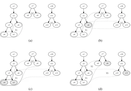
We could also pick the interaction matrix A so as to encode prior knowledge about tasks. For instance, suppose we know that only certain pairs of tasks are potentially related. We represent this

are connected by an edge if and only if we believe task i and task j are related. A natural choice for A is then A=I+L, where the K_×K matrix L is the Laplacian of G, defined as

Li,j=   

di if i= j,

−1 if(i,j)_∈E,

0 otherwise.

Here we denoted by dithe degree (number of incoming edges) of node i. If we now follow the proof

of Theorem 1, which holds for any positive definite matrix A, we obtain the following result.

Corollary 5 The number of mistakes m made by the multitask Perceptron algorithm in Figure 1, run with the interaction matrix I+L on any finite multitask sequence of examples(φ₁,y1),(φ2,y2), . . .∈

RKd_{× {−1,1}satisfies, for all u∈R}Kd_, m_≤

∑

t∈M

ℓt(u) +cGu⊤ I+L

⊗u+ r

cGu⊤ I+L

⊗u

∑

ℓt(u)

where

u⊤ I+L ⊗u=

K

∑

i=1

kuik2+

∑

(i,j)∈E u_i−uj

2

(6)

and cG=maxi=1,...,K∑Kj=1 v2

j,i

1+λj. Here 0=λ1<λ2≤ ··· ≤λK are the eigenvalues of the positive semidefinite matrix L, and vj,idenotes the i-th component1of the eigenvector vjof L associated with eigenvalueλj.

Proof Following the proof of Theorem 1, we just need to bound

max i=1,...,KA

−1

i,i =_i=max_1,...,K(I+L)− 1 i,i .

If v1, . . . ,vKare the eigenvectors of L, then

(I+L)−1=

K

∑

j=1 vjv⊤j 1+λj

which concludes the proof.

Ideally, we would like to have cG=O _K1

. Clearly enough, if G is the clique on K vertices we expect to exactly recover the bound of Theorem 1. In fact, we can easily verify that the eigenvector v1 associated with the zero eigenvalueλ1 is K−1/2, . . . ,K−1/2

. Moreover, it is well known that

all the remaining eigenvalues are equal to K—see, for example, Hogben (2006). Therefore cG=

1

K+ 1− 1 K

1 K+1 =

2

K+1. In the case of more general graphs G, we can bound cGin terms of the

smallest nonzero eigenvalueλ2,

cG≤ 1 K+

1₋ 1

K

1

1+λ2 .

The value ofλ2, known as the algebraic connectivity of G, is 0 only when the graph is disconnected.

λ2is known for certain families of graphs. For instance, if G is a complete bipartite graph (i.e., if

tasks can be divided in two disjoint subsets T1and T2such that every task in T1is related to every task in T2and for both i=1,2 no two tasks in Ti are related), then it is known thatλ2=min|T1|,|T2| . The advantage of using a graph G with significantly fewer edges than the clique is that the sum

of pairwise distances in (6) will contain less than K₂terms. On the other hand, this reduction has

to be contrasted to a larger coefficient cGin front of u⊤ I+L_⊗u. This coefficient, in general, is

related to the total number of edges in the graph (observe that the trace of L is exactly twice this total number). The role of prior knowledge is thus to avoid the insertion in A of edges connecting

tasks that are hardly related, thus preventing the presence of large terms in the sum u⊤ I+L_⊗u.

4. Turning Perceptron-like Algorithms Into Multitask Classifiers

We now show how to obtain multitask versions of well-known classifiers by using the multitask kernel mapping detailed in Section 3.

4.1 The Multitask p-norm Perceptron Algorithm

We first consider the p-norm Perceptron algorithm of Grove et al. (2001) and Gentile (2003). As before, when the tasks are all equal we want to recover the bound of the single-task algorithm, and when the task vectors are different we want the mistake bound to increase according to a function that penalizes task diversity according to their p-norm distance.

The algorithm resembles the Perceptron algorithm and maintains its state in the compound

pri-mal weight vector vs∈RKd where s stores the mistakes made so for (plus one). What sets the

multitask p-norm Perceptron aside from the algorithm of Section 3 is that the prediction at time t is computed, for an arbitrary positive definite interaction matrix A, as SGN w⊤_s−1A−_⊗1φ_t where

thedual weight vector ws−1is a (one-to-one) transformation of the weight vector vs−1, specifically

ws₋1=∇1₂kvs₋1k2_p, with p≥2. If a mistake occurs at time t, vs₋1∈RKd is updated using the multitask Perceptron rule, vs=vs−1+ytA−_⊗1φt . We are now ready to state the mistake bound for the the multitask p-norm Perceptron algorithm. In this respect we focus on a specific choices of p and A.

Theorem 6 The number of mistakes m made by the p-norm multitask Perceptron, run with the pairwise distance matrix (4) and p=2 ln max_{K,d_}, on any finite multitask sequence of examples

(φ₁,y1),(φ2,y2), . . .∈RKd× {−1,1}satisfies, for all u∈RKd, m≤

∑

t∈M

ℓt(u) +H+ r

2H

∑

t∈M

ℓt(u)

where

H=8 e

2_{ln max{K,d}}

(K+1)2 X 2

∞

K

∑

i=1 ui+

∑

j6=i

ui−uj 1

!2

and X_∞=max_t∈M kxtk_∞.

Proof Let vmbe the primal weight vector after any number m of mistakes. By Taylor-expanding 1

2kvsk 2

paround vs−1for each s=1, . . . ,m, and using the fact ytw⊤s−1A− 1

⊗ φt ≤0 whenever a mistake

occurs at step t, we get

1 2kvmk

2 p≤

m

∑

s=1

where D(vskvs₋1) =1₂

kvsk2_p− kvs₋1k2_p

−ytw⊤_s−1A−_⊗1φt is the so-called Bregman divergence, that is, the error term in the first-order Taylor expansion of 1_2k·k2_paround vector vs−1, at vector vs.

Fix any u∈RKd. Using the convex inequality for norms u⊤v≤ kukqkvkpwhere q=p/(p−1) is the dual coefficient of p (so that_k·kqis the dual norm of_k·kp), and the fact that

u⊤A_⊗vs=u⊤A_⊗vs₋1+ytu⊤φt ≥u⊤A⊗vs₋1+1−ℓt(u), one then obtains

kvmkp≥

u⊤A_⊗vm

kA_⊗u_kq ≥

m₋∑_t∈Mℓt(u)

kA_⊗u_kq . (8)

Combining (7) with (8) and solving for m gives

m_≤

∑

ℓt(u) +kA_⊗uk_q s

2 m

∑

s=1

D(vskvs₋1). (9) Following the analysis contained in, for example, Cesa-Bianchi and Lugosi (2006), one can show

that the Bregman term can be bounded as follows, for ts=t,

D(vskvs₋1)≤ p₋1

2 A−1

⊗ φt 2

p= p₋1

2 kxtk 2 p A−_↓i1

t 2_p where A−_↓i1

t is the it-th column of A −1_.

We now focus our analysis on the choice p=2 ln max_{K,d_} which gives mistake bounds in

the dual norms_ku_k1 and_kxtk_∞, and on the pairwise distance matrix (4). It is well known that for

p=2 ln d the mistake bound of the single-task p-norm Perceptron is essentially equivalent to the

one of the zero-threshold Winnow algorithm of Littlestone (1989). We now see that this property is preserved in the multitask extension. We have_kxtk2p≤ekxtk2_∞and

A−_↓i1

t 2_p≤e

A−_↓i1

t

2_∞=e A−_it,1_it2= 4 e (K+1)2 . As for the dual norm_kA_⊗u_kq, we get

kA_⊗u_k2_{q≤ k}A_⊗u_k2₁=

K

∑

i=1 ui+

∑

j6=i

ui−uj 1

!2

.

Substituting into (9) gives the desired result.

The rightmost factor in the expression for H in the statement of Theorem 6 reveals the way similarity

among tasks is quantified in this case. To gain some intuition, assume the task vectors ui are all

sparse (few nonzero coefficients). Then H is small when the task vectors ui have a common pattern

of sparsity; that is, when the nonzero coordinates tend to be the same for each task vector. In the extreme case when all task vectors are equal (and not necessarily sparse), H becomes

K K+1

2

8 e2ln max_{K,d_} max t=1,...,nkxtk∞

2

ku1k21 . (10)

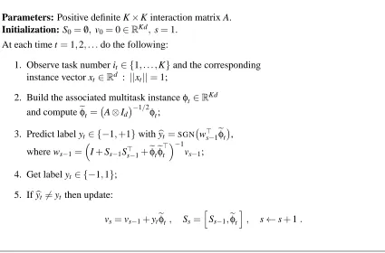
Parameters: Positive definite K_×K interaction matrix A. Initialization: S0=/0, v0=0∈RKd,s=1.

At each time t=1,2, . . .do the following:

1. Observe task number it∈ {1, . . . ,K}and the corresponding instance vector xt∈Rd : ||xt||=1;

2. Build the associated multitask instanceφ_{t ∈}RKd

and computeeφ_t= A_⊗Id

−1/2_φ t;

3. Predict label yt∈ {−1,+1}withbyt=SGN w⊤s₋1eφt

,

where ws−1=

I+Ss−1Ss⊤−1+eφteφ ⊤ t

−1 vs−1; 4. Get label yt ∈ {−1,1};

5. Ify_bt 6=yt then update:

vs=vs−1+yteφt , Ss= h

Ss−1,eφt i

, s_←s+1.

Figure 2: The second-order multitask Perceptron algorithm.

Remark 7 Note that for p=2 our p-norm variant of the multitask Perceptron algorithm does not reduce to the multitask Perceptron of Figure 1. In order to obtain the latter as a special case of the former, we could use the fact that the multitask Perceptron algorithm is equivalent to the standard

2-norm Perceptron run on “multitask instances” A−_⊗1/2φ_t—see Remark 2. One then obtains a proper

p-norm generalization of the multitask Perceptron algorithm by running the standard p-norm Per-ceptron on such multitask instances. Unfortunately, this alternative route apparently prevents us from obtaining a bound as good as the one proven in Theorem 6. For example, when p is chosen as in Theorem 6 and all task vectors are equal, then multitask instances of the form A−_⊗1/2φ_t yield a bound K times worse than (10), which is obtained with instances of the form A−_⊗1φ_t.

Finally, we should mention that an alternative definition of the p-norm Perceptron for a related problem of predicting a labelled graph has been recently proposed in Herbster and Lever (2009).

4.2 The Multitask Second-order Perceptron Algorithm

We now turn to the second-order kernel Perceptron algorithm of Cesa-Bianchi et al. (2005). The algorithm, described in Figure 2, maintains in its internal state a matrix S (initialized to the empty

matrix /0) and a multitask Perceptron weight vector v (initialized to the zero vector). Just like in

Figure 1, we use the subscript s to denote the current number of mistakes plus one. The algorithm computes a tentative (inverse) matrix

I+Ss−1S⊤s−1+eφteφ ⊤ t

−1

Such a matrix is combined with the current Perceptron vector vs−1to predict the label yt. If the pre-diction_bytand the label ytdisagree both vs₋1and Ss₋1get updated (no update takes place otherwise).

In particular, the new matrix Ssis augmented by padding with the current vectoreφt. Since supports

are shared, the computational cost of an update is not significantly larger than that for learning a single-task (see Subsection 4.2.1).

Theorem 8 The number of mistakes m made by the multitask Second Order Perceptron algo-rithm in Figure 2, run with an interaction matrix A on any finite multitask sequence of examples

(φ₁,y1),(φ₂,y2), . . ._∈RKd× {−1,1_}satisfies, for all u_∈RKd,

m_≤

∑

ℓt(u) + v u u

t _u⊤_A⊗u+

∑

u⊤_itxt2 ! _m

∑

j=1

ln(1+λj)

where

M

M

Proof From the mistake bound for the kernel second-order Perceptron algorithm (Cesa-Bianchi et al., 2005) we have, for all h in

H

m_≤

∑

ℓt(h) + v u u t _khk2

H +

∑

t∈M

h(φ_t)2 ! _m

∑

i=1

ln(1+λi)

where λ1, . . . ,λm are the eigenvalues of the kernel Gram matrix including only time steps in

M

Making the role of A_⊗explicit in the previous expression yields

kuk2H =u⊤A⊗u

and

u,ψ(xt,it)2_H =

u⊤A_⊗A−_⊗1φ_t2=u⊤_itxt 2

.

Finally, the kernel Gram matrix has elements

K

=φ⊤_sA−_⊗1φ_t =x⊤_sA−_i 1

s,itxt, where

s,t_∈

M

Again, this bound should be compared to the one obtained when learning K independent tasks.

As in the Perceptron algorithm, we have the complexity term u⊤A_⊗u. In this case, however, the

interaction matrix A also plays a role in the scale of the eigenvalues of the resulting multitask Gram matrix. Roughly speaking, when the tasks are close and A is the pairwise distance matrix, we essentially gain a factor√K from the fact that u⊤A_⊗u is close to K times the complexity of the single task (according to the arguments in Section 3). On the other hand, the trace of the multitask Gram matrixφ⊤_sA−_⊗1φ_ts,t

∈M = [x⊤sA−is,1itxt

s,t∈M is about the same as the trace of the single task matrix,

since the K times larger dimension of the multitask matrix is offset by the factor 1/K delivered

by A−_⊗1 in φ⊤_sA−_⊗1φ_ts,t

∈M when compared to the single task Gram matrix

x⊤_sxt

s,t_∈M. So, in a

sense, the spectral quantity∑m_j=1ln(1+λj) is similar to the corresponding quantity for the single task case. Putting together, unlike the first-order Perceptron, the gain factor achieved by a multitask

4.2.1 IMPLEMENTINGTHEMULTITASKSECOND-ORDERPERCEPTRONINDUALFORM

It is easy to see that the second-order multitask Perceptron can be run in dual form by maintaining K classifiers that share the same set of support vectors. This allows an efficient implementation that does not impose any significant overhead with respect to the corresponding single-task version.

Specifically, given some interaction matrix A the margin at time t is computed as (see Cesa-Bianchi et al., 2005, Theorem 3.3)

w⊤_s−1eφ_t =v⊤_s−1I+Ss−1S⊤s₋1+eφteφ ⊤ t

−1 eφ_t

=y⊤_sI+S⊤_sSs −1

S_s⊤eφ_t (11)

where y_sis the s-dimensional vector whose first s₋1 components are the labels yi where the

algo-rithm has made a mistake up to time t₋1, and the last component is 0.

Note that replacing I+S⊤_sSswith I+S⊤s−1Ss−1in (11) does not change the sign of the

predic-tion. The margin at time t can then be computed by calculating the scalar product between S⊤_seφ_t

and y⊤_s I+S⊤_s−1Ss−1 −1

. Now, each entry of the vector S_s⊤eφ_t is of the form A−_j,i1 tx

⊤

jxt, and thus com-puting S⊤_seφ_t requires O(s) inner products so that, overall, the prediction step requires O(s) scalar

multiplications and O(s)inner products (independent of the number of tasks K).

On the other hand, the update step involves the computation of the vector y⊤_s I+S_s⊤Ss−

1 . For the matrix update we can write

I+S⊤_sSs= "

I+S⊤_s−1Ss−1 S⊤s−1eφt e

φ⊤t Ss₋1 1+eφ⊤t eφt #

.

Using standard facts about the inverse of partitioned matrices (see, e.g., Horn and Johnson, 1985,

Ch. 0), one can see that the inverse of matrix I+S⊤_sSs can be computed from the inverse of

I+S⊤_s−1Ss−1 with O(s)extra inner products (again, independent of K) and O(s2) additional scalar multiplications.

5. The Simultaneous Multitask Protocol: Preliminaries

The multitask kernel-based regularization approach adopted in the previous sections is not the only way to design algorithms for the multiple tasks scenario. As a different strategy, we now aim at mea-suring tasks relatedness as a function of the dimension of the space spanned by the task reference vectors. In matrix terms, this may be rephrased by saying that we hope to speed up the learning pro-cess, or reduce the number of mistakes, whenever the matrix of reference vectors is spectrally sparse. For reasons that will be clear in a moment, and in order to make the above a valid and reasonable goal for a multitask algorithm, we now investigate the problem of simultaneously producing multiple predictions after observing the corresponding (multiple) instance vectors. We therefore extend the traditional online classification protocol to a fully simultaneous multitask environment where at each time step t the learner observes exactly K instance vectors xi,t ∈Rd,i=1, . . . ,K. The learner then outputs K predictions_byi,t∈ {−1,+1}and obtains the associated labels yi,t∈ {−1,+1},i=1, . . . ,K.

We still assume that the K example sequences are adversarially generated and that_kxi,tk=1. We

Once again the underlying rationale here is that one should be able to improve the performance over the baseline by leveraging the additional information conveyed through multiple instance vec-tors made available all at once, provided that the tasks to learn share common characteristics. Theo-retically, this amounts to postulating the existence of K vectors u1, . . . ,uKsuch thateach uiis a good linear classifier for the corresponding sequence(xi,1,yi,1),(xi,2,yi,2), . . .of examples. As before, the natural baseline is the algorithm that simultaneously run K independent Perceptron algorithms, each one observing its own sequence of examples and acting in a way that is oblivious to the instances given as input to and the labels observed by its peers. Of course, we now assume that this baseline outputs K predictions per trial. The expected performance of this algorithm is simply K times the one of a single Perceptron algorithm. An additional difference that sets the protocol and the algo-rithms discussed here apart from the ones considered in the previous sections is that the cumulative count of mistakes is not only over time but also over tasks; that is, at each time step more the one

mistake might occur since K>1 predictions are output.

In the next section we show that simultaneous multitask learning algorithms can be designed in such a way that the cumulative number of mistakes is, in certain relevant cases, provably better than the K independent Perceptron algorithm. The cases where our algorithms outperform the latter are exactly those when the overall information provided by the different example sequences are related, that is, when the reference vectors associated with different tasks are “similar”, while the instance vectors received during each time step are unrelated (and thus overall more informative). These notions of similarity and unrelatedness among reference and instance vectors will be formally defined later on.

5.1 Notation and Definitions

We denote by _hM,N_i=TR M⊤N, for M,N ∈Rd×K the Frobenious matrix inner product. Let

r=min_{d,K_}and define the functionσ:Rd×K→Rrsuch thatσ(M) = σ1(M), . . . ,σr(M)

, where

σ1(M)_{≥ ··· ≥}σr(M)≥0 are the singular values of a matrix M∈Rd×K. In the following, we simply

writeσiinstead ofσi(M)whenever the matrix argument is clear from the context.

Following Horn and Johnson (1991) we say that a function f :Rr→Ris a symmetric gauge

function if it is an absolute norm onRr and is invariant under permutation of the components of

its argument. We consider matrix norms of the form_k·k:Rd×K →Rsuch that_k·k= f_◦σwhere

f is symmetric gauge function. A matrix norm is said unitarily (orthogonally, indeed, since we

only consider matrices with real entries) invariant if_kUAV_k=_kA_kfor any matrix A and for any

unitary (orthogonal) matrices U and V for which UAV is defined. It is well known that a matrix norm is unitarily invariant if and only if it is a symmetric gauge function of the singular values of its argument.

One important class of unitarily invariant norms is given by the Schatten p-norms, kUksp

def

=

kσ(U)_kp, where the right-hand expression involves a vector norm. Note that the Schatten 2-norm is

the Frobenius norm, while for p=1 the Schatten p-norm becomes the trace norm_kU_ks1=_kσ(U)_k1,

which is a good proxy for the rank of U ,_kσ(U)_k0.

Let M be a matrix of size d_×K. We denote by VEC(M) the vector of size Kd obtained by

stacking the columns of M one underneath the other. Important relationships can be established

among the Kronecker product, theVECoperator and the trace operator. In particular, we have

for any M,N,O for which MNO is defined, and

VEC(M)⊤VEC(N) = TR(M⊤N) (13)

for any M,N of the same order. We denote by TK2 the K2×K2 commutation matrix such that

T_K2VEC(M) =VEC(M⊤). We recall that T_K2also satisfies T_K2(M⊗N) = (M⊗N)T_K2for any M,N∈

Rd×K.

We rely on the notation introduced by Magnus and Neudecker (1999) to derive calculus rules

for functions defined over matrices. Given a differentiable function F :Rm×p→Rn×q, we define

the Jacobian of F at M as the matrix∇F(M)_∈Rnq×mp

∇F(X) =∂VEC F(M)

∂VEC(M)⊤ . (14) It is easy to see that (14) generalizes the well-known definition of Jacobian for vector valued

func-tions of vector variables. The following rules, which hold for any matrix M_∈RK×K, can be seen as

extensions of standard vector derivation formulas

∇TR(Mp) = pVEC(Mp−1)⊤ p=1,2, . . . (15) ∇M⊤_{M = (I}

K2+T_K2)(I_K⊗M⊤). (16)

6. The Potential-based Simultaneous Multitask Classifier

As discussed in Section 5, a reasonable way to quantify the similarity among reference vectors, as well as the unrelatedness among example vectors, is to arrange such vectors into matrices, and then deal with special properties of these matrices. In order to focus on this concept, we lay out vectors

as columns of d_×K matrices and extend the dual norm analysis of Subsection 4.1 to matrices. The

idea is to design a classifier which is able to perform much better than the K independent Perceptron

baseline discussed in Section 5 whenever the set of reference vectors ui∈Rd (arranged into a d×K

reference matrix U ), have some matrix-specific, for example, spectral, properties.

Our potential-based matrix algorithm for classification shown in Figure 3 generalizes the classi-cal potential-based algorithms operating on vectors to simultaneous multitask problems with matrix examples. This family of potential-based algorithms has been introduced in the learning literature by Kivinen and Warmuth (2001) and Grove et al. (2001), and by Nemirovski and Yudin (1978) and Beck and Teboulle (2003) in the context of nonsmooth optimization. The algorithm maintains a d×K matrix W . Initially, W0 is the zero matrix. If s−1 updates have been made in the first t₋1 time steps, then the K predictions at time t areSGN w⊤_i,s−1xi,t, i=1, . . . ,K, where the vector wi,s−1∈Rd is the i-th column of the the d×K matrix Wsand xi,t ∈Rd is the instance vector asso-ciated with the i-th task at time t. An update is performed if at least one mistake occurs. When the s-th update occurs at time t then Wsis computed as

Ws=∇ 1 2kVsk

2

where, in turn, the columns of the d×K matrix Vsare updated using the Perceptron rule,2 vi,s=

vi,s₋1+yi,txi,t1

{byi,t6=yi,t} which, as in the basic Perceptron algorithm, is mistake driven. In other 2. Here and throughout this section,1

{byi,t6=yi,t}denotes the indicator function which is 1 if the label associated with the

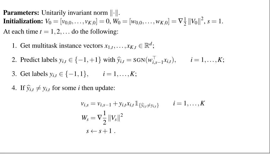
Parameters: Unitarily invariant norm_k·k.

Initialization: V0= [v0,0, . . . ,vK,0] =0, W0= [w0,0, . . . ,wK,0] =∇1₂kV0k2, s=1. At each time t=1,2, . . .do the following:

1. Get multitask instance vectors x1,t, . . . ,xK,t∈Rd;

2. Predict labels yi,t∈ {−1,+1}withbyi,t =SGN(w⊤_i,s−1xi,t), i=1, . . . ,K; 3. Get labels yi,t ∈ {−1,1}, i=1, . . . ,K;

4. Ify_bi,t 6=yi,t for some i then update:

vi,s=vi,s−1+yi,txi,t1

{byi,t6=yi,t} i=1, . . . ,K Ws=∇

1 2kVsk

2 s_←s+1.

Figure 3: The potential-based matrix algorithm for the simultaneous multitask setting.

words, the i-th column in Vs₋1 is updated if and only if the label associated with the i-th task was

wrongly predicted. We say that Ws is the dual matrix weight associated with the primal matrix

weight Vs. So far we left the mapping from Vs to Ws partially unspecified since we did not say

anything other than it is the gradient of some unitarily invariant (squared) norm.

6.1 Analysis of Potential-based Matrix Classifiers

We now develop a general analysis of potential-based matrix algorithms for (simultaneous) multi-task classification. Then, in Section 6.2 we specialize it to Schatten p-norms. The analysis proceeds along the lines of the standard proof for potential-based algorithms. Before turning to the details,

we introduce a few shorthands. Let1i,t=1

{ybi,t6=yi,t}, and1t be the K-dimensional vector whose i-th

component is1i,t. Also, ei denotes the i-th vector of the standard basis forR

K_{. Finally, we define}

the matrix Mt=∑Ki=11i,tyi,txi,te

⊤

i whose i-th column is the example vector yi,txi,t if the label yi,t was wrongly predicted at time t, or the null vector otherwise. It is easy to see that, by using this notation, the update of the primal weight matrix V can be written as Vs=Vs−1+Mt.

Let

M

m=_|

M

1 2kVmk

2

≤

m

∑

s=1

where D(VskVs−1) =1₂ kVsk2−kVs−1k2

−hWs−1,Mtiis the matrix Bregman divergence associated

with∇1_2k·k2. The upper bound in (17) follows from

hWs−1,Mti=TR(Ws⊤₋1Mt) =

K

∑

i=1

1i,tyi,tw

⊤

s₋1xi,t≤0

the last inequality holding because1i,t is 1 if only if a mistake in the prediction for the i-th task

occurs at time t.

Fix any d_×K comparison matrix U and denote by _k·k∗the matrix dual norm. By the convex

inequality for matrix norms we have_kVmkkUk_∗≥ hVm,Ui, wherekUk_∗= f∗ σ(U)and f∗is the Legendre dual of function f —see Lewis (1995, Theorem 2.4). From_hU,Vsi=hU,Vs−1i+hU,Mti. we obtain

kVmk ≥h

U,Vmi

kU_k∗ ≥

∑t∈M k1tk

1−∑t∈Mℓ1

t(U)

kU_k∗

where

ℓ1

t (U) def

=

K

∑

i=1

1i,t

1−yi,tu⊤i xi,t

+=

K

∑

i=1

1i,tℓt(ui)

and_k1tk

1counts the number of mistaken tasks at time t. Solving for µ=∑t∈Mk1tk

1gives

µ_≤

∑

ℓ1

t(U) +kUk_∗ s

2 m

∑

s=1

D(VskVs₋1). (18)

Equation (18) is our general starting point for analyzing potential-based matrix multitask algorithms. In particular, the analysis reduces to bounding from above the Bregman term for the specific matrix norm under consideration.

6.2 Specialization to Schatten p-norms

In this section we focus on Schatten p-norms, therefore measuring similarity (or dissimilarity) in terms of spectral properties. This amounts to saying that a set of reference vectors are similar if they span a low dimensional subspace. Along the same lines, we say that a set of K example vectors are dissimilar if their spanned subspace has dimension close to K. The rank of a matrix whose columns are either the reference vectors or the example vectors exactly provides this information. Here we use certain functions of the singular values of a matrix as proxies for its rank. It is easy to see that this leads to a kind of regularization that is precisely enforced through the use of unitarily-invariant norms. In fact, unitarily-invariant matrix norms control the distribution of the singular values of U , thus acting as spectral co-regularizers for the reference vectors—see, for example, Argyriou et al. (2008) for recent developments on this subject. In different terms, by relying only on the singular values (or on the magnitudes of principal components), unitarily invariant norms are a natural way to determine and measure the most informative directions for a given set of vectors.

For these reasons we now specialize the potential-based matrix classifier of Figure 3 to the

Schatten 2p-norm and set_kV_k=_kV_ks

2p=kσ(V)k2p,where V is a generic d×K matrix, and p is a

positive integer (thus 2p is an even number_≥2). Note that, in general,

kV_k2_s

2p=TR (V

⊤_V)p1/p

We are now ready to state our main result of this section. The proof, along with surrounding comments, can be found in the appendix.

Theorem 9 The overall number of mistakes µ made by the 2p-norm matrix multitask Perceptron (with p positive integer) run on finite sequences of examples (xi,1,y1,t),(xi,2, ,yi,2),··· ∈Rd×K×

{−1,+1_}, for i=1, . . . ,K, satisfies, for all U_∈Rd×K,

µ_≤

∑

ℓ1

t (U) + (2p−1)

Ms2pkUks2q

2

+Ms2pkUks2q

r

(2p₋1)

∑

t_∈M

ℓ1

t (U)

where

Ms2p=max

t∈M

kMtks2p

p

k1tk

1 and_kU_ks

2q is the Schatten 2q-norm of U , with 2q=

2p 2p−1.

Remark 10 In order to verify that in certain cases the bound of Theorem 9 provides a significant improvement over the K independent Perceptron baseline, we focus on the linearly separable case; that is, when the sequences(xi,1,yi,1),(xi,2,yi,2), . . . are such that there exists a matrix U ∈Rd×K whose columns ui achieve a margin of at least 1 on each example: yi,tu⊤i xi,t≥1 for all t=1,2, . . . and for all i=1, . . . ,K. In this case the bound of Theorem 9 reduces to

µ_≤(2p₋1)Ms2pkUks2q

2

. (19)

It is easy to see that for p=q=1 the 2p-norm matrix multitask Perceptron decomposes into K independent Perceptrons, which is our baseline. On the other hand, similarly to the vector case, a trace norm/spectral norm bound can be established when the parameter p is properly chosen. Note first that for basic properties of norms_kU_ks

2q ≤ kUks1 andkMks2p≤r

1/(2p)_kMk

s∞, with r=

min_{d,K_}. It now suffices to set p=_⌈ln r_⌉in order to rewrite (19) as µ_≤(2 ln r+1)e Ms∞kUks1

2

where U is now penalized with the trace norm and Mt is measured with the spectral normk·ks∞. If

the columns of U span a subspace of dimension_≪K, and the matrices of mistaken examples Mt tend to have K nonzero singular values of roughly the same magnitude, then_kU_ks

1 ≈ kUks2 while

M2_s∞≈M2_s2/K. Hence this choice of p may lead to a factor K improvement over the bound achieved by the independent Perceptron baseline. See also Remark 11 below. Note that in Theorem 9 (and in the above argument) what matters the most is the quantification in terms of the spectral properties of U via _kU_ks

2q. The fact that p has to be a positive integer is not a big limitation here, since

2q=_2p2p₋₁ can be made arbitrarily close to 1 anyway.

Remark 11 The bound of Theorem 9 is not in closed form, since the terms_k1tk

1occur in both the left-hand side (via µ) and in the right-hand side (via Ms2p). These terms play an essential role to

assess the potential advantage of the 2p-norm matrix multitask Perceptron. In order to illustrate the influence of_k1tk

1on the bound, let us consider the two extreme casesk1tk

1=1 for all t∈

M

k1tk