Spectral Regularization Algorithms for Learning Large Incomplete Matrices

Spectral Regularization Algorithms for Learning Large Incomplete

Matrices

Rahul Mazumder [email protected]

Trevor Hastie∗ [email protected]

Department of Statistics Stanford University Stanford, CA 94305

Robert Tibshirani† [email protected]

Department of Health, Research and Policy Stanford University

Stanford, CA 94305

Editor: Tommi Jaakkola

Abstract

We use convex relaxation techniques to provide a sequence of regularized low-rank solutions for large-scale matrix completion problems. Using the nuclear norm as a regularizer, we provide a sim-ple and very efficient convex algorithm for minimizing the reconstruction error subject to a bound on the nuclear norm. Our algorithm SOFT-IMPUTEiteratively replaces the missing elements with those obtained from a soft-thresholded SVD. With warm starts this allows us to efficiently compute an entire regularization path of solutions on a grid of values of the regularization parameter. The computationally intensive part of our algorithm is in computing a low-rank SVD of a dense matrix. Exploiting the problem structure, we show that the task can be performed with a complexity of or-der linear in the matrix dimensions. Our semidefinite-programming algorithm is readily scalable to large matrices; for example SOFT-IMPUTEtakes a few hours to compute low-rank approximations of a 106_×106_{incomplete matrix with 10}7_{observed entries, and fits a rank-95 approximation to the}

full Netflix training set in 3.3 hours. Our methods achieve good training and test errors and exhibit superior timings when compared to other competitive state-of-the-art techniques.

Keywords: collaborative filtering, nuclear norm, spectral regularization, netflix prize, large scale

convex optimization

1. Introduction

In many applications measured data can be represented in a matrix Xm×n,for which only a

rela-tively small number of entries are observed. The problem is to “complete” the matrix based on the observed entries, and has been dubbed the matrix completion problem (Cand`es and Recht, 2008; Cand`es and Tao, 2009; Rennie and Srebro, 2005). The “Netflix” competition (for example, SIGKDD and Netflix, 2007) is a popular example, where the data is the basis for a recommender system. The rows correspond to viewers and the columns to movies, with the entry Xi j being the

rating∈ {1, . . . ,5}by viewer i for movie j. There are about 480K viewers and 18K movies, and hence 8.6 billion (8.6×109) potential entries. However, on average each viewer rates about 200

movies, so only 1.2% or 108 entries are observed. The task is to predict the ratings that viewers would give to movies they have not yet rated.

These problems can be phrased as learning an unknown parameter (a matrix Zm×n) with very

high dimensionality, based on very few observations. In order for such inference to be meaningful, we assume that the parameter Z lies in a much lower dimensional manifold. In this paper, as is relevant in many real life applications, we assume that Z can be well represented by a matrix of low rank, that is, Z≈Vm×kGk×n, where k≪min(n,m). In this recommender-system example, low rank

structure suggests that movies can be grouped into a small number of “genres”, with Gℓjthe relative

score for movie j in genreℓ. Viewer i on the other hand has an affinity Viℓfor genreℓ, and hence the

modeled score for viewer i on movie j is the sum∑k_ℓ=1ViℓGℓjof genre affinities times genre scores.

Typically we view the observed entries in X as the corresponding entries from Z contaminated with noise.

Srebro et al. (2005a) studied generalization error bounds for learning low-rank matrices. Re-cently Cand`es and Recht (2008), Cand`es and Tao (2009), and Keshavan et al. (2009) showed the-oretically that under certain assumptions on the entries of the matrix, locations, and proportion of unobserved entries, the true underlying matrix can be recovered within very high accuracy.

For a matrix Xm×nlet Ω⊂ {1, . . . ,m} × {1, . . . ,n}denote the indices of observed entries. We

consider the following optimization problem:

minimize rank(Z)

subject to

∑

(Xi j−Zi j)2≤δ, (1)

whereδ≥0 is a regularization parameter controlling the tolerance in training error. The rank con-straint in (1) makes the problem for generalΩcombinatorially hard (Srebro and Jaakkola, 2003). For a fully-observed X on the other hand, the solution is given by a truncated singular value decom-position (SVD) of X . The following seemingly small modification to (1),

minimize kZk∗

subject to

∑

(Xi j−Zi j)2≤δ, (2)

makes the problem convex (Fazel, 2002). HerekZk∗is the nuclear norm, or the sum of the singular

values of Z. Under many situations the nuclear norm is an effective convex relaxation to the rank constraint (Fazel, 2002; Cand`es and Recht, 2008; Cand`es and Tao, 2009; Recht et al., 2007). Op-timization of (2) is a semi-definite programming problem (Boyd and Vandenberghe, 2004) and can be solved efficiently for small problems, using modern convex optimization software like SeDuMi and SDPT3 (Grant and Boyd., 2009). However, since these algorithms are based on second order methods (Liu and Vandenberghe, 2009), they can become prohibitively expensive if the dimensions of the matrix get large (Cai et al., 2008). Equivalently we can reformulate (2) in Lagrange form

minimize

Z

1

2_(i,

∑

2_+λkZk

∗. (3)

In this paper we propose an algorithm SOFT-IMPUTE for the nuclear norm regularized least-squares problem (3) that scales to large problems with m,n≈105–106with around 106–108or more observed entries. At every iteration SOFT-IMPUTEdecreases the value of the objective function towards its minimum, and at the same time gets closer to the set of optimal solutions of the prob-lem (2). We study the convergence properties of this algorithm and discuss how it can be extended to other more sophisticated forms of spectral regularization.

To summarize some performance results1

• We obtain a rank-40 solution to (2) for a problem of size 105×105_and|Ω_|=5×106_observed

entries in less than 18 minutes.

• For the same sized matrix with|Ω|=107we obtain a rank-5 solution in less than 21 minutes. • For a 106×105 sized matrix with|Ω|=108 a rank-5 solution is obtained in approximately

4.3 hours.

• We fit a rank-66 solution for the Netflix data in 2.2 hours. Here there are 108observed entries in a matrix with 4.8×105rows and 1.8×104columns. A rank 95 solution takes 3.27 hours. The paper is organized as follows. In Section 2, we discuss related work and provide some context for this paper. In Section 3 we introduce the SOFT-IMPUTEalgorithm and study its convergence

properties in Section 4. The computational aspects of the algorithm are described in Section 5, and Section 6 discusses how nuclear norm regularization can be generalized to more aggressive and general types of spectral regularization. Section 7 describes post-processing of “selectors” and initialization. We discuss comparisons with related work, simulations and experimental studies in Section 9 and application to the Netflix data in Section 10.

2. Context and Related Work

Cand`es and Tao (2009), Cai et al. (2008), and Cand`es and Recht (2008) consider the criterion

minimize kZk∗

subject to Zi j=Xi j,∀(i,j)∈Ω. (4)

With δ=0, the criterion (1) is equivalent to (4), in that it requires the training error to be zero. Cai et al. (2008) propose a first-order singular-value-thresholding algorithm SVT scalable to large matrices for the problem (4). They comment on the problem (2) withδ>0, but dismiss it as being computationally prohibitive for large problems.

We believe that (4) will almost always be too rigid and will result in over-fitting. If minimization of prediction error is an important goal, then the optimal solution ˆZ will typically lie somewhere in

the interior of the path indexed byδ(Figures 2, 3 and 4).

In this paper we provide an algorithm SOFT-IMPUTEfor computing solutions of (3) on a grid of

λvalues, based on warm restarts. The algorithm is inspired by SVD-IMPUTE(Troyanskaya et al.,

2001)—an EM-type (Dempster et al., 1977) iterative algorithm that alternates between imputing the missing values from a current SVD, and updating the SVD using the “complete” data matrix. In its very motivation, SOFT-IMPUTEis different from generic first order algorithms (Cai et al., 2008; Ma et al.; Ji and Ye, 2009). The latter require the specification of a step size, and can be quite sensitive to the chosen value. Our algorithm does not require a step-size, or any such parameter.

The iterative algorithms proposed in Ma et al. and Ji and Ye (2009) require the computation of a SVD of a dense matrix (with dimensions equal to the size of the matrix X ) at every iteration, as the bottleneck. This makes the algorithms prohibitive for large scale computations. Ma et al. use randomized algorithms for the SVD computation. Our algorithm SOFT-IMPUTEalso requires an SVD computation at every iteration, but by exploiting the problem structure, can easily handle matrices of very large dimensions. At each iteration the non-sparse matrix has the structure:

Y =YSP (Sparse) + YLR (Low Rank). (5)

In (5) YSP has the same sparsity structure as the observed X , and YLR has rank ˜r≪m,n, where ˜r

is very close to r≪m,n the rank of the estimated matrix Z (upon convergence of the algorithm).

For large scale problems, we use iterative methods based on Lanczos bidiagonalization with partial re-orthogonalization (as in the PROPACK algorithm, Larsen, 1998), for computing the first ˜r sin-gular vectors/values of Y.Due to the specific structure of (5), multiplication by Y and Y′can both be achieved in a cost-efficient way. In decomposition (5), the computationally burdensome work in computing a low-rank SVD is of an order that depends linearly on the matrix dimensions. More precisely, evaluating each singular vector requires computation of the order of O((m+n)˜r)+O(|Ω|)

flops and evaluating r′of them requires O((m+n)˜rr′) +O(|Ω|r′)flops. Exploiting warm-starts, we observe that ˜r≈r—hence every SVD step of our algorithm computes r singular vectors, with

com-plexity of the order O((m+n)r2_{) +O(|Ω|r)flops. This computation is performed for the number}

of iterations SOFT-IMPUTErequires to run till convergence or a certain tolerance.

In this paper we show asymptotic convergence of SOFT-IMPUTE and further derive its non-asymptotic rate of convergence which scales as O(1/k)(k denotes the iteration number). However, in our experimental studies on low-rank matrix completion, we have observed that our algorithm is faster (based on timing comparisons) than the accelerated version of Nesterov (Ji and Ye, 2009; Nesterov, 2007), having a provable (worst case) convergence rate of O(1

k2). With warm-starts SOFT -IMPUTEcomputes the entire regularization path very efficiently along a dense series of values for λ.

Although the nuclear norm is motivated here as a convex relaxation to a rank constraint, we believe in many situations it will outperform the rank-restricted estimator (1). This is supported by our experimental studies. We draw the natural analogy with model selection in linear regression, and compare best-subset regression (ℓ0 regularization) with theLASSO (ℓ1 regularization, Tibshirani,

1996; Hastie et al., 2009). There too theℓ1 penalty can be viewed as a convex relaxation of the

ℓ0penalty. But in many situations with moderate sparsity, the LASSOwill outperform best subset

in terms of prediction accuracy (Friedman, 2008; Hastie et al., 2009; Mazumder et al., 2009). By shrinking the parameters in the model (and hence reducing their variance), the lasso permits more parameters to be included. The nuclear norm is theℓ1 penalty in matrix completion, as compared

to theℓ0rank. By shrinking the singular values, we allow more dimensions to be included without

incurring undue estimation variance.

a factor model for the matrix Z (Srebro et al., 2005b). Let Z=UV′ where Um×r′ and V_n×r′, and consider the following problem

minimize

U,V

1

2_(i,

∑

′₎

i j)2+

λ 2(kUk

2

F+kVk2F). (6)

It turns out that (6) is intimately related to (3), since (see Lemma 6)

||Z||∗= min

U,V : Z=UV′

1 2 kUk

2

F+kVk2F

.

For example, if r′=min(m,n), the solution to (6) coincides with the solution to (3).2 However, (6) is not convex in its arguments, while (3) is. We compare these two criteria in detail in Section 8, and the relative performance of their respective algorithms in Section 9.2.

3. SOFT-IMPUTE–an Algorithm for Nuclear Norm Regularization

We first introduce some notation that will be used for the rest of this article.

3.1 Notation

We adopt the notation of Cai et al. (2008). Define a matrix P_Ω(Y)(with dimension m×n)

P_Ω(Y) (i,j) =

Yi j if(i,j)∈Ω

0 if(i,j)∈/Ω, (7)

which is a projection of the matrix Ym×n onto the observed entries. In the same spirit, define the

complementary projection P_Ω⊥(Y)via P_Ω⊥(Y) +PΩ(Y) =Y.Using (7) we can rewrite∑₍i,j)∈Ω(Xi j−

Zi j)2askPΩ(X)−PΩ(Z)k2F.

3.2 Nuclear Norm Regularization

We present the following lemma, which forms a basic ingredient in our algorithm.

Lemma 1 Suppose the matrix Wm×nhas rank r. The solution to the optimization problem

minimize

Z

1

2kW−Zk

2

F+λkZk∗ (8)

is given by ˆZ=S_λ(W)where

S_λ(W)≡U D_λV′ with D_λ=diag[(d1−λ)+, . . . ,(dr−λ)+], (9)

U DV′is the SVD of W , D=diag[d1, . . . ,dr], and t+=max(t,0).

The notation S_λ(W) refers to soft-thresholding (Donoho et al., 1995). Lemma 1 appears in Cai et al. (2008) and Ma et al. where the proof uses the sub-gradient characterization of the nuclear norm. In Appendix A.1 we present an entirely different proof, which can be extended in a relatively straightforward way to other complicated forms of spectral regularization discussed in Section 6. Our proof is followed by a remark that covers these more general cases.

3.3 Algorithm

Using the notation in 3.1, we rewrite (3) as:

minimize

Z fλ(Z):=

1

2kPΩ(X)−PΩ(Z)k

2

F+λkZk∗. (10)

We now present Algorithm 1—SOFT-IMPUTE—for computing a series of solutions to (10) for different values ofλusing warm starts.

Algorithm 1 SOFT-IMPUTE

1. Initialize Zold=0.

2. Do forλ1>λ2> . . . >λK:

(a) Repeat:

i. Compute Znew←S_λk(P_Ω(X) +P_Ω⊥(Zold_)).

ii. If kZnew−Zoldk2F

kZold_k2 F

<εexit.

iii. Assign Zold←Znew. (b) Assign ˆZ_λk←Znew.

3. Output the sequence of solutions ˆZ_λ1, . . . ,_Zˆ_λ

K.

The algorithm repeatedly replaces the missing entries with the current guess, and then updates the guess by solving (8). Figures 2, 3 and 4 show some examples of solutions using SOFT-IMPUTE

(blue continuous curves). We see test and training error in the top rows as a function of the nuclear norm, obtained from a grid of values Λ. These error curves show a smooth and very competitive performance.

4. Convergence Analysis

In this section we study the convergence properties of Algorithm 1. Unlike generic first-order methods (Nesterov, 2003) including competitive first-order methods for nuclear norm regularized problems (Cai et al., 2008; Ma et al.), SOFT-IMPUTEdoes not involve the choice of any additional

step-size. Most importantly our algorithm is readily scalable for solving large scale semidefinite programming problems (2) and (10) as will be explained later in Section 5.

For an arbitrary matrix ˜Z,define

Q_λ(Z|_{Z) =}˜ 1

2kPΩ(X) +P

⊥

Ω(Z)˜ −Zk2F+λkZk∗ (11)

as a surrogate of the objective function f_λ(z). Note that f_λ(_{Z) =}˜ _Qλ(Z˜_|Z)˜ _{for any ˜Z.}

In Section 4.1, we show that the sequence Z_λk generated viaSOFT-IMPUTEconverges

asymptot-ically, that is, as k→∞to a minimizer of the objective function f_λ(Z). SOFT-IMPUTEproduces a

derives the non-asymptotic convergence rate of the algorithm. The latter analysis concentrates on the objective values f_λ(Zk

λ). Due to computational resources if one wishes to stop the algorithm

after K iterations, then Theorem 2 provides a certificate of how far Z_λkis from the solution. Though Section 4.1 alone establishes the convergence of f_λ(Zk

λ)to the minimum of fλ(Z), this does not, in general, settle the convergence of Z_λk unless further conditions (like strong convexity) are imposed on f_λ(·).

4.1 Asymptotic Convergence

Lemma 2 For every fixedλ≥0,define a sequence Zk_λby

Z_λk+1=arg min

Z Qλ(Z|Z k

λ)

with any starting point Z_λ0. The sequence Z_λk satisfies

f_λ(Z_λk+1)≤Q_λ(Z_λk+1|Z_λk)≤ f_λ(Zk_λ). Proof Note that

Z_λk+1=S_λ(P_Ω(X) +P_Ω⊥(Z_λk)). (12) By Lemma 1 and the definition (11) of Q_λ(Z|Z_λk), we have:

f_λ(Zk_λ) = Q_λ(Z_λk|Z_λk)

= 1

2kPΩ(X) +P

⊥

Ω(Zλk)−Zλkk2F+λkZλkk∗

≥ min

Z

1 2

n

kPΩ(X) +P_Ω⊥(Z_λk)−Zk2_Fo+λkZk∗ = Q_λ(Z_λk+1|Z_λk)

= 1

2k

n

P_Ω(X)−P_Ω(Z_λk+1)o +nP_Ω⊥(Z_λk)−P_Ω⊥(Z_λk+1)ok2_F+λkZk_λ+1k∗

= 1

2

n

kP_Ω(X)−P_Ω(Z_λk+1)k2_F+kP_Ω⊥(Zk_λ)−P_Ω⊥(Z_λk+1)k2_Fo+λkZ_λk+1k∗ (13)

≥ 1

2kPΩ(X)−PΩ(Z

k+1

λ )k2F+λkZ_λk+1k∗ (14)

= Q_λ(Z_λk+1|Z_λk+1) = f(Zk+1

λ ).

Lemma 3 The nuclear norm shrinkage operator S_λ(·)satisfies the following for any W1,W2(with matching dimensions)

kS_λ(W1)−Sλ(W2)k2F ≤ kW1−W2k2F.

Lemma 3 is proved in Ma et al.; their proof is complex and based on trace inequalities. We give a concise proof based on elementary convex analysis in Appendix A.2.

Lemma 4 The successive differenceskZk

λ−Zλk−1k2F of the sequence Zkλare monotone decreasing:

kZ_λk+1−Z_λkk2

F ≤ kZλk−Z_λk−1k2F ∀k. (15)

Moreover the difference sequence converges to zero. That is

Z_λk+1−Zk_λ→0 as k→∞. The proof of Lemma 4 is given in Appendix A.3.

Lemma 5 Every limit point of the sequence Z_λk defined in Lemma 2 is a stationary point of

1

2kPΩ(X)−PΩ(Z)k

2

F+λkZk∗.

Hence it is a solution to the fixed point equation

Z=S_λ(PΩ(X) +P_Ω⊥(Z)). (16)

The proof of Lemma 5 is given in Appendix A.4.

Theorem 1 The sequence Zk_λdefined in Lemma 2 converges to a limit Z_λ∞that solves

minimize

Z

1

2kPΩ(X)−PΩ(Z)k

2

F+λkZk∗. (17)

Proof It suffices to prove that Z_λk converges; the theorem then follows from Lemma 5.

Let ˆZ_λbe a limit point of the sequence Zk_λ.There exists a subsequence mksuch that Z_λmk →Zˆλ.

By Lemma 5, ˆZ_λsolves the problem (17) and satisfies the fixed point equation (16). Hence

k_Zˆ_λ−Zk

λk2F = kSλ(PΩ(X) +PΩ⊥(Zˆλ))−Sλ(PΩ(X) +PΩ⊥(Zk_λ−1))k2F (18)

≤ k(P_Ω(X) +P_Ω⊥(_Zˆ_{λ))−(PΩ(X) +P}⊥

Ω(Zλk−1))k2F

= kP_Ω⊥(_Zˆ_λ−Zk−1

λ )k2F

≤ k_Zˆ_λ−Zk−1

λ k2F. (19)

In (18) two substitutions were made; the left one using (16) in Lemma 5, the right one using (12). Inequality (19) implies that the sequencek_Zˆ_λ−Zk−1

λ k2F converges as k→∞. To show the

conver-gence of the sequence Zk

λit suffices to prove that the sequence ˆZλ−Zλk converges to zero. We prove

this by contradiction.

Suppose the sequence Z_λk has another limit point Z+_λ 6=_Zˆ_{λ.Then ˆZλ−Z}k

λhas two distinct limit

points 0 and Z_λ+−_Zˆ_{λ6=0.This contradicts the convergence of the sequencekZ}ˆ_λ−Zk−1

λ k2F.Hence

the sequence Z_λk converges to ˆZ_λ:=Z_λ∞.

The inequality in (19) implies that at every iteration Z_λk gets closer to an optimal solution for the problem (17).3 This property holds in addition to the decrease of the objective function (Lemma 2) at every iteration.

4.2 Convergence Rate

In this section we derive the worst case convergence rate ofSOFT-IMPUTE.

Theorem 2 For every fixedλ≥0, the sequence Z_λk; k≥0 defined in Lemma 2 has the following

non-asymptotic (worst) rate of convergence:

f_λ(Z_λk)−f_λ(Z_λ∞)≤2kZ

0

λ−Z∞λk2F

k+1 . (20)

The proof of this theorem is in Appendix A.6.

In light of Theorem 2, a δ>0 accurate solution of f_λ(Z) is obtained after a maximum of

2

δkZλ0−Zλ∞k2F iterations. Using warm-starts,SOFT-IMPUTEtraces out the path of solutions on a grid

ofλvaluesλ1>λ2> . . . >λKwith a total of4 K

∑

i=1

2

δkZˆλi−1−Z

∞ λik

2

F (21)

iterations. Here ˆZ_λ0 =0 and ˆZ_λi denotes the output ofSOFT-IMPUTE(upon convergence) forλ=λi

(i∈ {1, . . . ,K−1}). The solutions Z_λ∞ i and Z

∞

λi−1 are likely to be close to each other, especially on a dense grid ofλi’s. Hence every summand of (21) and the total number of iterations is expected to

be significantly smaller than that obtained via arbitrary cold-starts.

5. Computational Complexity

The computationally demanding part of Algorithm 1 is in S_λ(PΩ(X) +P_Ω⊥(Zk

λ)). This requires

cal-culating a low-rank SVD of a matrix, since the underlying model assumption is that rank(Z)≪ min{m,n}. In Algorithm 1, for fixedλ,the entire sequence of matrices Zk_λhave explicit5low-rank representations of the form UkDkV_k′corresponding to Sλ(PΩ(X) +P_Ω⊥(Z_λk−1)).

In addition, observe that P_Ω(X) +P_Ω⊥(Zk

λ)can be rewritten as

PΩ(X) +P_Ω⊥(Zk

λ) = PΩ(X)−PΩ(Zλk) + Zλk

= Sparse + Low Rank. (22)

In the numerical linear algebra literature, there are very efficient direct matrix factorization methods for calculating the SVD of matrices of moderate size (at most a few thousand). When the matrix is sparse, larger problems can be solved but the computational cost depends heavily upon the sparsity structure of the matrix. In general however, for large matrices one has to resort to indirect iterative methods for calculating the leading singular vectors/values of a matrix. There is a lot research in numerical linear algebra for developing sophisticated algorithms for this purpose. In this paper we will use the PROPACK algorithm (Larsen, 2004, 1998) because of its low storage requirements, effective flop count and its well documented MATLAB version. The algorithm for calculating the truncated SVD for a matrix W (say), becomes efficient if multiplication operations W b1 and W′b2

(with b1∈ℜn,b2∈ℜm) can be done with minimal cost.

4. We assume the solution ˆZ_λat everyλ∈ {λ1, . . . ,λK}is computed to an accuracy ofδ>0.

Algorithm SOFT-IMPUTE requires repeated computation of a truncated SVD for a matrix W with structure as in (22). Assume that at the current iterate, the matrix Zk_λhas rank ˜r. Note that in (22) the term P_Ω(Zk

λ)can be computed in O(|Ω|˜r)flops using only the required outer products (i.e.,

our algorithm does not compute the matrix explicitly).

The cost of computing the truncated SVD will depend upon the cost in the operations W b1and W′b2 (which are equal). For the sparse part these multiplications cost O(|Ω|). Although it costs O(|Ω|˜r)to create the matrix PΩ(Zk

λ), this is used for each of the ˜r such multiplications (which also

cost O(|Ω|˜r)), so we need not include that cost here. The Low Rank part costs O((m+n)˜r)for the multiplication by b1. Hence the cost is O(|Ω|) +O((m+n)˜r)per vector multiplication. Supposing

we want a ˜r rank SVD of the matrix (22), the cost will be of the order of O(|Ω|˜r) +O((m+n)(˜r)2₎

(for that iteration, that is, to obtain Z_λk+1from Z_λk). Suppose the rank of the solution Z_λkis r, then in light of our above observations ˜r≈r≪min{m,n}and the order is O(|Ω|r) +O((m+n)r2_).

For the reconstruction problem to be theoretically meaningful in the sense of Cand`es and Tao (2009) we require that|Ω| ≈nr·poly(log n).In practice often|Ω|is very small. Hence introducing the Low Rank part does not add any further complexity in the multiplication by W and W′. So the dominant cost in calculating the truncated SVD in our algorithm is O(|Ω|). The SVT algorithm (Cai et al., 2008) for exact matrix completion (4) involves calculating the SVD of a sparse matrix with cost O(|Ω|).This implies that the computational order of SOFT-IMPUTEand that of SVT is the same. This order computation does not include the number of iterations required for convergence. In our experimental studies we use warm-starts for efficiently computing the entire regularization path. On small scale examples, based on comparisons with the accelerated gradient method of Nesterov (see Section 9.3; Ji and Ye, 2009; Nesterov, 2007) we find that our algorithm converges faster than the latter in terms of run-time and number of SVD computations/ iterations. This supports the computational effectiveness of SOFT-IMPUTE. In addition, since the true rank of the matrix

r≪min{m,n},the computational cost of evaluating the truncated SVD (with rank≈r) is linear in

matrix dimensions. This justifies the large-scale computational feasibility of our algorithm.

The above discussions focus on the computational complexity for obtaining a low-rank SVD, which is to be performed at every iteration ofSOFT-IMPUTE. Similar to the total iteration complexity bound ofSOFT-IMPUTE(21), the total cost to compute the regularization path on a grid ofλvalues is given by:

K

∑

i=1 O

(|Ω|¯r_λi+ (m+n)¯r2_λi)2

δkZˆλi−1−Z

∞ λik

2 F

.

Here ¯r_λdenotes the rank6(on an average) of the iterates Z_λk generated bySOFT-IMPUTEfor fixedλ. The PROPACK package does not allow one to request (and hence compute) only the singular values larger than a thresholdλ—one has to specify the number in advance. So once all the com-puted singular values fall above the current thresholdλ, our algorithm increases the number to be computed until the smallest is smaller thanλ. In large scale problems, we put an absolute limit on the maximum number.

6. We assume, above that the grid of valuesλ1> . . .λKis such that all the solutions Zλ,λ∈ {λ1, . . . ,λK}are of small

6. Generalized Spectral Regularization: From Soft to Hard Thresholding

In Section 1 we discussed the role of the nuclear norm as a convex surrogate for the rank of a matrix, and drew the analogy withLASSOregression versus best-subset selection. We argued that in many problemsℓ1 regularization gives better prediction accuracy. However, if the underlying model is

very sparse, then theLASSOwith its uniform shrinkage can both overestimate the number of non-zero coefficients (Friedman, 2008) in the model, and overly shrink (bias) those included toward non-zero. In this section we propose a natural generalization of SOFT-IMPUTEto overcome these problems.

Consider again the problem

minimize rank(Z)≤k

1

2kPΩ(X)−PΩ(Z)k

2 F,

a rephrasing of (1). This best rank-k solution also solves

minimize1

2kPΩ(X)−PΩ(Z)k

2 F+λ

∑

j

I(γj(Z)>0),

whereγj(Z) is the jth singular value of Z, and for a suitable choice ofλthat produces a solution

with rank k.

The “fully observed” matrix version of the above problem is given by theℓ0 version of (8) as

follows:

minimize

Z

1

2kW−Zk

2

F+λkZk0, (23)

wherekZk0=rank(Z). The solution of (23) is given by a reduced-rank SVD of W ; for everyλ

there is a corresponding q=q(λ)number of singular-values to be retained in the SVD decompo-sition. Problem (23) is non-convex in W but its global minimizer can be evaluated. As in (9) the thresholding operator resulting from (23) is

SH_λ(W) =U DqV′ where Dq=diag(d1, . . . ,dq,0, . . . ,0).

Similar to SOFT-IMPUTE(Algorithm 1), we present below HARD-IMPUTE(Algorithm 2) for the ℓ0 penalty. The continuous parameterization via λ does not appear to offer obvious advantages

over rank-truncation methods. We note that it does allow for a continuum of warm starts, and is a natural post-processor for the output of SOFT-IMPUTE(next section). But it also allows for further generalizations that bridge the gap between hard and soft regularization methods.

In penalized regression there have been recent developments directed towards “bridging” the gap between theℓ1 andℓ0 penalties (Friedman, 2008; Zhang, 2010; Mazumder et al., 2009). This

is done via using non-convex penalties that are a better surrogate (in the sense of approximating the penalty) toℓ0over theℓ1.They also produce less biased estimates than those produced by theℓ1

penalized solutions. When the underlying model is very sparse they often perform very well, and enjoy superior prediction accuracy when compared to softer penalties likeℓ1. These methods still

shrink, but are less aggressive than the best-subset selection.

By analogy, we propose using a more sophisticated version of spectral regularization. This goes beyond nuclear norm regularization by using slightly more aggressive penalties that bridge the gap betweenℓ1(nuclear norm) andℓ0(rank constraint). We propose minimizing

fp,λ(Z) =

1

2kPΩ(X)−PΩ(Z)k

2 F+λ

∑

j

Algorithm 2 HARD-IMPUTE

1. Initialize ˜Z_λkk=1, . . . ,K (for example, using SOFT-IMPUTE; see Section 7).

2. Do forλ1>λ2> . . . >λK:

(a) Repeat:

i. Compute Znew←SH_λ

k(PΩ(X) +P

⊥

Ω(Zold)).

ii. If kZnew−Zoldk2F

kZold_k2

F <εexit. iii. Assign Zold←Znew. (b) Assign ˆZH,λk←Z

new_.

3. Output the sequence of solutions ˆZH,λ1, . . . ,ZˆH,λK.

where p(|t|; µ) is concave in |t|.The parameter µ∈[µinf,µsup]controls the degree of concavity.

We may think of p(|t|; µinf) =|t| (ℓ1 penalty) on one end and p(|t|; µsup) =ktk0 (ℓ0 penalty) on

the other. In particular for the ℓ0 penalty denote fp,λ(Z)by fH,λ(Z) for “hard” thresholding. See

Friedman (2008), Mazumder et al. (2009) and Zhang (2010) for examples of such penalties. In Remark 1 in Appendix A.1 we argue how the proof can be modified for general types of spectral regularization. Hence for minimizing the objective (24) we will look at the analogous version of (8, 23) which is

minimize

Z

1

2kW−Zk

2 F+λ

∑

j

p(γj(Z); µ).

The solution is given by a thresholded SVD of W ,

Sp_λ(W) =U D_p,λV′,

where Dp,λis a entry-wise thresholding of the diagonal entries of the matrix D consisting of singular

values of the matrix W . The exact form of the thresholding depends upon the form of the penalty function p(·;·),as discussed in Remark 1. Algorithm 1 and Algorithm 2 can be modified for the penalty p(·; µ)by using a more general thresholding function Sp_λ(·)in Step 2(a)i. The corresponding step becomes:

Znew←Sp_λ(P_Ω(X) +P_Ω⊥(Zold_)).

However these types of spectral regularization make the criterion (24) non-convex and hence it becomes difficult to optimize globally. Recht et al. (2007) and Bach (2008) also consider the rank estimation problem from a theoretical standpoint.

7. Post-processing of “Selectors” and Initialization

Because the ℓ1 norm regularizes by shrinking the singular values, the number of singular values

If Z_λ is the solution to (10), then its post-processed version Z_λuobtained by “unshrinking” the eigen-values of the matrix Z_λis obtained by

α = arg min

αi≥0,i=1,...,rλ

kP_Ω(X)−

r_λ

∑

i=1

αiPΩ(uiv′i)k2 (25)

Zu_λ = U DαV′,

where Dα=diag(α1, . . . ,αr_λ). Here rλis the rank of Zλand Zλ=U DλV′is its SVD. The estimation

in (25) can be done via ordinary least squares, which is feasible because of the sparsity of P_Ω(uiv′i)

and that r_λis small.7 _{If the least squares solutions}α_{do not meet the positivity constraints, then the}

negative sign can be absorbed into the corresponding singular vector.

Rather than estimating a diagonal matrix Dαas above, one can insert a matrix Mr_λ×r_λbetween

U and V above to obtain better training error for the same rank. Hence given U,V (each of rank r_λ) from the SOFT-IMPUTEalgorithm, we solve

ˆ

M = arg min

M

kP_Ω(X)−P_Ω(U MV′)k2, (26) where, ˆZ_λ = U ˆMV′.

The objective function in (26) is the Frobenius norm of an affine function of M and hence can be optimized very efficiently. Scalability issues pertaining to the optimization problem (26) can be handled fairly efficiently via conjugate gradients. Criterion (26) will definitely lead to a decrease in training error as that attained by ˆZ =U D_λV′ for the same rank and is potentially an attractive proposal for the original problem (1). However this heuristic cannot be caste as a (jointly) convex problem in(U,M,V).In addition, this requires the estimation of up to r_λ2 parameters, and has the potential for over-fitting. In this paper we report experiments based on (25).

In many simulated examples we have observed that this post-processing step gives a good es-timate of the underlying true rank of the matrix (based on prediction error). Since fixed points of Algorithm 2 correspond to local minima of the function (24), well-chosen warm starts ˜Z_λare help-ful. A reasonable prescription for warms-starts is the nuclear norm solution via (SOFT-IMPUTE), or the post processed version (25). The latter appears to significantly speed up convergence for HARD-IMPUTE. This observation is based on our simulation studies.

8. Soft-Impute and Maximum-Margin Matrix Factorization

In this section we compare in detail the MMMF criterion (6) with the SOFT-IMPUTEcriterion (3). For ease of comparison here, we put down these criteria again using our P_Ωnotation.

MMMF solves

minimize

U,V

1

2||PΩ(X−UV)||

2 F+

λ 2(kUk

2

F+kVk2F), (27)

where Um×r′ and V_n×r′ are arbitrary (non-orthogonal) matrices. This problem formulation and re-lated optimization methods have been explored by Srebro et al. (2005b) and Rennie and Srebro (2005).

SOFT-IMPUTEsolves

minimize

Z

1

2||PΩ(X−Z)||

2

F+λkZk∗. (28)

For each given maximum rank, MMMF produces an estimate by doing further shrinkage with its quadratic regularization. SOFT-IMPUTEperforms rank reduction and shrinkage at the same time, in one smooth convex operation. The following theorem shows that this one-dimensional SOFT -IMPUTEfamily lies exactly in the two-dimensional MMMF family.

Theorem 3 Let X be m×n with observed entries indexed byΩ.

1. Let r′=min(m,n). Then the solutions to (27) and (28) coincide for allλ≥0.

2. Suppose ˆZ∗ is a solution to (28) forλ∗>0, and let r∗ be its rank. Then for any solution

ˆ

U,_{V to (27) with r}ˆ ′_=r∗_andλ=λ∗_{, ˆU ˆV}T _{is a solution to (28). The SVD factorization of ˆZ}∗ provides one such solution to (27). This implies that the solution space of (28) is contained in that of (27).

Remarks:

1. Part 1 of this theorem appears in a slightly different form in Srebro et al. (2005b).

2. In part 1, we could use r′>min(m,n)and get the same equivalence. While this might seem unnecessary, there may be computational advantages; searching over a bigger space might protect against local minima. Likewise in part 2, we could use r′>r∗ and achieve the same equivalence. In either case, no matter what r′we use, the solution matrices ˆU and ˆV have the

same rank as ˆZ.

3. Let ˆZ(λ)be a solution to (28) atλ. We conjecture that rank[Z(ˆ λ)]is monotone non-increasing inλ. If this is the case, then Theorem 3, part 2 can be further strengthened to say that for all λ≥λ∗_{and r}′_=r∗_{the solutions of (27) coincide with that of (28).}

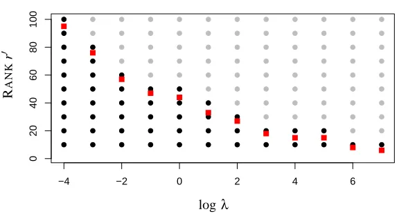
The MMMF criterion (27) defines a two-dimensional family of models indexed by(r′,λ), while the SOFT-IMPUTEcriterion (28) defines a one-dimensional family. In light of Theorem 3, this family is a special path in the two-dimensional grid of solutions[_Uˆ_(r′_,λ),Vˆ_(r′_,λ)].Figure 1 depicts the situation. Any MMMF model at parameter combinations above the red squares are redundant, since their fit is the same at the red square. However, in practice the red squares are not known to MMMF, nor is the actual rank of the solution. Further orthogonalization of ˆU and ˆV would be required to reveal

the rank, which would only be approximate (depending on the convergence criterion of the MMMF algorithm).

Despite the equivalence of (27) and (28) when r′=min(m,n), the criteria are quite different. While (28) is a convex optimization problem in Z, (27) is a non-convex problem in the variables

U,V and has possibly several local minima; see also Abernethy et al. (2009). It has been observed

empirically and theoretically (Burer and Monteiro, 2005; Rennie and Srebro, 2005) that bi-convex methods used in the optimization of (27) can get stuck in sub-optimal local minima for a small value of r′ or a poorly chosen starting point. For a large number of factors r′and large dimensions m,n

the computational cost may be quite high (See also experimental studies in Section 9.2).

Criterion (28) is convex in Z for every value ofλ, and it outputs the solution ˆZ in the form of

its soft-thresholded SVD, implying that the “factors” U,V are already orthogonal and the rank is

−4 −2 0 2 4 6

0

20

40

60

80

100

R

A

N

K

r

′

logλ

Figure 1: Comparison of the parameter space for MMMF (grey and black points), and SOFT -IMPUTE(red squares) for a simple example. Since all MMMF solutions with parameters above the red squares are identical to the SOFT-IMPUTEsolutions at the red squares, all the grey points are redundant.

MMMF has two different tuning parameters r′ and λ, both of which are related to the rank or spectral properties of the matrices U,V . SOFT-IMPUTEhas only one tuning parameterλ. The

presence of two tuning parameters is problematic:

• It results in a significant increase in computational burden, since for every given value of r′, one needs to compute an entire system of solutions by varyingλ(see Section 9 for illustra-tions).

• In practice when neither the optimal values of r′andλare known, a two-dimensional search (for example, by cross validation) is required to select suitable values.

Further discussions and connections between the tuning parameters and spectral properties of the matrices can be found in Burer and Monteiro (2005) and Abernethy et al. (2009).

The proof of Theorem 3 requires a lemma.

Lemma 6 For any matrix Z, the following holds:

||Z||∗= min

U,V : Z=UVT 1 2 kUk

2

F+kVk2F

. (29)

If rank(Z) =k≤min{m,n}, then the minimum above is attained at a factor decomposition Z= Um×kVnT×k.

Note that in the decomposition Z=UVT in (29) there is no constraint on the number of columns r of the factor matrices Um×rand Vn×r.Lemma 6 is stronger than similar results appearing in Rennie

8.1 Proof of Theorem 3

Part 1. For r=min(m,n), any matrix Zm×ncan be written in the form of Z =UVT.The criterion

(27) can be written as

min

U,V 1

2||PΩ(X−UV T_)||2

F+λ2(kUk 2

F+kVk2F) (30)

=min

U,V

1

2||PΩ(X−UVT)||F2+λkUVTk∗ (by Lemma 6)

=min

Z

1

2||PΩ(X−Z)||F2+λkZk∗. (31)

The equivalence of the criteria in (30) and (31) completes the proof of part 1.

Part 2. Note that if we know that the solution ˆZ∗to (28) withλ=λ∗_{has rank r}∗_{, then ˆZ}∗_{also solves}

min

Z,rank(Z)=r∗

1

2||PΩ(X−Z)||2F +λkZk∗.

We now repeat the steps (30)—(31), restricting the rank r′ of U and V to be r′=r∗, and the result follows.

9. Numerical Experiments and Comparisons

In this section we study the performance of SOFT-IMPUTE, its post-processed variants, and HARD -IMPUTE for noisy matrix completion problems. The examples assert our claim that the matrix reconstruction criterion (4) (Cai et al., 2008) is too rigid if one seeks good predictive models. We include the related procedures of Rennie and Srebro (2005) and Keshavan et al. (2009) in our com-parisons.

The reconstruction algorithm OPTSPACE, described in Keshavan et al. (2009) considers crite-rion (1) (in the presence of noise). It uses the representation Z=U SV′(which need not correspond to the SVD). OPTSPACEalternates between estimating S and U,V (in a Grassmann manifold) for

computing a rank-r decomposition ˆZ=_{U ˆ}ˆ_{S ˆV}′_{. It starts with a sparse SVD on a clean version of the}

observed matrix PΩ(X).This is similar to the formulation of MMMF (27) as detailed in Section 8, without the squared Frobenius norm regularization on the components U,V .

To summarize, we study the following methods:

1. SOFT-IMPUTE–Algorithm 1;

2. SOFT-IMPUTE+–post-processing on the output of SOFT-IMPUTE, as in Section 7;

3. HARD-IMPUTE–Algorithm 2, starting with the output of SOFT-IMPUTE+;

4. SVT–algorithm by Cai et al. (2008);

5. OPTSPACE–reconstruction algorithm by Keshavan et al. (2009);

In all our simulation studies we use the underlying model Zm×n=Um×rVr′×n+ε, where U and V are

random matrices with standard normal Gaussian entries, and εis i.i.d. Gaussian. Ωis uniformly random over the indices of the matrix with p% percent of missing entries. These are the models under which the coherence conditions hold true for the matrix completion problem to be meaningful (Cand`es and Tao, 2009; Keshavan et al., 2009). The signal to noise ratio for the model and the test-error (standardized) are defined as

SNR=

s

var(UV′₎

var(ε) ; Test Error=

kP_Ω⊥(UV′_{−Z)ˆ k}2 F

kP_Ω⊥(UV′_)k2 F

.

Training error (standardized) is defined as

Training Error=kPΩ(Z−Z)ˆ k 2 F

kPΩ(Z)k2 F

,

the fraction of the error explained on the observed entries by the estimate relative to a zero estimate. Figures 2, 3 and 4 show training and test error for all of the algorithms mentioned above—both as a function of nuclear norm and rank—for the three problem instances. The results displayed in the figures are averaged over 50 simulations, and also show one-standard-error bands (hardly visible). In all examples(m,n) = (100,100).For MMMF we use r′=min(m,n) =100, the number of columns in U and V . The performance of MMMF is displayed only in the plots with the nuclear norm along the horizontal axis, since the algorithm does not deliver a precise rank. SNR, true rank and percentage of missing entries are indicated in the figures. There is a unique correspondence betweenλand nuclear norm. The plots versus rank indicate how effective the nuclear norm is as a rank approximation—that is whether it recovers the true rank while minimizing prediction error.

For routines not our own we use the MATLAB code as supplied on webpages by the authors. For SVT second author of Cai et al. (2008), for OPTSPACEthird author of Keshavan et al. (2009), and for MMMF first author of Rennie and Srebro (2005).

9.1 Observations

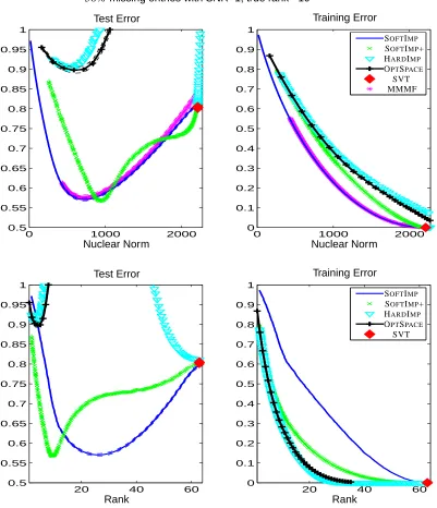
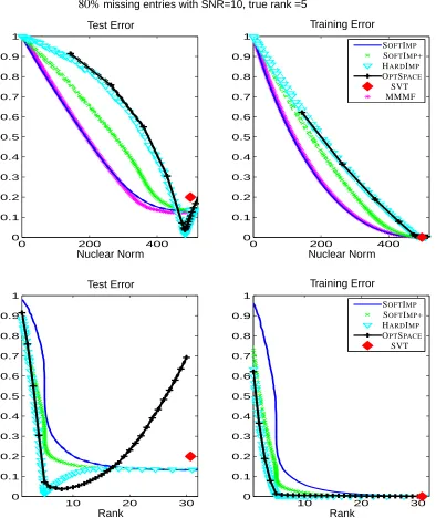
The captions of each of Figures 2–4 detail the results, which we summarize here. For the first two figures, the noise is quite high with SNR=1, and 50% of the entries are missing. In Figure 2 the true rank is 10, while in Figure 3 it is 6. SOFT-IMPUTE, MMMF and SOFT-IMPUTE+ have the best prediction performance, while SOFT-IMPUTE+ is better at estimating the correct rank. The other procedures perform poorly here, although OPTSPACE improves somewhat in Figure 3. SVT has very poor prediction error, suggesting once again that exactly fitting the training data is far too rigid. SOFT-IMPUTE+ has the best performance in Figure 3 (smaller rank—more aggressive fitting), and HARD-IMPUTEstarts recovering here. In both figures the training error for SOFT-IMPUTE (and hence MMMF) wins as a function of nuclear norm (as it must, by construction), but the more aggressive fitters SOFT-IMPUTE+ and HARD-IMPUTEhave better training error as a function of rank.

Though the nuclear norm is often viewed as a surrogate for the rank of a matrix, we see in these examples that it can provide a superior mechanism for regularization. This is similar to the performance ofLASSOin the context of regression. Although theLASSOpenalty can be viewed as a

convex surrogate for theℓ0penalty in model selection, itsℓ1penalty provides a smoother and often

50%missing entries with SNR=1, true rank =10

0 1000 2000

0.5 0.55 0.6 0.65 0.7 0.75 0.8 0.85 0.9 0.95 1

0 1000 2000

0 0.1 0.2 0.3 0.4 0.5 0.6 0.7 0.8 0.9 1

Training Error Test Error

Nuclear Norm Nuclear Norm

SOFTIMP OPTSPACE

SVT MMMF HARDIMP SOFTIMP+

20 40 60

0.5 0.55 0.6 0.65 0.7 0.75 0.8 0.85 0.9 0.95 1

20 40 60

0 0.1 0.2 0.3 0.4 0.5 0.6 0.7 0.8 0.9 1

Training Error Test Error

Rank Rank

SOFTIMP OPTSPACE

SVT HARDIMP SOFTIMP+

Figure 2: SOFTIMP+ refers to the post-processing after SOFT-IMPUTE; HARD-IMPUTEuses SOFT

-IMP+ as starting values. Both SOFT-IMPUTEand SOFT-IMPUTE+ perform well (predic-tion error) in the presence of noise; the latter estimates the actual rank of the matrix. MMMF (with full rank 100 factor matrices) has performance similar to SOFT-IMPUTE.

50%missing entries with SNR=1, true rank =6

0 500 1000 1500

0.3 0.4 0.5 0.6 0.7 0.8 0.9 1

0 500 1000 1500

0 0.1 0.2 0.3 0.4 0.5 0.6 0.7 0.8 0.9

Training Error Test Error

Nuclear Norm Nuclear Norm

SOFTIMP OPTSPACE

SVT MMMF HARDIMP SOFTIMP+

20 40 60

0.3 0.4 0.5 0.6 0.7 0.8 0.9 1

20 40 60

0 0.1 0.2 0.3 0.4 0.5 0.6 0.7 0.8 0.9

Training Error Test Error

Rank Rank

SOFTIMP OPTSPACE

SVT HARDIMP SOFTIMP+

Figure 3: SOFT-IMPUTE+ has the best prediction error, closely followed by SOFT-IMPUTE and

80%missing entries with SNR=10, true rank =5

0 200 400

0 0.1 0.2 0.3 0.4 0.5 0.6 0.7 0.8 0.9 1

0 200 400

0 0.1 0.2 0.3 0.4 0.5 0.6 0.7 0.8 0.9 1

Training Error Test Error

Nuclear Norm Nuclear Norm

SOFTIMP OPTSPACE

SVT MMMF HARDIMP SOFTIMP+

10 20 30

0 0.1 0.2 0.3 0.4 0.5 0.6 0.7 0.8 0.9 1

10 20 30

0 0.1 0.2 0.3 0.4 0.5 0.6 0.7 0.8 0.9 1

Training Error Test Error

Rank Rank

SOFTIMP OPTSPACE

SVT HARDIMP SOFTIMP+

Figure 4: With low noise the performance of HARD-IMPUTE improves. It gets the correct rank

whereas OPTSPACE slightly overestimates the rank. HARD-IMPUTE has the best pre-diction error, followed by OPTSPACE. Here MMMF has slightly better prediction error than SOFT-IMPUTE. Although the noise is low here, SVT recovers a matrix with high

In Figure 4 with SNR=10 the noise is relatively small compared to the other two cases. The true underlying rank is 5, but the proportion of missing entries is much higher at eighty percent. Test errors of both SOFT-IMPUTE+ and SOFT-IMPUTEare found to decrease till a large nuclear norm after which they become roughly the same, suggesting no further impact of regularization. MMMF has slightly better test error than SOFT-IMPUTE around a nuclear norm of 350, while in theory they should be identical. Notice, however, that the training error is slightly worse (everywhere), suggesting that MMMF is sometimes trapped in local minima. The fact that this slightly underfit solution does better in test error is a quirk of this particular example. OPTSPACEperforms well in this high-SNR example, achieving a sharp minima at the true rank of the matrix. HARD-IMPUTE

performs the best in this example. The better performance of both OPTSPACEand HARD-IMPUTE

over SOFT-IMPUTEcan be attributed both to the low-rank truth and the high SNR. This is reminis-cent of the better predictive performance of best-subset or concave penalized regression often seen overLASSOin setups where the underlying model is very sparse (Friedman, 2008).

9.2 Comparison with Fast MMMF (Rennie and Srebro, 2005)

In this section we compare SOFT-IMPUTEwith MMMF in terms of computational efficiency. We also examine the consequences of two regularization parameters (r′,λ) for MMMF over one for SOFT-IMPUTE.

Rennie and Srebro (2005) describes a fast algorithm based on conjugate-gradient descent for minimization of the MMMF criterion (6). With (6) being non-convex, it is hard to provide theo-retical optimality guarantees for the algorithm for arbitrary r′,λ—that is, what type of solution it converges to or how far it is from the global minimizer.

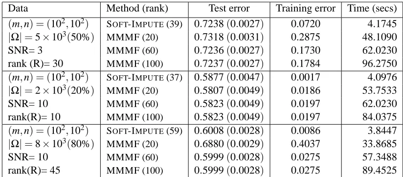
In Table 1 we summarize the performance results of the two algorithms. For both SOFT-IMPUTE

and MMMF we consider a equi-spaced grid of 150λ∈[λmin,λmax],withλmincorresponding to a

full-rank solution of SOFT-IMPUTEandλmaxthe zero solution. For MMMF, three different values

of r′were used, and for each(_Uˆ_,Vˆ_{)were solved for over the grid ofλvalues. A separate held-out} validation set with twenty percent of the missing entries sampled fromΩ⊥ were used to train the tuning parameterλ(for each value of r′) for MMMF and SOFT-IMPUTE. Finally we evaluate the standardized prediction errors on a test set consisting of the remaining eighty percent of the missing entries in Ω⊥. In all cases we report the training errors and test errors on the optimally tuned λ. SOFT-IMPUTEwas run till a tolerance of 10−4 was achieved (fraction of decrease of objective value). Likewise for MMMF we set the tolerance of the conjugate gradient method to 10−4.

Data Method (rank) Test error Training error Time (secs)

(m,n) = (102,102) SOFT-IMPUTE(39) 0.7238(0.0027) 0.0720 4.1745 |Ω|=5×103(50%) MMMF (20) 0.7318(0.0031) 0.2875 48.1090

SNR= 3 MMMF (60) 0.7236(0.0027) 0.1730 62.0230

rank (R)= 30 MMMF (100) 0.7237(0.0027) 0.1784 96.2750

(m,n) = (102,102) SOFT-IMPUTE(37) 0.5877(0.0047) 0.0017 4.0976 |Ω|=2×103(20%) MMMF (20) 0.5807(0.0049) 0.0186 53.7533

SNR= 10 MMMF (60) 0.5823(0.0049) 0.0197 62.0230

rank(R)= 10 MMMF (100) 0.5823(0.0049) 0.0197 84.0375

(m,n) = (102,102) SOFT-IMPUTE(59) 0.6008(0.0028) 0.0086 3.8447 |Ω|=8×103(80%) MMMF (20) 0.6880(0.0029) 0.4037 33.8685

SNR= 10 MMMF (60) 0.5999(0.0028) 0.0275 57.3488

rank(R)= 45 MMMF (100) 0.5999(0.0028) 0.0275 89.4525

Table 1: Performances of SOFT-IMPUTEand MMMF for different problem instances, in terms of test error (with standard errors in parentheses), training error and times for learning the models. SOFT-IMPUTE,“rank” denotes the rank of the recovered matrix, at the optimally chosen value ofλ. For the MMMF, “rank” indicates the value of r′in Um×r′,Vn×r′. Results

are averaged over 50 simulations.

exploiting the specialized Sparse+Low-Rank structure (22). We report our findings on one such simulation example:

• For(m,n) = (2000,1000),|Ω|/(m·n) =0.2, rank=500 and SNR=10; SOFT-IMPUTEtakes 1.29 hours to compute solutions on a grid of 100λvalues. The test error on the validation set and training error are 0.9630 and 0.4375 with the recovered solution having a rank of 225.

For the same problem, MMMF with r′=200 takes 6.67 hours returning a solution with test-error 0.9678 and training test-error 0.6624. With r′=400 it takes 12.89 hrs with test and training errors 0.9659 and 0.6564 respectively.

We will like to note that DeCoste (2006) proposed an efficient implementation of MMMF via an ensemble based approach, which is quite different in spirit from the batch optimization algorithms we are studying in this paper. Hence we do not compare it withSOFT-IMPUTE.

9.3 Comparison with Nesterov’s Accelerated Gradient Method

Ji and Ye (2009) proposed a first-order algorithm based on Nesterov’s acceleration scheme (Nes-terov, 2007), for nuclear norm minimization for a generic multi-task learning problem (Argyriou et al., 2008, 2007). Their algorithm (Liu et al., 2009; Ji and Ye, 2009) can be adapted to the SOFT -IMPUTEproblem (10); hereafter we refer to it as NESTEROV. It requires one to compute the SVD of

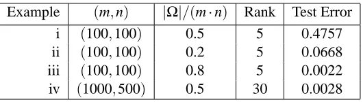
Since both algorithms solve the same criterion, the quality of the solutions—objective values, training and test errors—will be the same (within tolerance). We hence compare their performances based on the times taken by the algorithms to converge to the optimal solution of (10) on a grid of values ofλ.Both algorithms compute a path of solutions using warm starts. Results are shown in Figure 5, for four different scenarios described in Table 2.

Example (m,n) |Ω|/(m·n) Rank Test Error

i (100,100) 0.5 5 0.4757

ii (100,100) 0.2 5 0.0668 iii (100,100) 0.8 5 0.0022 iv (1000,500) 0.5 30 0.0028

Table 2: Four different examples used for timing comparisons of SOFT-IMPUTE and NESTEROV

(accelerated Nesterov algorithm of Ji and Ye 2009). In all cases the SNR=10.

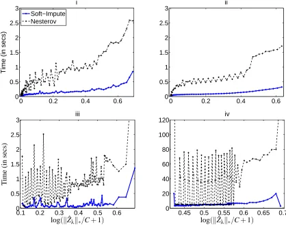
Figure 5 shows the time to convergence for the two algorithms. Their respective number of iterations are not comparable. This is because NESTEROVuses a line-search to compute an adaptive step-size (approximate the Lipschitz constant) at every iteration, whereas SOFT-IMPUTEdoes not.

SOFT-IMPUTEhas a rate of convergence given by Theorem 2, which for large k is worse than the accelerated version NESTEROVwith rate O(1/k2). However, timing comparisons in Figure 5 show thatSOFT-IMPUTEperforms very favorably. We do not know the exact reason behind this, but mention some possibilities. Firstly the rates are worst case convergence rates. On particular problem instances of the form (10), the rates of convergence in practice of SOFT-IMPUTEand NESTEROV

may be quite similar. Since Ji and Ye (2009) uses an adaptive step-size strategy, the choice of a step-size may be time consuming. SOFT-IMPUTEon the other hand, uses a constant step size.

Additionally, it appears that the use of the momentum term in NESTEROVaffects the

Sparse+Low-rank decomposition (22). This may prevent the algorithm to be adapted for solving large problems,

due to costly SVD computations.

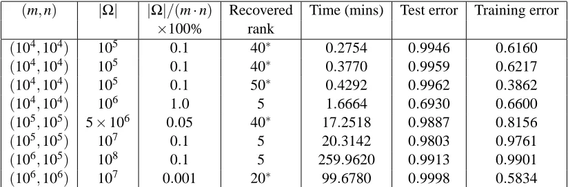
9.4 Large Scale Simulations for SOFT-IMPUTE

Table 3 reports the performance of SOFT-IMPUTEon some large-scale problems. All computations are performed in MATLAB and the MATLAB implementation of PROPACK is used. Data input, access and transfer in MATLAB take a sizable portion of the total computational time, given the size of these problems. However, the main computational bottle neck in our algorithm is the struc-tured SVD computation. In order to focus more on the essential computational task, Table 3 displays the total time required to perform the SVD computations over all iterations of the algorithm. Note that for all the examples considered in Table 3, the implementations of algorithms NESTEROV(Liu et al., 2009; Ji and Ye, 2009) and MMMF (Rennie and Srebro, 2005) are prohibitively expensive both in terms of computational time and memory requirements, and hence could not be run. We used the value λ=||P_Ω(X)||2/K with SOFT-IMPUTE, with K=1.5 for all examples but the last,

where K=2. λ0=||PΩ(X)||2is the largest singular value of the input matrix X (padded with

ze-ros); this is the smallest value ofλfor which S_λ0(PΩ(X)) =0 in the first iteration of SOFT-IMPUTE

0 0.2 0.4 0.6 0

0.5 1 1.5 2 2.5 3

Soft−Impute Nesterov

T

im

e

(i

n

s

e

c

s

)

i

0 0.2 0.4 0.6

0 0.5 1 1.5 2 2.5

3 ii

0.1 0.2 0.3 0.4 0.5 0.6

0 0.5 1 1.5 2 2.5 3

T

ime

(in

se

cs

)

iii

log(k_Zˆ_λk∗/C+1) 0.45 0.5 0.55 0.6 0.65 0.7 0

20 40 60 80 100

120 iv

log(k_Zˆ_λk∗/C+1)

Figure 5: Timing comparisons of SOFT-IMPUTEand NESTEROV(accelerated Nesterov algorithm of Ji and Ye 2009). The horizontal axis corresponds to the standardized nuclear norm, with C=max_λk_Zˆ_{λk∗. Shown are the times till convergence for the two algorithms over} an entire grid ofλvalues for examples i–iv (in the last the matrix dimensions are much larger). The overall time differences between Examples i–iii and Example iv is due to the increased cost of the SVD computations. Results are averaged over 10 simulations. The times for NESTEROVchange far more erratically withλthan they do for SOFT-IMPUTE.

The prediction performance is awful for all but one of the models, because in most cases the fraction of observed data is very small. These simulations were mainly to show the computational capabilities of SOFT-IMPUTEon very large problems.

10. Application to the Netflix Data Set

(m,n) |Ω| |Ω|/(m·n) Recovered Time (mins) Test error Training error

×100% rank

(104,104_{) 10}5 _{0.1 40}∗ _{0.2754 0.9946 0.6160} (104,104_{) 10}5 _{0.1 40}∗ _{0.3770 0.9959 0.6217} (104,104_{) 10}5 _{0.1 50}∗ _{0.4292 0.9962 0.3862}

(104,104_{) 10}6 _{1.0 5 1.6664 0.6930 0.6600}

(105_,105_{) 5×10}6 _{0.05 40}∗ _{17.2518 0.9887 0.8156}

(105,105_{) 10}7 _{0.1 5 20.3142 0.9803 0.9761}

(106,105_{) 10}8 _{0.1 5 259.9620 0.9913 0.9901}

(106_,106_{) 10}7 _{0.001 20}∗ _{99.6780 0.9998 0.5834}

Table 3: Performance of SOFT-IMPUTEon different problem instances. All models are generated with SNR=10 and underlying rank=5. Recovered rank is the rank of the solution matrix

ˆ

Z at the value ofλused in (10). Those with stars reached the “maximum rank” threshold, and option in our algorithm. Convergence criterion is taken as “fraction of improvement of objective value” less than 10−4or a maximum of 15 iterations for the last four examples. All implementations are done in MATLAB including the MATLAB implementation of PROPACK on a Intel Xeon Linux 3GHz processor.

ratings was distributed to participants, for calibration purposes. The movies and customers in the qualifying, test and probe sets are all subsets of those in the training set.

The ratings are integers from 1 (poor) to 5 (best). Netflix’s own algorithm has an RMSE of 0.9525, and the contest goal was to improve this by 10%, or an RMSE of 0.8572 or better. The contest ran for about 3 years, and the winning team was “Bellkor’s Pragmatic Chaos”, a merger of three earlier teams (seehttp://www.netflixprize.com/for details). They claimed the grand prize of $1M on September 21, 2009.

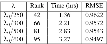
Many of the competitive algorithms build on a regularized low-rank factor model similar to (6) using randomization schemes like mini-batch, stochastic gradient descent or sub-sampling to reduce the computational cost over making several passes over the entire data-set (see Salakhutdinov et al., 2007; Bell and Koren., 2007; Takacs et al., 2009, for example). In this paper, our focus is not on using randomized or sub-sampling schemes. Here we demonstrate that our nuclear-norm regular-ization algorithm can be applied in batch mode on the entire Netflix training set with a reasonable computation time. We note however that the conditions under which the nuclear-norm regulariza-tion is theoretically meaningful (Cand`es and Tao, 2009; Srebro et al., 2005a) are not met on the Netflix data set.

λ Rank Time (hrs) RMSE λ0/250 42 1.36 0.9622

λ0/300 66 2.21 0.9572

λ0/500 81 2.83 0.9543

λ0/600 95 3.27 0.9497

Table 4: Results of applying SOFT-IMPUTEto the Netflix data. λ0=||PΩ(X)||2; see Section 9.4.

The computations were done on a Intel Xeon Linux 3GHz processor; timings are reported based on MATLAB implementations of PROPACK and our algorithm. RMSE is root-mean squared error, as defined in the text.

Acknowledgments

We thank the reviewers for their suggestions that lead to improvements in this paper. We thank Stephen Boyd, Emmanuel Candes, Andrea Montanari, and Nathan Srebro for helpful discussions. Trevor Hastie was partially supported by grant DMS-0505676 from the National Science Founda-tion, and grant 2R01 CA 72028-07 from the National Institutes of Health. Robert Tibshirani was partially supported from National Science Foundation Grant DMS-9971405 and National Institutes of Health Contract N01-HV-28183.

Appendix A. Proofs

We begin with the proof of Lemma 1.

A.1 Proof of Lemma 1

Proof Let Z=_U˜_m×nD˜_n×nV˜′

n×nbe the SVD of Z.Assume without loss of generality, m≥n. We will

explicitly evaluate the closed form solution of the problem (8). Note that

1

2kZ−Wk

2

F+λkZk∗=

1 2

(

kZk2 F−2

n

∑

i=1

˜

diu˜′iW ˜vi+ n

∑

i=1

˜

d2_i

)

+λ

n

∑

i=1

˜

di (32)

where

˜

D=diagd˜1, . . . ,d˜n

, U˜ = [u˜1, . . . ,u˜n], V˜ = [v˜1, . . . ,v˜n].

Minimizing (32) is equivalent to minimizing

−2

n

∑

i=1

˜

diu˜′iW ˜vi+ n

∑

i=1

˜

d_i2+

n

∑

i=1

2λd˜i; w.r.t.(u˜i,v˜i,d˜i),i=1, . . . ,n,

under the constraints ˜U′U˜ =In,V˜′V˜ =Inand ˜di≥0 ∀i.

Observe the above is equivalent to minimizing (w.r.t. ˜U,V ) the function Q(˜ U˜,V˜):

Q(_U˜_,V˜_{) =min}

˜ D≥0

1 2 ( −2 n

∑

i=1

˜

diu˜′iW ˜vi+ n

∑

i=1

˜

d_i2

)

+λ

n

∑

i=1

˜