Energy Efficient Fault Tolerant Sensor Node Failure Detection in WSNs

(1)

Energy Efficient Fault Tolerant Sensor Node Failure Detection in WSNs

Ravindra Duche

1,*

, Nisha Sarwade

2

1

Department of Electronics and Telecommunication Engineering, LTCOE, Mumbai,

Maharashtra, India.

2

Department

o

f Electrical Engineering,

VJTI, Mumbai, Maharashtra, India.

Received 03 November 2015; received in revised form 11 March 2016; accepted 15 June 2016

Abstract

In WSNs, the large numbers of portable sensor nodes are deployed randomly and can fail due to battery problem,

environmental conditions or are unattended. Faulty sensor node detection techniques are mainly affected due to

energy consumption of sensor nodes in WSNs. Therefore, the primary goal of this investigation is to design energy

efficient fault tolerant sensor node failure detection. A faulty sensor node is detected by measuring the Round Trip

Delay (RTD) times of Round Trip Paths (RTPs) in WSNs. Fault tolerance is achieved by assigning unique source

node or Cluster Head (CH) for each RTP in WSNs. Energy consumed by individual sensor node is minimized due to

optimal involvement of sensor nodes in the detection process. The proposed method is implemented and tested on

WSNs with six sensor nodes.

Keywords: Faultytolerance, RTD, Energy efficient, RTPs, Unique source node, WSNs.

1. Introduction

Portable wireless sensor nodes are positioned randomly in wireless sensor networks (WSNs) [1-2]. These sensor nodes can

get faulty because of environment, communication module or power supply related problem [2-4]. Probability of wireless sensor

nodes failure is mainly due to limited battery energy. The regular manual maintenance of such sensor nodes will be troublesome.

As a result fault detection and fault recovery becomes much important in case of WSNs. Lifetime of WSNs degrades due to

faulty sensor nodes. In order to minimize the faults to improve the lifetime of WSNs; fault tolerance has to be incorporated.

Fault tolerance is the ability to ensure the functionality of the network in the events of faults and failures. Due to

deployment of portable wireless sensor nodes in hostile and un-attended environment faults and failures are normal facts,

therefore fault tolerance and reliable data transmission is of great importance [10, 14-19]. Fault detection technique used in

wireless network consumes significant power hence will reduce the life of a sensor node ultimately causing its failure [5].

Energy consumption of sensor in wireless network depends upon the time delay, as there is trade-off between energy and

time delay [6]. Lifetime of WSNs depends upon the lifetime of sensor node. It can be determined as the time from the

deployment to non-functioning of wireless sensor network. Non-functioning of WSNs can be estimated as the first sensor node

die or percentage of sensor node dies or loss of coverage. Lifetime of wireless network will be increased by reducing the energy

consumed by sensor node during fault detection [6,15]. Energy hole aware energy efficient communication routing algorithm

(EHAEC) proposed in [19] is useful to avoid the single faulty sensor node in WSN. Redundant communication routes are

(2)

identified by using the EHAEC tree which is used to tolerate the failure of one node. Here sensor energy is minimized by

generating an energy efficient spanning tree.A fuzzy logic based mechanism that determine the sleeping time of field devices in

a home automation environment based on Bluetooth Low Energy (BLE) is proposed in [18]. Here sensor node efficiency is

improved by using low power device like Bluetooth and fuzzy logic based algorithm.

Link failure detection with the help of monitoring cycles and monitoring paths is presented in [8]. It has limitations due to

necessity of three-edge connectivity for each node as well as use of separate wavelength for each monitoring cycle and

monitoring locations. Cluster head (CH) rotation and load balancing technique is used in [9] and [10] to achieve fault tolerance.

This technique suffers due to data loss, frequent re-clustering and continuous evaluation of received signal strength (RSS). Also

failure of cluster head causes more damage to system because of permanent loss of data during its rotation. In [7] time delay

estimation (TDE) technique is used to detect the faulty sensor. Analysis of TDE is complex and may results in wrong estimation

due to triangularity test failure.

In our earlier work [11], Round Trip Delay (RTD) time of Round Trip Paths (RTPs) is measured and compared to detect the

faulty sensor node in WSNs. Here depending upon the RTD time of RTPs, faulty sensor node is first located and then it is

identified as failed or malfunctioning. Scalability and reliability of this method is tested and verified by implementing it both in

hardware and software.

Further to address the issues of fault tolerance and energy consumption in our fault detection scheme, we have focused our

study on selection of RTPs. Proposed method is implemented to circular, rectangular and triangular topologies of WSNs to

examine its performance. The paper is organized into five sections. In Section II, fault tolerance with energy savings approach is

described. In Section III, implementation of this scheme to other topologies like rectangular and triangular is demonstrated.

Experimental results for failed as well as malfunctioning behaviour of sensor node are presented in section IV. Section V

concludes the paper.

2. Fault Tolerant and Energy Saving Approach

Numbers of RTPs used in fault detection decides the energy consumed by individual sensor node. Minimal involvement of

individual sensor node in RTPs will curtail energy consumed by it. Simultaneously, fault tolerance is determined by the numbers

of RTPs in WSNs. In order to achieve fault tolerance as well as minimum energy consumption by sensor node in fault detection,

RTPs equal to the number of sensor nodes in WSNs are selected. These specially selected RTPs are called as Linear RTPs.

Linear RTPs have effectively managed the less contribution of individual sensor node in fault detection to save the energy. At

the same time, monitoring and detection of fault is distributed among the source nodes of RTPs, thereby achieves fault tolerance.

Lifetime of source node or cluster head in RTPs is enhanced due to distribution of computational load among them.

2.1 Proposed Fault-Tolerant Technique

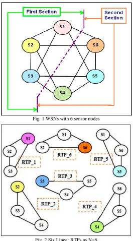
The circular topology WSNs as shown in Fig.1 is used to demonstrate the fault detection using RTD time measurements of

RTPs. For this topology experimental results of hardware and software are described in our earlier paper [11]. Initially the

wireless network is scaled into linear RTPs; here six linear RTPs will form because circular WSNs have six sensor nodes. Six

linear RTPs i.e. RTP_1 to RTP_6 are shown in Fig.2. Each RTP has unique source node, hence detection process is equally

(3)

Fig. 1 WSNs with 6 sensor nodes

Fig. 2 Six Linear RTPs as N=6

Now the entire network is divided into two sections as indicated in Fig.1. First section consists of three linear RTPs i.e.

RTP_1, 2 and 3 and second section consists of remaining three linear RTPs i.e. RTPs_4, 5 and 6 respectively. Since RTP_1 and

RTP_4 have separate source nodes, parallel analysis of RTD time is feasible. This will save the overall analysis time. RTP_1 is

formed with sensor nodes 1, 2 and 3, whose analysis will assist us to determine the fault present at sensor nodes 1, 2 and 3

respectively. Similar analysis of RTP_4 will assist us to determine the fault present at sensor nodes 4, 5 and 6.

The algorithm to detect the working as well as faulty sensor node is explained below. The discrete RTPs with three sensor

nodes explained in Fig. 3 below are used to determine the fault in WSNs. Discrete RTPs are selected by incrementing the source

node value by three and their respective RTD times are measured by using the subroutine. The highest value of RTD time

(4)

Main Program: Discrete RTPs selection and there analysis to detect faulty sensor node [13]

1. Select any sensor node SX from WSN with N sensor nodes,

The value of X = 1, 2, 3…….N (∴ S1 ≤ SX ≤ SN).

2. RTP_X formed has sensor sequence as SX –SX+1 – SX+2.

3. Call subroutine “RTD Time”.

Subroutine: RTD Time

a) If SX+1 =SN then replace SX+2 by S1

Else if SX+1 >SN then replace SX+1 by S1 and SX+2 by

S2 respectively.

b) Measure the round trip delay time of corresponding RTP. Initially it is RTP_X.

c) Return to main program.

4. If τRTD_X = τTHR then Increment SX by 3(∴ SX =SX+3)

If SX+3 >SN then reset SX+3 to SN and go to step 2

Else go to step 2

Else Call subroutine “RTD Time”. Measure RTD time of RTP_(X+1) having sequence as S

X+1– SX+2– SX+3.

5. If τRTD_(X+1) = τTHR then go to step 7

Else if τRTD_X = ∞ then SX node is failed (dead).

Otherwise SX node is malfunctioning.

6. Go to step 4

7. Call Subroutine “RTD Time”. Measure RTD time of RTP_(X+2) having sequence as SX+2 – SX+3– SX+4.

8. If τRTD_(X+2) = τTHR then go to step 10

Else if τRTD_(X+1) = ∞ then SX+1 node is failed (dead)

Otherwise SX+1 node is malfunctioning

9. Go to step 4

10. If τRTD_(X+2) = ∞ then SX+2 node is failed (dead)

Otherwise SX+2 node is malfunctioning

11. If SX+2 >SN then go to step 4

12. Stop.

In the first stage of fault detection process, the RTP_1 and RTP_4 as shown in Fig.3 are examined simultaneously. If the

RTD times of both RTPs are less than the threshold value then all sensor nodes in network are verified as functioning

appropriately. In this analysis, if RTD time of any RTP is higher than the threshold value then a fault exists in it. Now to locate

this fault, second stage of analysis is performed on this particular RTP. In the second stage the RTD time of remaining two RTPs

are measured and compared with the threshold value.

(5)

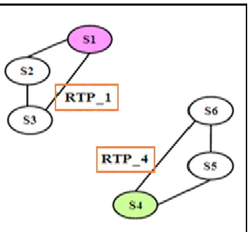
The RTP_2 and RTP_3 shown in Fig.4 are examined if RTD time of RTP_1 is found to be higher than the threshold value.

Similarly RTP_5 and RTP_6 as shown in Fig.5 are examined if RTD time of RTP_4 is found to be higher than the threshold

value. Depending upon the results of RTD time of RTPs in the second stage, particular fault is located. After this, in the last

stage, nature of fault either failed or malfunctioning is verified. This is done by observing the RTD time value of RTP in which

fault is located, if it is infinity then the faulty sensor node is failed otherwise (higher than the threshold value) it is

malfunctioning.

Fig. 4 RTPs examined in second stage if fault is detected in RTP_1 during first stage

Fig. 5 RTPs examined in second stage if fault is detected in RTP_4 during first stage

In this way fault is located and detected in WSN with the help of RTD time of RTPs. At each stage of examination separate

sensor node (i.e. source node of RTP) is involved in fault detection. Hence computational load of single cluster head or sensor

node is minimized by distributing it to other sensor nodes in WSN. In this way distribution of fault detection task to various

sensor nodes in WSN will provide the fault tolerance

2.2 Energy Saving Approach

Energy consumed by sensor node in WSNs can be divided into two categories: primary energy which is required for basic

operation of sensor node to sense the physical quantity and the secondary energy, which is the additional energy, required by

sensor node during the fault detection process in WSN. Energy consumed by individual sensor node in proposed method depends

upon number of RTPs and numbers of sensor nodes in each RTP. Less contribution of sensor node is achieved by selecting linear

(6)

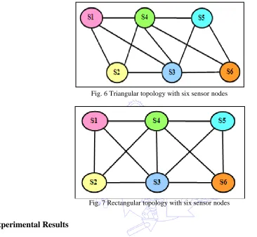
2.3 Implementation with other topologies of WSNs

In order to verify the applicability of the fault detection methodology implemented in circular topology, other topologies of

WSNs like triangular and rectangular are selected to verify it. Triangular as well as rectangular topologies with six sensor nodes

are shown in Fig.6 and 7 respectively. The round trip distance in RTP will vary according to the topology even if the sensors are

kept at equal distance from each other. The round trip distances for triangular, rectangular and circular topologies are 3.0, 3.4 and

3.8 feet respectively; when nearby sensor nodes in RTP are 1 foot apart.

Fig. 6 Triangular topology with six sensor nodes

Fig. 7 Rectangular topology with six sensor nodes

3. Experimental Results

Wireless sensor nodes are implemented by using ATMEGA16L and XBEE S2 module. Linear RTPs are configured and

simulated in real time by using X-CTU and Dock light V1.9 software’s respectively. Details of configuration, simulation, RTD

time measurements of RTPs and subsequent faulty sensor node detection with experimental results are described in our earlier

paper [11].

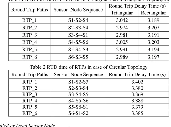
3.1 Estimation of Threshold RTD time in WSN

Since the RTD time of RTP is the linear function of distance between sensor nodes [13], the threshold RTD time for RTP in

three topologies will be different. As faulty sensor node detection is based on comparison of instantaneous and threshold RTD

times, therefore determination of threshold RTD time for each topology is essential. Sensor node sequence in RTP will differ

according to the topology orientation. As sensor node sequence of linear RTPs in triangular and rectangular topologies are

identical, their RTD time results are mentioned in Table 1. But in case of circular topology sensor node sequence differs hence

its RTD time results are shown in Table 2. Referring Tables 1 and 2, the threshold RTD time (highest RTD time of a RTP) for

(7)

Table 1 RTD time of RTPs in case of Triangular and Rectangular Topologies

Round Trip Paths Sensor Node Sequence Round Trip Delay Time (s) Triangular Rectangular

RTP_1 S1-S2-S4 3.042 3.189

RTP_2 S2-S3-S4 2.974 3.207

RTP_3 S3-S4-S1 2.981 3.191

RTP_4 S4-S5-S6 3.005 3.203

RTP_5 S5-S4-S3 2.991 3.194

RTP_6 S6-S3-S5 2.989 3.197

Table 2 RTD time of RTPs in case of Circular Topology

Round Trip Paths Sensor Node Sequence Round Trip Delay Time (s)

RTP_1 S1-S2-S3 3.402

RTP_2 S2-S3-S4 3.380

RTP_3 S3-S4-S5 3.369

RTP_4 S4-S5-S6 3.388

RTP_5 S5-S6-S1 3.379

RTP_6 S6-S1-S2 3.385

3.2 Detection of Failed or Dead Sensor Node

Experiment is performed by switching off the power supply of any one sensor node (i.e. it behaves as failed or dead sensor

node) in WSNs. Network is simulated in real time to measure the RTD times of essential linear RTPs. Faulty sensor node

detection in three stages is elaborated in Table 3 with the help of experimental results. Here S1 sensor node is made failed by

turning off its power supply. In first stage of examination it was found that RTD time of the RTP_1 is higher than the threshold

value while RTP_4 has less value. It indicates that S4, S5 and S6 are not faulty. Hence RTP_2 is analyzed in second stage and it

was found that its RTD time is less than the threshold value. This indicates that S2 and S3 are not faulty. Thus S1 is confirmed as

faulty and subsequently infinity RTD time of RTP_1 concludes that it is failed (dead) sensor node.

Table 3 Three stage analysis of Failed (Dead) sensor node in Circular Topology of WSNs

Round Trip Paths Sensor Node Sequence Round Trip Delay Time (s) Stage -I Stage-II

RTP_1 S1-S2-S3 ∞

RTP_2 S2-S3-S4 3.380

RTP_3 S3-S4-S5

RTP_4 S4-S5-S6 3.378

RTP_5 S5-S6-S1

RTP_6 S6-S1-S2

Faulty Sensor Node S1

Stage III S1 is Failed (Dead)

Table 4 Experimental results of Failed (Dead) sensor node for Circular Topology WSNs

Case I Case II Case III Case IV Case V Case VI

RTP_1 S1-S2-S3 ∞ ∞ ∞ 3.389 3.378 3.378

RTP_2 S2-S3-S4 3.380 ∞ ∞ ∞ 3.369 3.369

RTP_3 S3-S4-S5 3.369 3.380 ∞ ∞ ∞ 3.375

RTP_4 S4-S5-S6 3.378 3.369 3.380 ∞ ∞ ∞

RTP_5 S5-S6-S1 ∞ 3.378 3.371 3.377 ∞ ∞

RTP_6 S6-S1-S2 ∞ ∞ 3.383 3.389 3.377 ∞

(8)

Above mentioned procedure is repeated for six cases to verify the location of fault independently in each case. Simulation results

of RTD times in six cases for circular, triangular and rectangular topologies are mentioned in Tables 4, 5 and 6 respectively.

In case I, S1 node is failed by switching off its power supply. As a result of this RTD time of RTPs becomes infinity (∞) to

which S1 belong. RTD time of remaining RTPs is less than the threshold value. Now observing the RTPs with infinity (∞) RTD time indicates that sensor node S1 is common to them. Infinity value of RTD time confirms that sensor node S1 is failed (dead).

Similar procedure of fault detection is used in remaining cases whose conclusions are mentioned in the Tables 4, 5 and 6

respectively.

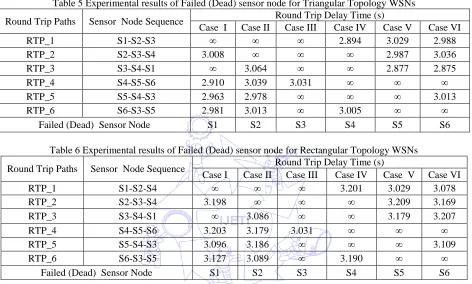
Table 5 Experimental results of Failed (Dead) sensor node for Triangular Topology WSNs

RTP_1 S1-S2-S3 ∞ ∞ ∞ 2.894 3.029 2.988

RTP_2 S2-S3-S4 3.008 ∞ ∞ ∞ 2.987 3.036

RTP_3 S3-S4-S1 ∞ 3.064 ∞ ∞ 2.877 2.875

RTP_4 S4-S5-S6 2.910 3.039 3.031 ∞ ∞ ∞

RTP_5 S5-S4-S3 2.963 2.978 ∞ ∞ ∞ 3.013

RTP_6 S6-S3-S5 2.981 3.013 ∞ 3.005 ∞ ∞

Failed (Dead) Sensor Node S1 S2 S3 S4 S5 S6

Table 6 Experimental results of Failed (Dead) sensor node for Rectangular Topology WSNs

RTP_1 S1-S2-S4 ∞ ∞ ∞ 3.201 3.029 3.078

RTP_2 S2-S3-S4 3.198 ∞ ∞ ∞ 3.209 3.169

RTP_3 S3-S4-S1 ∞ 3.086 ∞ ∞ 3.179 3.207

RTP_4 S4-S5-S6 3.203 3.179 3.031 ∞ ∞ ∞

RTP_5 S5-S4-S3 3.096 3.186 ∞ ∞ ∞ 3.109

RTP_6 S6-S3-S5 3.127 3.089 ∞ 3.190 ∞ ∞

Failed (Dead) Sensor Node S1 S2 S3 S4 S5 S6

Simulation results mentioned in above tables indicate the shift in monitoring task from one source node to other

automatically. It starts with S1 and S4 nodes which scan the entire network and then if fault is present, detection task is

transferred to S2 or S5. If fault is not detected here then task is shifted to S3 or S6. In this way detection task is shared between

different sensor nodes at different level or stages in WSNs thereby reducing the computational load on individual sensor node.

Fault tolerance is achieved by automatic rotation of from failed sensor node to the other non-faulty sensor node. Applicability of

this method is tested with the help of three topologies. Proper selection of path for RTPs in these topologies is utmost important

to achieve the desired results with less computation.

3.3 Detection of Malfunctioning Sensor Node

Now experiment is performed by adding a delay to any one sensor node (i.e. it behaves as malfunctioning sensor node) in

WSNs. For experimental purpose a delay of 5 s is added to a sensor node. Network is simulated in real time to measure the RTD

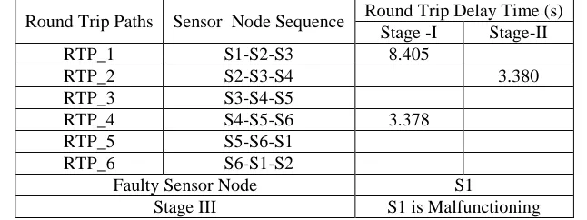
times of essential linear RTPs. Malfunctioning sensor node detection in three stages is elaborated in Table 7 with the help of

experimental results. Delay of 5 s is added to S1 sensor node. In first stage of examination RTP_1 and 4 are measured. Here it

was found that RTD time of the RTP_1 is higher and RTP_4 has less value than the threshold value. This result proves that S4,

(9)

value. As RTP_2 consists of S2, S3 and S4 sensor nodes, none of them are faulty. Above two stage results confirms the failure of

S1 node. Since RTD times are not infinity in any both stage concludes the malfunctioning of S1 sensor node.

Table 7 Three stage analysis of Malfunctioning sensor node in Circular topology of WSNs

Round Trip Paths Sensor Node Sequence Round Trip Delay Time (s) Stage -I Stage-II

RTP_1 S1-S2-S3 8.405

RTP_2 S2-S3-S4 3.380

RTP_3 S3-S4-S5

RTP_4 S4-S5-S6 3.378

RTP_5 S5-S6-S1

RTP_6 S6-S1-S2

Faulty Sensor Node S1

Stage III S1 is Malfunctioning

Six different cases are considered to verify the above test procedure circular, triangular and rectangular topologies. These

topologies are simulated to measure the RTD time of linear RTPs for six cases whose results are listed in Tables VIII, IX and X

respectively. In case I, S1 node is made to malfunction by adding delay of 5s. As a result of this RTD time of RTPs becomes

higher than the threshold value to which S1 belongs. Remaining RTPs has RTD time less than the threshold value. Now

observing the RTPs with higher RTD time indicates that S1 sensor is common to them. Higher RTD time of these RTPs confirms

that sensor node S1 is malfunctioning. Similar procedure of fault detection is used in remaining cases whose conclusions are

mentioned in the Tables VIII, IX and X respectively.

Table 8 Experimental results of Malfunctioning sensor node for Circular Topology WSNs

RTP_1 S1-S2-S3 8.405 8.379 8.388 3.383 3.378 3.378

RTP_2 S2-S3-S4 3.380 8.390 8.403 8.386 3.369 3.369

RTP_3 S3-S4-S5 3.369 3.375 8.376 8.379 8.386 3.375

RTP_4 S4-S5-S6 3.378 3.382 3.374 8.381 8.379 8.402

RTP_5 S5-S6-S1 8.397 3.390 3.369 3.379 8.381 8.389

RTP_6 S6-S1-S2 8.388 8.378 3.372 3.385 3.377 8.376

Malfunctioning Sensor node S1 S2 S3 S4 S5 S6

Table 9 Experimental results of Malfunctioning sensor node for Triangular Topology WSNs

RTP_1 S1-S2-S4 8.019 8.058 8.107 2.904 3.008 2.988

RTP_2 S2-S3-S4 3.008 7.819 8.037 7.789 2.763 3.036

RTP_3 S3-S4-S1 7.964 3.042 7.786 8.201 3.075 2.875

RTP_4 S4-S5-S6 2.909 3.035 3.031 8.005 8.057 7.877

RTP_5 S5-S4-S3 3.092 2.878 7.952 7.608 7.878 3.018

RTP_6 S6-S3-S5 2.905 2.989 7.833 3.103 7.797 7.905

(10)

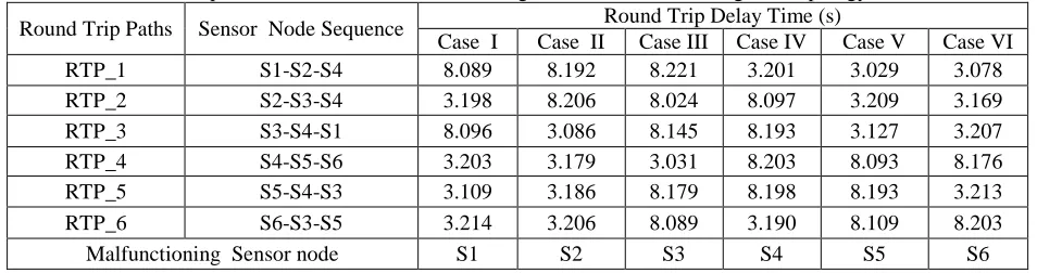
Table 10 Experimental results of Malfunctioning sensor node for Rectangular Topology WSNs

RTP_1 S1-S2-S4 8.089 8.192 8.221 3.201 3.029 3.078

RTP_2 S2-S3-S4 3.198 8.206 8.024 8.097 3.209 3.169

RTP_3 S3-S4-S1 8.096 3.086 8.145 8.193 3.127 3.207

RTP_4 S4-S5-S6 3.203 3.179 3.031 8.203 8.093 8.176

RTP_5 S5-S4-S3 3.109 3.186 8.179 8.198 8.193 3.213

RTP_6 S6-S3-S5 3.214 3.206 8.089 3.190 8.109 8.203

Malfunctioning Sensor node S1 S2 S3 S4 S5 S6

From the simulation results mentioned in above tables it is observed that the fault monitoring task is shifted from one source

node to other automatically. Initially it starts with S1 and S4 nodes which scan the entire network and then if fault is present,

detection task is either transferred to S2 or S5. Here if fault is not detected then this task is shifted to S3 or S6. In this way

detection task is shared between different sensor nodes at different level or stages in WSNs thereby reducing the computational

load on individual sensor node. Automatic rotation of source node provides the fault tolerance by shifting the detection task from

failed sensor node to the other non-faulty sensor node. Applicability of this method is tested with the help of three topologies.

Proper selection of path for RTPs in these topologies is utmost important to achieve the desired results with less computation.

3.4 Energy Utilized during RTD Time Measurement

Implemented wireless sensor node works on 3.3 v battery. Sensor node draws the current of 42.5 mA for the period of 354

ms during transmission and the current of 42.9 mA for period of 360 ms during reception. Sensor node is utilized in only three

RTPs during fault detection. It is acting as source node in one RTP and intermediate node for remaining two RTPs. Hence it is

transmitting and receiving the signal or packet for three times each during fault detection.

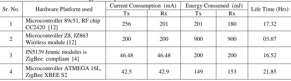
In Table 11 energy consumed by sensor node during transmission and reception is presented. Referring Table 11, total

energy consumed by sensor node during fault detection process is 302mJ. Energy consumption and lifetime of wireless sensor

nodes designed by using different hardware platforms is mentioned in Table 12. All the wireless sensor nodes designed using

different hardware platform are considered to be powered by a uniform battery with 3.3v and 2000mAh. The battery energy is

obtained as follows

EBAT = 3.3 V x 2000 mAh = 6.6 J/h (1)

Then the lifetime of sensor node is calculated with the help of following formula

LifetimeSENSOR = EBAT / ESENSOR = (6.6J/h) / Sensor Energy (2)

Table 11 Energy consumption of sensor node during fault detections

Sensor Node Energy during Voltage (V) Current (mA) Time (ms) Energy (mJ)

Transmission 3.3 42.5 354*3=1062 149

Reception 3.3 42.9 360*3=1080 153

(11)

Table 12 Energy consumption and Lifetime of various wireless sensor nodes

Sr. No. Hardware Platform used Current Consumption (mA) Energy Consumed (mJ) Life Time (Hrs)

Tx Rx Tx Rx

1 Microcontroller 89c51, RF chip

CC2420 [12] 256 201 201 180 17.32

2 Microcontroller Z8, JZ863

Wireless module [12] 200 200 900 900 03.67

3 JN5139 Jennic modules is

ZigBee compliant [4] 46.48 46.48 200 200 16.52

4 Microcontroller ATMEGA 16L,

ZigBee XBEE S2 42.5 42.9 149 153 21.85

Referring to Table 12; the energy consumed by fourth (4) wireless sensor node is 25% less than other sensor nodes. Hence

lifetime of the designed wireless sensor node is 28.5% more than other nodes. This will improve the overall lifetime of WSNs

and thereby increasing the quality of service (QoS).

4. Conclusions

In this paper energy efficient fault tolerant scheme is presented to achieve fault detection effectively. Automatic rotation of

source node during detection process distributes the computational load amongst the sensor nodes of WSNs thereby saving the

energy. Further sensor energy requirement is curtailed by managing the optimal role of sensor node in the fault detection with the

help of linear RTPs. Utilization of proposed algorithm gives the satisfactory results for failed as well as malfunctioning sensor

node. Applicability of investigated method is verified with the help of triangular and rectangular topologies of WSNs. Energy

consumption of various sensor nodes used in WSNs are compared to prove the efficiency of proposed method. Still scope lies in

optimizing the energy by reducing the numbers of RTPs required in fault detection. This method is useful to detect the single

faulty sensor node in WSNs. Further work to detect the multiple faulty sensor nodes is in progress and will be communicated.

References

[1]D. Angelis, A. Moschitta, P. Händel, and P. Carbone, “Experimental radio indoor positioning systems based on round-trip time measurement,” Advances in Measurement Systems, pp. 195-219, April 2010.

[2]Boudhir, B. Mohamed, and B. A. Mohamed, “New technique of wireless sensor networks localization based on energy consumption,” International Journal of Computer Applications, vol. 9, no. 12, pp. 25-28, November 2010.

[3]R. Alena, R. Gilstrap, J. Baldwin, T. Stone, and P. Wilson, “Fault tolerance in ZigBee wireless sensor networks,” IEEEAC Paper #1480, Version I, pp. 1-15, December 2010.

[4]R. S. J. Reyes, J. C. Monje, and et al, “Implementation of Zigbee-based and ISM-based wireless sensor and actuator network with throughput, power and cost comparisons,” WSEAS Transactions on Communications, vol. 9, no. 7, pp. 395-405, July 2010.

[5]A. Saeed, A. Stranieri, and R. Dazeley, “Fault-tolerant energy-efficient priority-based routing scheme for the multisink healthcare sensor networks,” International Scholarly Research Network ISRN Sensor Networks, pp. 1-11, 2012.

[6]Wint Yi Poe and Jens B. Schmitt, “Node deployment in large wireless sensor networks: coverage, energy consumption, and worst-case delay,” ACM(AINTEC’09), Bangkok, pp. 1-8, November 18–20, 2009.

[7]T. W. Pirinen, J. Yli-Hietanen, P. Pertil ¨a, and A. Visa, “Detection and compensation of sensor malfunction in time delay based direction of arrival,” IEEE Circuits and Systems, vol.4, pp. 872-875, May 2004.

[8]S. S. Ahuja, R. Srinivasan, and M. Krunz, “Single-Link failure detection in all-optical networks using monitoring cycles and paths,” The IEEE/ACM Transactions on Networking, vol. 17, no. 4, pp. 1080-1093, August 2009.

(12)

[10]M. Zahid Khan, M. Merabti, B. Askwith, and F. Bouhafs, “A fault-tolerant network management architecture for wireless sensor networks,” PG Net, pp. 1-6, 2010.

[11]R. N. Duche and N. P. Sarwade, “Sensor node failure detection based on round trip delay and paths in WSNs,” IEEE Sensor Journal, vol. 14, no. 2, pp. 455-464, February 2014.

[12]K. Shinghal, A. Noor, N. Srivastava, and R. Singh, “Power measurements of wireless sensor networks node,” International Journal of Computer Engineering & Science, vol. 1, no. 1, pp. 8-13, May 2011.

[13]R. N. Duche and N. P. Sarwade, “Round trip delay time as a linear function of distance between the sensor nodes in wireless sensor network,” IJESET, vol. 1, no. 2, pp. 20-26, February 2012.

[14]L. Paradis and Q. Han, “A survey of fault management in wireless sensor networks,” Springer Journal of Network and Systems Management, vol.15, no.2, pp. 171-190, June 2007.

[15]G. Vennira Selvi and R. Manoharan, “Cluster based fault identification and detection algorithm for WSN- A survey,” International Journal of Computer Trends and Technology (IJCTT), vol. 4, no. 10, pp. 3491-3496, October 2013.

[16]S. Zeadally, N. Jabeur, and I. M. Khan, “Hop-based approach for holes and boundary detection in wireless sensor networks,”IET Wireless Sensor Systems, vol. 2, no. 4, pp. 328–337, 2012.

[17]N. Jamal, A. Karaki, R. U. Mustafa, and A. E. Kamal, “Data aggregation and routing in wireless sensor networks: optimal

and heuristic algorithms,” The ACM International Journal of Computer and Telecommunication Networking, vol. 53, no. 7, pp. 945-960, May 2009.

[18]M. Collotta and G. Pau, “Bluetooth for Internet of things: A fuzzy approach to improve power management in smart homes,” Computers & Electrical Engineering, vol. 44, pp. 137-152, May 2015.