Choice of
V
for
V
-Fold Cross-Validation in Least-Squares
Density Estimation
Sylvain Arlot [email protected]
Laboratoire de Math´ematiques d’Orsay
Univ. Paris-Sud, CNRS, Universit´e Paris-Saclay 91405 Orsay, France
Matthieu Lerasle [email protected]
CNRS
Univ. Nice Sophia Antipolis LJAD CNRS UMR 7351 06100 Nice France
Editor:Xiaotong Shen
Abstract
This paper studies V-fold cross-validation for model selection in least-squares density es-timation. The goal is to provide theoretical grounds for choosingV in order to minimize the least-squares loss of the selected estimator. We first prove a non-asymptotic oracle inequality forV-fold cross-validation and its bias-corrected version (V-fold penalization). In particular, this result implies thatV-fold penalization is asymptotically optimal in the nonparametric case. Then, we compute the variance ofV-fold cross-validation and related criteria, as well as the variance of key quantities for model selection performance. We show that these variances depend on V like 1 + 4/(V −1), at least in some particular cases, suggesting that the performance increases much from V = 2 to V = 5 or 10, and then is almost constant. Overall, this can explain the common advice to take V = 5 —at least in our setting and when the computational power is limited—, as supported by some simulation experiments. An oracle inequality and exact formulas for the variance are also proved for Monte-Carlo cross-validation, also known as repeated cross-validation, where the parameterV is replaced by the numberB of random splits of the data.
Keywords: V-fold cross-validation, Monte-Carlo cross-validation, leave-one-out, leave-p -out, resampling penalties, density estimation, model selection, penalization
1. Introduction
Cross-validation methods are widely used in machine learning and statistics, for estimating the risk of a given statistical estimator (Stone, 1974; Allen, 1974; Geisser, 1975) and for selecting among a family of estimators. For instance, cross-validation can be used for model selection, where a collection of linear spaces is given (the models) and the problem is to choose the best least-squares estimator over one of these models. Cross-validation is also often used for choosing hyperparameters of a given learning algorithm. We refer to Arlot and Celisse (2010) for more references about cross-validation for model selection.
it is unique, which is the goal of BIC for instance; see the survey by Arlot and Celisse (2010) for more details about this distinction. These two goals cannot be attained simultaneously in general (Yang, 2005).
We assume throughout the paper that the goal of model selection is estimation. We refer to Yang (2006, 2007) and Celisse (2014) for some results and references on cross-validation methods with an identification goal.
Then, a natural question arises: which cross-validation method should be used for min-imizing the risk of the final estimator? For instance, a popular family of cross-validation methods isV-fold cross-validation (Geisser, 1975, often calledk-fold cross-validation), which depends on an integer parameter V, and enjoys a smaller computational cost than other classical cross-validation methods. The question becomes (1) whichV is optimal, and (2) can we do almost as well as the optimal V with a small computational cost, that is, a small V? Answering the second question is particularly useful for practical applications where the computational power is limited.
Surprisingly, few theoretical results exist for answering these two questions, especially with a non-asymptotic point of view (Arlot and Celisse, 2010). In short, it is proved in least-squares regression that at first order, V-fold cross-validation is suboptimal for model selection (with an estimation goal) if V stays bounded, because V-fold cross-validation is biased (Arlot, 2008). When correcting for the bias (Burman, 1989; Arlot, 2008), we recover asymptotic optimality whateverV, but without any theoretical result distinguishing among values ofV in second order terms in the risk bounds (Arlot, 2008).
Intuitively, if there is no bias, increasingV should reduce the variance of theV-fold cross-validation estimator of the risk, hence reduce the risk of the final estimator, as supported by some simulation experiments (Arlot, 2008, for instance). But variance computations for unbiased V-fold methods have only been made in the asymptotic framework for a fixed estimator, and they focus on risk estimation instead of model selection (Burman, 1989).
This paper aims at providing theoretical grounds for the choice of V by two means: a non-asymptotic oracle inequality valid for any V (Section 3) and exact variance computa-tions shedding light on the influence of V on the variance (Section 5). In particular, we would like to understand why the common advice in the literature is to take V = 5 or 10, based on simulation experiments (Breiman and Spector, 1992; Hastie et al., 2009, for instance).
The results of the paper are proved in the least-squares density estimation framework, because we can then benefit from explicit closed-form formulas and simplifications for theV -fold criteria. In particular, we show thatV-fold cross-validation and all leave-p-out methods are particular cases of V-fold penalties in least-squares density estimation (Lemma 1).
The first main contribution of the paper (Theorem 5) is an oracle inequality with leading constant 1 +εn, withεn→0 as n→ ∞for unbiased V-fold methods, which holds for any
value of V. To the best of our knowledge, Theorem 5 is the first non-asymptotic oracle inequality for V-fold methods enjoying such properties: the leading constant 1 +εn is new
in density estimation, and the fact that it holds whatever the value of V had never been obtained in any framework. Theorem 5 relies on a new concentration inequality for the
Theorem 5 may not imply the asymptotic optimality of V-fold penalization. Let us also emphasize that the leading constant is 1 +εnwhateverV for unbiasedV-fold methods, with εn independent from V in Theorem 5. So, second-order terms must be taken into account
for understanding how the model selection performance depends onV. Section 4 proposes a heuristic for comparing these second order terms thanks to variance comparisons. This motivates our next result.
The second main contribution of the paper (Theorem 6) is the first non-asymptotic variance computation forV-fold criteria that allows to understand precisely how themodel selection performance of V-fold cross-validation or penalization depends on V. Previous results only focused on the variance of the V-fold criterion (Burman, 1989; Bengio and Grandvalet, 2005; Celisse, 2008, 2014; Celisse and Robin, 2008), which is not sufficient for our purpose, as explained in Section 4. In our setting, we can explain, partly from theoretical results, partly from a heuristic argument, why taking, say, V > 10 is not necessary for getting a performance close to the optimum, as supported by experiments on synthetic data in Section 6.
An oracle inequality and exact formulas for the variance are also proved for other cross-validation methods: Monte-Carlo cross-cross-validation, also known as repeated cross-cross-validation, where the parameter V is replaced by the number B of random splits of the data (Sec-tion 8.1), and hold-out penaliza(Sec-tion (Sec(Sec-tion 8.2).
Notation. For any integerk>1,JkKdenotes{1, . . . , k}. For any vectorξ
JnK := (ξ1, . . . , ξn) and anyB ⊂JnK,ξB denotes (ξi)i∈B,|B|denotes the
cardinality of B and Bc=
JnK\B.
For any real numbers t, u, we definet∨u:= max{t, u},u+:=u∨0 andu−:= (−u)∨0. All asymptotic results and notation o(·) orO(·) are for the regime when the numbern
of observations tends to infinity.
2. Least-Squares Density Estimation and Definition of V-Fold Procedures
This section introduces the framework of the paper, the main procedures studied, and some useful notation.
2.1 General Statistical Framework
Let ξ, ξ1, ..., ξn be independent random variables taking value in a Polish space X, with
common distributionP and densityswith respect to some known measureµ. Suppose that
s∈L∞(µ), which implies thats∈L2(µ). The goal is to estimatesfromξ
JnK= (ξ1, . . . , ξn),
that is, to build an estimator bs=bs(ξ
JnK)∈L
2(µ) such that its lossk
b
s−sk2 is as small as possible, where for anyt∈L2(µ),ktk2 :=R
Xt2dµ.
Projection estimators are among the most classical estimators in this framework (see, for example, DeVore and Lorentz, 1993 and Massart, 2007). Given a separable linear subspace
Sm of L2(µ) (called a model), the projection estimator ofsonto Sm is defined by b
sm := argmin t∈Sm
ktk2−2P
n(t) , (1)
where Pn is the empirical measure; for any t∈L2(µ),Pn(t) = R
tdPn= n1Pni=1t(ξi). The
denoted by
Pnγ(t) =ktk2−2Pn(t) where ∀x∈ X,∀t∈L2(µ), γ(t;x) =ktk2−2t(x) .
The functionγ is called the least-squares contrast. Note thatSm ⊂L1(P) sinces∈L2(µ).
2.2 Model Selection
When a finite collection of models (Sm)m∈Mn is given, following Massart (2007), we want
to choose from data one among the corresponding projection estimators (bsm)m∈Mn. The
goal is to design a model selection procedure mb : Xn 7→ M
n so that the final estimator
e
s := bsmb has a quadratic loss as small as possible, that is, comparable to the oracle loss infm∈Mnksbm −sk
2. This goal is what is called the estimation goal in the Introduction. More precisely, we aim at proving that an oracle inequality of the form
kbs
b
m−sk2 6Cn inf
m∈Mn
ksbm−sk2 +Rn
holds with a large probability. The procedure mb is called asymptotically optimal whenRn
is much smaller than the oracle loss and Cn → 1, as n → +∞. In order to avoid trivial
cases, we will always assume that|Mn|>2.
In this paper, we focus on model selection procedures of the form
b
m:= argmin
m∈Mn
crit(m) ,
where crit : Mn 7→ R is some data-driven criterion. Since our goal is to satisfy an oracle inequality, an ideal criterion is
critid(m) =kbsm−sk
2− ksk2 =−2P(
b
sm) +ksbmk
2 =P γ(
b sm) .
Penalization is a popular way of designing a model selection criterion (Barron et al., 1999; Massart, 2007)
crit(m) =Pnγ(bsm) + pen(m)
for some penalty function pen : Mn → R, possibly data-driven. From the ideal criterion
critid, we get the ideal penalty
penid(m) := critid(m)−Pnγ(bsm) = (P −Pn)γ(bsm) = 2(Pn−P)(bsm) (2)
= 2(Pn−P)(bsm−sm) + 2(Pn−P)(sm) = 2kbsm−smk
2+ 2(P
n−P)(sm) ,
where sm:= argmin t∈Sm
P γ(t) = argmin
t∈Sm
kt−sk2
is the orthogonal projection of s onto Sm in L2(µ). Let us finally recall some useful and
classical reformulations of the main term in the ideal penalty (2), that proves in particular the last equality in Eq. (2): If Bm = {t ∈ Sm s.t. ktk 6 1} and (ψλ)λ∈Λm denotes an
orthonormal basis of Sm inL2(µ), then
(Pn−P)(sbm−sm) = X
λ∈Λm
(Pn−P)(ψλ) 2
=kbsm−smk2 = sup t∈Bm
(Pn−P)(t) 2
,
(3)
2.3 V-Fold Cross-Validation
A standard approach for model selection is cross-validation. We refer the reader to Arlot and Celisse (2010) for references and a complete survey on cross-validation for model selection. This section only provides the minimal definitions and notation necessary for the remainder of the paper.
For any subset A⊂JnK, let
Pn(A):= 1 |A|
X
i∈A
δξi and sb
(A)
m := argmin t∈Sm
n
ktk2−2Pn(A)(t)
o .
The main idea of cross-validation is data splitting: someT ⊂JnKis chosen, one first trains
b
sm(·) with ξT, then test the trained estimator on the remaining data ξTc. The hold-out
criterion is the estimator of critid(m) obtained with this principle, that is, critHO(m, T) :=Pn(Tc)γ
b s(mT)
=−2Pn(Tc)
b s(mT)
+ b s(mT)
2
, (4)
and all cross-validation criteria are defined as averages of hold-out criteria with various subsets T.
Let V ∈ {2, . . . , n} be a positive integer and let B = B
JVK = (B1, . . . ,BV) be some
partition of JnK. TheV-fold cross-validation criterion is defined by
critVFCV(m,B) := 1
V V X
K=1
critHO(m,BcK) .
Compared to the hold-out, one expects cross-validation to be less variable thanks to the averaging overV splits of the sample intoξBK and ξBcK.
Since critVFCV(m,B) is known to be a biased estimator ofE[critid(m)], Burman (1989) proposed the bias-corrected V-fold cross-validation criterion
critcorr,VFCV(m,B) := critVFCV(m,B) +Pnγ(bsm)−
1
V V X
K=1
Pnγ
b s(BcK)
m
.
In the particular case whereV =n, this criterion is studied by Massart (2007, Section 7.2.1, p. 204–205) under the name cross-validation estimator.
2.4 Resampling-Based and V-Fold Penalties
Another approach for building general data-driven model selection criteria is penalization with a resampling-based estimator of the expectation of the ideal penalty, as proposed by Efron (1983) with the bootstrap and later generalized to all resampling schemes (Arlot, 2009). LetW ∼ W be some random vector ofRn independent fromξJnK with
1
n n X
i=1
and denote by PnW = n−1Pn
i=1Wiδξi the weighted empirical distribution of the sample.
Then, the resampling-based penalty associated with W is defined as
penW(m) :=CWEW h
Pn−PnW
γ sbmWi
, (5)
where bsmW ∈argmint∈Sm{PnWγ(t)}, EW[·] denotes the expectation with respect to W only
(that is, conditionally to the sampleξ
JnK), and CW is some positive constant.
Resampling-based penalties have been studied recently in the least-squares density estimation framework (Lerasle, 2012), assuming that W is exchangeable, that is, its distribution is invariant by any permutation of its coordinates.
Since computing exactly penW(m) has a large computational cost in general for ex-changeableW, some non-exchangeable resampling schemes were introduced by Arlot (2008), inspired byV-fold cross-validation: given some partition B=B
JVKofJnK, the weight vector W is defined by Wi= (1−Card(BJ)/n)−11i /∈BJ for some random variableJ with uniform
distribution overJVK. Then,PnW =P(B c J)
n so that the associated resampling penalty, called V-fold penalty, is defined by
penVF(m,B, x) := x
V V X
K=1
Pn−P
(Bc K)
n
γbs(BcK)
m
= 2x
V V X
K=1
P(B
c K)
n −Pn
b s(B
c K)
m
(6)
wherex >0 is left free for flexibility, which is quite useful according to Lemma 1 below.
2.5 Links Between V-Fold Penalties, Resampling Penalties and (Corrected)
V-Fold Cross-Validation
In this paper, we focus our study on V-fold penalties because Lemma 1 below shows that formula (6) covers all V-fold and resampling-based procedures mentioned in Sections 2.3 and 2.4.
First, when V = n, the only possible partition is BLOO = {{1}, . . . ,{n}}, and the
V-fold penalty is called the leave-one-out penalty penLOO(m, x) := penVF(m,BLOO, x). The associated weight vector W is exchangeable, hence Eq. (6) leads to all exchangeable resampling penalties since they are all equal up to a deterministic multiplicative factor in the least-squares density estimation framework when Pn
i=1Wi = n, as proved by Lerasle (2012).
For V-fold methods, let us assumeB is a regular partition of JnK, that is,
V =|B|>2 divides n and ∀K ∈JVK, |BK|= n
V . (Reg)
Then, we get the following connection between V-fold penalization and cross-validation methods.
Lemma 1 For least-squares density estimation with projection estimators, under assump-tion (Reg),
critVFCV(m,B) =Pnγ(bsm) + penVF
m,B, V −1 2
(8)
critLPO(m, p) =Pnγ(bsm) + penLPO
m, p,n p −
1 2
(9)
=Pnγ(bsm) + penLOO
m,(n−1)n/p−1/2
n/p−1
(10)
=Pnγ(bsm) + penVF
m,BLOO,(n−1)n/p−1/2
n/p−1
where for any p∈Jn−1K, the leave-p-out cross-validation criterion is defined by
critLPO(m, p) := 1 |Ep|
X
A∈Ep Pn(A)γ
b s(mAc)
with Ep :=
A⊂JnK s.t. |A|=p
and the leave-p-out penalty is defined by
∀x >0, penLPO(m, p, x) := x |Ep|
X
A∈Ep
Pn−P(A
c)
n
γ
b s(mAc)
.
Lemma 1 is proved in Section A.1.
Remark 2 Eq. (7) was first proved by Arlot (2008) in a general framework that includes least-squares density estimation, assuming only (Reg). Eq.(10)follows from Lerasle (2012, Lemma A.11) sincepenLPO belongs to the family of exchangeable resampling penalties, with weights Wi := (1−p/n)−11i /∈A and A is randomly chosen uniformly over Ep; note that Pn
i=1Wi = n for these weights. It can also be deduced from Proposition 3.1 by Celisse
(2014), see Section A.1.
Remark 3 It is worth mentioning here the cross-validation estimators studied by Massart (2007, Chapter 7). First, the unbiased cross-validation criterion defined by Rudemo (1982) is exactly critcorr,VFCV(m,BLOO) (see also Massart, 2007, Section 7.2.1). Second, the
pe-nalized estimator of Massart (2007, Theorem 7.6) is the estimator selected by the penalty
penLOO m,(1 +)
6(n−1)2 2
n−(1 +)6 !
for some >0 such that (1 +)6< n (see Section A.1 for details).
So, in the least-squares density estimation framework and assuming only (Reg), Lemma 1 shows that it is sufficient to studyV-fold penalization with a free multiplicative factorxin front of the penalty for studying alsoV-fold cross-validation (x=V−1/2), correctedV-fold cross-validation (x=V −1), the leave-p-out (V =nand x= (n−1)(n/p−1/2)/(n/p−1)) and all exchangeable resampling penalties. For anyC >0 andBsome partition ofJnKinto
V pieces, takingx=C(V −1), theV-fold penalization criterion is denoted by
C(C,B)(m) :=Pnγ(bsm) + penVF m,B, C(V −1)
A key quantity in our results is the bias E[C(C,B)(m) −critid(m)]. From Lemma 13 in Section A.2, we have
EpenVF(m,B, V −1)
=Epenid(m)
= 2Ekbsm−smk
2
, (12)
so that for anyC >0,
EC(C,B)(m)−critid(m)
= 2(C−1)Eksbm−smk
2
. (13)
In Sections 3–7, we focus our study onV-fold methods, that is, we study the performance of the V-fold penalized estimatorssb
b
m, defined by
b
m=mb C(C,B)
= argmin
m∈Mn
C(C,B)(m) , (14)
for all values ofV and C >1/2. Additional results on hold-out (penalization) are given in Section 8.2 to complete the picture.
3. Oracle Inequalities
In this section, we state our first main result, that is, a non-asymptotic oracle inequality satisfied by V-fold procedures. This result holds for any divisor V >2 of n, any constant
x=C(V −1) in front of the penalty withC >1/2, and provides an asymptotically optimal oracle inequality for the selected estimator when C → 1 (assuming the setting is non parametric). In addition, as proved by Section 2.5, it implies oracle inequalities satisfied by leave-p-out procedures for allp.
3.1 Concentration of V-Fold Penalties
Concentration is the key property to establish oracle inequalities. Let us start with some new concentration results forV-fold penalties.
Proposition 4 Let ξ
JnK be i.i.d. real-valued random variables with density s ∈ L
∞(µ),
B some partition of JnK into V pieces satisfying (Reg), Sm a separable linear space of
measurable functions and (ψλ)λ∈Λm an orthonormal basis ofSm. Define
Bm =
t∈Sm s.t. ktk61 Ψm = X
λ∈Λm
ψ2λ= sup
t∈Bm
t2 bm:=k p
Ψmk∞
Dm:=P(Ψm)− ksmk2 =nE
h
ksm−sbmk
2i , where bsm is defined by Eq.(1), and for any x, >0,
ρ1(m, , s, x, n) :=
ksk∞x
n +
b2m+ksk2 x2 3n2 .
Then, an absolute constantκexists such that for anyx>0, with probability at least1−8e−x, for any∈(0,1], the following two inequalities hold true
penVF(m,B, V −1)−2Dm
n
6
Dm
n +κρ1(m, , s, x, n) (15)
penVF(m,B, V −1)−2ksm−bsmk
2
6
Dm
Proposition 4 is proved in Section A.2. Eq. (15) gives the concentration of the V-fold penalty around its expectation 2Dm/n = E[penid(m)], see Eq. (12). Eq. (16) gives the concentration of theV-fold penalty around the ideal penalty, see Eq. (2). Optimizing over
, the first order of the deviations of penVF(m,B, V −1) around penid(m) is driven by √
Dm/n. The deviation term in Proposition 4 does not depend on V and cannot therefore
help to discriminate between different values of this parameter.
3.2 Example: Histogram Models
Histograms on R provide some classical examples of collections of models. Let X be a measurable subset of R, µ denote the Lebesgue measure on X and m be some countable partition ofX such thatµ(λ)>0 for anyλ∈m. The histogram spaceSmbased onmis the
linear span of the functions (ψλ)λ∈Λmwhere Λm =mand for everyλ∈m,ψλ=µ(λ)
−1/21
λ.
More precisely, we illustrate our results with the following examples.
Example 1 (Regular histograms on X =R)
Mn=
mh, h∈JnK where ∀h∈JnK, mh=
λ h,
λ+ 1
h
, λ∈Z
.
In Example 1, definingdmh=hfor everyh∈JnK, for everym∈ Mn,Dm =dm−ksmk
2since Ψm is constant and equal todm. Therefore, Proposition 4 shows that penVF(m,B, V −1) is asymptotically equivalent to pendim(m) := 2dm/nwhen dm → ∞. Penalties of the form
of pendim are classical and have been studied for instance by Barron et al. (1999).
Example 2 (k-rupture points on X = [0,1])
Mn=nmh
Jk+1K,xJkK
s.t. x1<· · ·< xk∈Jn−1Kand∀i∈Jk+ 1K, hi∈Jxi−xi−1K
o ,
where x0 = 0, xk+1 =n and for any x1, . . . , xk ∈Jn−1K such that x1 <· · · < xk and any
h
Jk+1K∈N
k+1, m
h
Jk+1K,xJkK
is defined as the union
[
i∈JkK
xi−1
n +
(xi−xi−1)(λ−1) nhi
,xi−1 n +
(xi−xi−1)λ nhi
, λ∈JhiK
.
In other words,mh
Jk+1K,xJkK
splits [0,1]into k+ 1pieces (at thexi), and then splits the i-th
piece into hi pieces of equal size.
In Example 2, the function Ψm is constant on each interval [xi−1, xi), equal tohi, therefore,
Dm=
k+1
X
i=1
hiP ξ ∈[xi−1, xi)
− ksmk2 .
3.3 Oracle Inequality for V-Fold Procedures
• A uniform bound on theL∞ norm of the L2 ball of the models
∀m∈ Mn, bm 6
√
n (H1)
where we recall thatbm := supt∈Bmktk∞ and Bm:={t∈Sm,ktk61}.
• The family of the projections ofs is uniformly bounded.
∃a >0, ∀m∈ Mn, ksmk∞6a , (H2)
• The collection of models is nested.
∀(m, m0)∈ M2n, Sm∪Sm0 ∈ {Sm, Sm0} (H20)
Hereafter, we defineA:=a∨ ksk∞when (H2) holds andA:=ksk∞when (H20) holds. On histogram spaces, (H1) holds if and only if infm∈Mninfλ∈mµ(λ) > n
−1, and (H2) holds
witha=ksk∞.
Theorem 5 Letξ
JnK be i.i.d. real-valued random variables with common densitys∈L
∞(µ),
B some partition of JnK into V pieces satisfying (Reg) and (Sm)m∈Mn be a collection of
separable linear spaces satisfying (H1). Assume that either (H2) or (H20) holds true. Let
C∈(1/2,2], δ:= 2(C−1) and, for any x, >0,
ρ2(, s, x, n) :=
Ax n +
1 +ksk 2
n
x2
3n and xn=x+ log|Mn| . For every m∈ Mn, let bsm be the estimator defined by Eq. (1) andse=bsmb where
b
m=mb C(C,B)
is defined by Eq. (14). Then, an absolute constant κ exists such that, for any x > 0, with probability at least 1−e−x, for any∈(0,1],
1−δ−− 1 +δ++
kes−sk26 inf
m∈Mn
kbsm−sk2+κρ2(, s, xn, n) . (17)
Theorem 5 is proved in Section A.3.
Taking >0 small enough in Eq. (17), Theorem 5 proves that V-fold model selection procedures satisfy an oracle inequality with large probability. The remainder term can be bounded under the following classical hypothesis
∃a0 >0,∀n∈N?, |Mn|6na
0
. (H3)
For instance, (H3) holds in Example 1 with a0 = 1 and in Example 2 with a0 =k. Under (H3), the remainder term in Eq. (17) is bounded by L(logn)2/(3n) for someL >0, which is much smaller than the oracle loss in the nonparametric case.
The leading constant in the oracle inequality (17) is (1 +δ+)/(1−δ−) + o(1) by choosing
δ= 2(C−1) is the amount of bias of theV-fold penalization criterion, as shown by Eq. (13). Given this interpretation of δ, the model selection literature suggests that no asymptotic optimality result can be obtained in general whenδ 6= o(1) in the nonparametric case (see, for instance, Shao, 1997). Therefore, even if the leading constant (1 +δ+)/(1−δ−) is only an upper bound, we conjecture that it cannot be taken as small as 1 + o(1) unlessδ= o(1); such a result can be proved in our setting using similar arguments and assumptions as the ones of Arlot (2008) for instance.
For bias-corrected V-fold cross-validation, that is, C = 1 hence δ = 0, Theorem 5 shows a first-order optimal non-asymptotic oracle inequality, since the leading constant (1 +)/(1−) can be taken equal to 1 + o(1), and the remainder term is small enough in the nonparametric case, under assumption (H3), for instance. Such a result valid with no upper bound onV had never been obtained before in any setting.
V-fold cross-validation is also analyzed by Theorem 5, since by Lemma 1 it corresponds to C = 1 + 1/(2(V −1)), hence δ = 1/(V −1). When V is fixed, the oracle inequality is asymptotically sub-optimal, which is consistent with the result proved in regression by Arlot (2008). On the contrary, if B =Bn hasVn blocs, with Vn→ ∞, Theorem 5 implies under
assumption (H3) the asymptotic optimality ofVn-fold cross-validation in the nonparametric
case.
The bound obtained in Theorem 5 can be integrated and we get
1−δ−− 1 +δ++E
h
kes−sk2i6E
h
inf
m∈Mn
kbsm−sk2 i
+κ0ρ2
, s,log |Mn|
for some absolute constant κ0 >0.
AssumingC >1/2 is necessary, according to minimal penalty results proved by Lerasle (2012). Assuming C 6 2 only simplifies the presentation; ifC > 2, the same proof shows that Theorem 5 holds withκ replaced by Cκ.
An oracle inequality similar to Theorem 5 holds in a more general setting, as proved in a previous version of this paper (Arlot and Lerasle, 2012, Theorem 1); we state a less general result here for simplifying the exposition, since it does not change the message of the paper. First, assumption (Reg) can be relaxed into assuming the partition B is close to regular, that is,
Bis a partition of JnK of size V and sup
k∈JVK
Card(Bk)− n V
61 , (Reg
0)
which can hold for any V ∈ JnK. Second, data ξ1, . . . , ξn can belong to a general Polish
space X, at the price of some additional technical assumption.
3.4 Comparison with Previous Works on V-Fold Procedures
Few non-asymptotic oracle inequalities have been proved for V-fold penalization or cross-validation procedures.
Theorem 5 considers the strongest possible oracle, that is, trained with n data. Optimal oracle inequalities were proved by Celisse (2014) for leave-p-out estimators with p n, a case also treated in Theorem 5 by takingV =nand C = (n/p−1/2)/(n/p−1) as shown by Lemma 1. Ifpn,C∼1, henceδ = o(1) and we recover the result of Celisse (2014).
Concerning V-fold penalization, previous results were either valid for V =n only—by Massart (2007, Theorem 7.6) and Lerasle (2012) for least-squares density estimation, by Arlot (2009) for regressogram estimators—, or forV bounded whenntends to infinity—by Arlot (2008) for regressogram estimators. In comparison, Theorem 5 provides a result valid for all V, except for the assumption that V divides n, which can be removed (Arlot and Lerasle, 2012). In particular, the loss bound by Arlot (2008) deteriorates when V grows, while it remains stable in our result. Our result is therefore much closer to the typical behavior of the loss ratiokes−sk2/inf
m∈Mnkbsm−sk
2 ofV-fold penalization, which usually decreases as a function of V in simulation experiments, see Section 6 and the experiments by Arlot (2008), for instance.
Theorem 5 may not satisfactorily address the parametric setting, that is, when the collection (Sm)m∈Mn contains some fixed true model. In such a case, the usual way to
obtain asymptotic optimality is to use a model selection procedure targetting identification, that is, taking C →+∞ when n→ +∞. For instance, Celisse (2014, Theorem 3.3) shows that log(n)Cnis a sufficient condition for such a result.
4. How to Compare Theoretically the Performances of Model Selection Procedures for Estimation?
The main goal of the paper is to compare the model selection performances of several (V -fold) cross-validation methods, when the goal is estimation, that is, minimizing the loss kbs
b
m−sk2 of the final estimator. In this section, we discuss how such a comparison can be
made on theoretical grounds, in a general setting.
For some data-driven function C:Mn→R, the goal is to understand howksb
b
m(C)−sk2
depends onC when the selected model is
b
m(C)∈argmin
m∈Mn
C(m) . (18)
From now on, in this section, C is assumed to be a cross-validation estimator of the risk, but the heuristic developed here applies to the general case.
Ideal comparison. Ideally, for proving thatC1is a better method thanC2in some setting, we would like to prove that
bs
b
m(C1)−s
2
<(1−εn) sb
b
m(C2)−s
2
(19)
with a large probability, for some εn>0.
Previous works and their limits. When the goal is estimation, the classical way to analyze the performance of a model selection procedure is to prove an oracle inequality, that is, toupper bound (with a large probability or in expectation)
bs
b
m(C)−s
2
− inf
m∈Mn
n
kbsm−sk2 o
or Rn(C) := bs
b
m(C)−s
2 infm∈Mn
Alternatively, asymptotic results show that whenntends to infinity,Rn(C)→1 (asymptotic optimality of C) or Rn(C1) ∼ Rn(C2) (asymptotic equivalence of C1 and C2); see Arlot and Celisse (2010, Section 6) for a review of such results. Nevertheless, proving Eq. (19) requires a lower bound on Rn(C) (asymptotic or not), which has been done only once for some cross-validation method, to the best of our knowledge. In some least-squares regression setting, V-fold cross-validation (CVF) performs (asymptotically) worse than all asymptotically optimal model selection procedures sinceRn(CVF)>κ(V)>1 with a large probability (Arlot, 2008).
The major limitation of all these previous results is that they can only compare C1 toC2 at first order, that is, according to limn→∞Rn(C1)/Rn(C2), which only depends on the bias ofCi(m) (i= 1,2) as an estimator ofE[kbsm−sk
2], hence, on the asymptotic ratio between the training set size and the sample size (Arlot and Celisse, 2010, Section 6). For instance, the leave-p-out and the hold-out with a training set of size (n−p) cannot be distinguished at first order, while the leave-p-out performs much better in practice, certainly because its “variance” is much smaller.
Beyond first-order. So, we must go beyond the first-order of Rn(C) and take into ac-count the variance of C(m). Nevertheless, proving a lower bound on Rn(C) is already
challenging at first order—probably the reason why only one has been proved up to now, in a specific setting only—so the challenge of computing a precise lower bound on the second order term ofRn(C) seems too high for the present paper. We propose instead a heuristic showing that the variances of some quantities—depending on (Ci)i=1,2 and onMn—can be
used as a proxy to a proper comparison of Rn(C1) and Rn(C2) at second order. Since we focus on second-order terms, from now on, we assume that C1 and C2 have the same bias, that is,
∀m∈ Mn, EC1(m)
=EC2(m)
. (SameBias)
In least-squares density estimation, given Lemma 1, this means that for i∈ {1,2},
Ci =C(C,B
i)
as defined by Eq. (11), with different partitions Bi satisfying (Reg) with differentV =Vi,
but the same constantC >0;C= 1 corresponds to the unbiased case.
The variance of the cross-validation criteria is not the correct quantity to look at. If we were only comparing cross-validation methods C1,C2 as estimators of Ekbsm−sk
2
for every single m ∈ Mn, we could naturally compare them through their mean squared errors. Under assumption (SameBias), this would mean to compare their variances. This can be done from Eq. (23) below, but it is not sufficient to solve our problem, since it is known that the best cross-validation estimator of the risk does not necessarily yield the best model selection procedure (Breiman and Spector, 1992). More precisely, the selected model mb(C) defined by Eq. (18) is unchanged when C(m) is translated by any random quantity, but such a translation does change Var(C(m)) and can make it as large as desired. For model selection, what really matters is that
sign C(m1)− C(m2)= sign
kbsm1−sk 2− k
b
as often as possible for every (m1, m2) ∈ M2n, and that most mistakes in the ranking of
models occur when kbsm1 −sk 2− k
b
sm2−sk
2 is small, so that k
b s
b
m(C)−sk2 cannot be much larger than infm∈Mn{kbsm−sk
2}.
Heuristic. The heuristic we propose goes as follows. For simplicity, we assume that
m? = argminm∈MnE[kbsm−sk
2] is uniquely defined. If the goal was identification, we could directly state that for anyC, the smaller is P(m=mb(C)) for all m6=m
?, the better should
be the performance of mb(C). In this paper, our goal is estimation, but a similar claim can be conjectured by considering “allm∈ Mn sufficiently far fromm? in terms of risk”, that
is, all m ∈ Mn such that E[kbsm−sk
2] is significantly worse than
E[kbsm?−sk
2]. Indeed, for any m “close tom?” in terms of risk, selecting m instead of m? does not significantly change the performance ofmb(C); on the contrary, for anym “far fromm
?” in terms of risk,
selectingm instead ofm? does increase significantly the risk E[ksbmb(C)−sk 2].
Then, our idea is to find a proxy for P(m = mb(C)), that is, a quantity that should
behave similarly as a function ofC and its “variance” properties. For all m, m0 ∈ Mn, let
∆C(m, m0) :=C(m)− C(m0),N some standard Gaussian random variable and, for allt∈R, Φ(t) =P(N > t). Then, for every m∈ Mn
P mb(C) =m
=P ∀m0 6=m,∆C(m, m0)<0 min
m06=mP ∆C(m, m
0)<0
(20)
≈ min
m06=mP
E∆C(m, m0)+N
p
Var(∆C(m, m0))<0 (21)
= Φ SNRC(m)
where SNRC(m) := max
m06=m
E∆C(m, m0)
q
Var ∆C(m, m0)
.
So, if SNRC1(m)>SNRC2(m) for allm“sufficiently far fromm
?”,C
1 should be better than C2. Assuming (SameBias) holds true and that
{m?}= argmin
m∈Mn
EC1(m)
= argmin
m∈Mn
EC2(m)
, (SameMin)
this leads to the following heuristic
∀m6=m0, Var ∆C1(m, m 0)
<Var ∆C2(m, m 0)
⇒ C1 better than C2 . (22) Indeed, for everym6=m0, assumption (SameMin) implies that SNRCi(m)>0 fori= 1,2,
hence we can restrict the max in the definition of SNRCi to allm
0 such that
E[∆Ci(m, m
0)]
is positive. By assumption (SameBias), the numerator in the definition of SNRCi does not
depend on i, hence the ratio is maximal when the denominator is minimal, which leads to Eq. (22). Let us make some remarks.
• The quantity ∆C(m, m0) appears in relative bounds (Catoni, 2007, Section 1.4) which can be used as a tool for model selection (Audibert, 2004).
• Assumptions (SameBias) and (SameMin) hold true in particular in the unbiased case, that is, whenE[Ci(m)] =E[kbsm−sk
2] for all m∈ M
• Assumption (SameMin) is necessary: Figure 3 shows an example where a larger variance corresponds to better performance under assumption (SameBias) alone.
• As noticed above, the heuristic (22) should apply when the goal is estimation and when the goal is identification, provided that (SameBias) and (SameMin) hold true. What should depend on the goal is the suitable amount of bias forCi(m) as an
estimator of the riskE[kbsm−sk
2].
• Approximation (20) is the strongest one. Clearly, inequality6holds true. The equal-ity case occurs is for a very particular dependence setting, that is, when one among the events ({∆C(m, m0) <0}), m0 ∈ Mn, is included into all the others. In general,
the left-hand side is significantly smaller than the right-hand side; we conjecture that they vary similarly as a function of C.
• The Gaussian approximation (21) for ∆C(m, m0) does not hold exactly, but it seems reasonable to make it, at first order at least.
• The validity of approximations (20) and (21) is supported by the numerical experi-ments of Section 6.
In the heuristic (22), all (m, m0) do not matter equally for explaining a quantitative differ-ence in the performances of C. First, we can fix m0 = m?, since intuitively, the strongest candidate against any m 6=m? is m?, which clearly holds in all our experiments, see Fig-ures 18 and 24 in Section G of the Online Appendix. Second, as mentioned above, if m
and m? are very close, that is, k b
sm−sk2/kbsm?−sk
2 is smaller than the minimal order of magnitude we can expect for Rn(C) with a data-drivenC, takingm instead ofm? does not
decrease the performance significantly. Third, if Φ(SNRC(m)) is very small, increasing it even by an order of magnitude will not affect the performance ofmb(C) significantly; hence, all m such that, say, SNRC(m) (log(n))α for all α >0, can also be discarded. Overall, pairs (m, m0) that really matter in (22) are pairs (m, m?) that are at a “moderate distance”, in terms ofE[kbsm−sk
2− k
b
sm?−sk2].
5. Dependence on V of V-Fold Penalization and Cross-Validation
Let us now come back to the least-squares density estimation setting. Our goal is to compare the performance of cross-validation methods having the same bias, that is, according to Section 2.5,mb(C(C,B)) with the same constantCbut different partitionsB, wheremb(C(C,B)) is defined by Eq. (14).
Theorem 6 Let ξ
JnK be i.i.d. random variables with common density s∈ L
∞(µ), B some
partition ofJnKintoV pieces satisfying (Reg), and(ψλ)λ∈Λm1,(ψλ)λ∈Λm2 two orthonormal
families in L2(µ). For any m, m0 ∈ {m1, m2}, we define Sm the linear span of (ψλ)λ∈Λm, sm the orthogonal projection ofsonto Sm in L2(µ), Ψm := supt∈Sms.t. ktk61t
2,
β m, m0:= X
λ∈Λm
X
λ0∈Λ m0
E
h
ψλ(ξ1)−P ψλ
ψλ0(ξ1)−P ψλ0
i2
Then, for every C >0,
Var C(C,B)(m1)= 2
n2
1 + 4C 2
V −1−
(2C−1)2
n
β(m1, m1) (23) + 4
nVar
1 +2C−1
n
sm1(ξ1)−
2C−1
2n Ψm1(ξ1)
and Var C(C,B)(m1)− C(C,B)(m2)
= 2
n2
1 + 4C 2
V −1 −
(2C−1)2
n
B(m1, m2) (24) + 4
nVar
1 +2C−1
n
(sm1−sm2)(ξ1)−
2C−1
2n (Ψm1 −Ψm2)(ξ1)
where C(C,B) is defined by Eq.(11). Theorem 6 is proved in Section A.4.
Unbiased case. WhenC = 1, Theorem 6 shows that
Var C(1,B)(m1)− C(1,B)(m2)
=a+
1 + 4
V −1− 1
n
b
for some a, b > 0 depending on n, m1, m2 but not on V. If we admit that the heuristic (22) holds true, this implies that the model selection performance of bias-corrected V-fold cross-validation improves when V increases, but the improvement is at most in a second order term as soon asV is large. In particular, even ifab, the improvement fromV = 2 to 5 or 10 is much larger than fromV = 10 toV =n, which can justify the commonly used principle that takingV = 5 or V = 10 is large enough.
Assuming in addition that Sm1 and Sm2 are regular histogram models (Example 1 in Section 3.2) with dm1 that divides dm2, then, by Lemma 19 in Section B.2 of the Online Appendix,
a= 4
n
1 + 1
n 2
Var sm1(ξ)−sm2(ξ)
≈ O
1
nksm1−sm2k 2
and b= 2
n2B(m1, m2) ksm2k 2dm2
n2 . Whendm2/nis at least as large asksm1−sm2k
2, we obtain that the first-order term in the variance is of the form α+β/(V −1) where α, β > 0 do not depend on V and are of the same order of magnitude, as supported by the numerical experiments of Section 6. Then, increasingV from 2 tondoes reduce significantly the variance, by a constant multiplicative factor.
Let Cid(m) := Pnγ(bsm) +E[penid(m)] be the criterion we could use if we knew the
expectation of the ideal penalty. From Proposition 17 in Section B of the Online Appendix,
Var Cid(m1)− Cid(m2)
= 2
n2
1− 1
n
B(m1, m2) + 4
nVar
1− 1
n
(sm1−sm2)(ξ1) + 1
2n(Ψm1−Ψm2)(ξ1)
which easily compares to formula (24) obtained for the V-fold criterion when C = 1. Up to smaller order terms, the difference lies in the first term, where (1 + 4/(V −1)−1/n) is replaced by (1−1/n) when using the expectation of the ideal penalty instead of a V-fold penalty. In other words, the leave-one-out penalty—that is, taking V = n—behaves like the expectation of the ideal penalty.
We can also compare Eq. (23) with the asymptotic results obtained by Burman (1989), which imply that for any fixed modelm1
Var C(1,B)(m1)−P γ(bsm1)
= γ0
n +
V
V −1γ1+γ2
1
n2 + o
1
n2
with γ0, γ1, γ2 that depend on m1 and γ1 > 0. Here, putting C = 1 in Eq. (23) yields a result with a similar flavour, valid for all n>1, even if Eq. (23) computes the variance of a slightly different quantity.
Cross-validation criteria. V-fold cross-validation and the leave-p-out are also covered by Theorem 6, according to Lemma 1, respectively with C = 1 + 1/(2(V −1)) and with
V = n and C = 1 + 1/(2(n/p−1)). As in the unbiased case, increasing V decreases the variance, and if we admit that the heuristic (22) holds true,V-fold cross-validation performs almost as well as the leave-(n/V)-out as soon as V is larger than 5 or 10.
Similarly, the variances of the V-fold cross-validation and leave-p-out criteria, for in-stance, can be derived from Eq. (23). In the leave-p-out case, we recover formulas obtained by Celisse (2014) and Celisse and Robin (2008), with a different grouping of the variance components; Eq. (23) clearly emphasizes the influence of the bias—through (C−1)—on the variance. For V-fold cross-validation, we believe that Eq. (23) shows in a simpler way how the variance depends on V, compared to the result of Celisse and Robin (2008) which was focusing on the difference between V-fold cross-validation and the leave-(n/V)-out; here the difference can be written
8
n2
1
V −1 − 1
n−1
1 + 1 2(V −1)
2
β(m1, m1) .
A major novelty in Eq. (23) is also to cover a larger set of criteria, such as bias-corrected
V-fold cross-validation. Note that Var(C(C,B)(m1)) is generally much larger than Var C(C,B)(m1)− C(C,B)(m2)
,
which illustrates again why computing the former quantity might not help for understanding the model selection properties ofC(C,B), as explained in Section 4. For instance, comparing Eq. (23) and (24), changingsm1 intosm1−sm2 in the second term can reduce dramatically the variance whensm1 andsm2 are close, which happens for the pairs (m1, m2) that matter for model selection according to Section 4.
The variance of other criteria and their increments are computed in subsequent sections of the paper and in the Online Appendix: Monte-Carlo cross-validation (Theorem 10 in Section 8.1 and Theorem 24 in Section C.4) and hold-out penalization (Proposition 28 in Section D.2).
Remark 7 The term B(m1, m2) does not depend on the choice of particular bases of Sm1
and Sm2: as proved by Proposition 18 in Section B of the Online Appendix
B(m1, m2) =nVar (bsm1−bsm2)(ξ)
−(n+ 1) Var (sm1−sm2)(ξ)
0 0.1 0.2 0.3 0.4 0.5 0.6 0.7 0.8 0.9 1 0
0.2 0.4 0.6 0.8 1 1.2 1.4 1.6
0 0.1 0.2 0.3 0.4 0.5 0.6 0.7 0.8 0.9 1
0 0.5 1 1.5 2 2.5 3 3.5
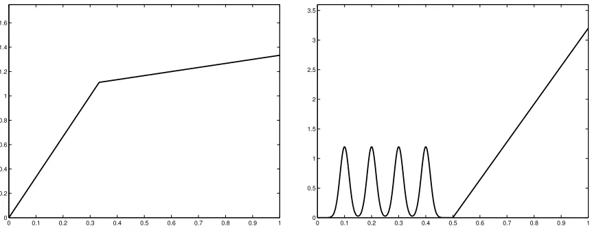
Figure 1: The two densities considered. Left: setting L. Right: setting S.
6. Simulation Study
This section illustrates the main theoretical results of the paper with some experiments on synthetic data.
6.1 Setting
In this section, we take X = [0,1] andµ is the Lebesgue measure onX. Two examples are considered for the target densitysand for the collection of models (Sm)m∈Mn.
Two density functions sare considered, see Figure 1:
• Setting L:s(x) = 103x106x<1/3+ (1 +x3)11>x>1/3.
• Setting S: s is the mixture of the piecewise linear density x 7→ (8x −4)11>x>1/2 (with weight 0.8) and four truncated Gaussian densities with means (k/10)k=1,...,4 and standard deviation 1/60 (each with weight 0.05).
Two collections of models are considered, both leading to histogram estimators: for everym∈ Mn,Sm is the set of piecewise constant functions on some partition Λm of X.
• “Regu” for regular histograms: Mn={1, . . . , n}where for everym∈ Mn, Λm is the
regular partition of [0,1] into m bins.
• “Dya2” for dyadic regular histograms with two bin sizes and a variable change-point:
Mn= [
k∈{1,...,en}
{k} ×n0, . . . ,log2(k)
o
×n0, . . . ,log2(en−k)
o
whereen=bn/log(n)c and for every (k, i, j)∈ Mn, Λ(k,i,j) is the union of the regular partition of [0, k/en) into 2
i pieces and the regular partition of [k/ e
n,1] into 2j pieces.
The difference between “Regu” and “Dya2” can be visualized on Figure 2, on which the corresponding oracle estimators bs
b
m? have been plotted for one sample in setting S, where
b
m? ∈argmin
m∈Mn
0 0.1 0.2 0.3 0.4 0.5 0.6 0.7 0.8 0.9 1 0
0.5 1 1.5 2 2.5 3 3.5
0 0.1 0.2 0.3 0.4 0.5 0.6 0.7 0.8 0.9 1
0 0.5 1 1.5 2 2.5 3 3.5
Figure 2: Oracle estimator for one sample of size n= 500, in setting S. Left: Regu. Right: Dya2.
Setting Oracle(Regu) Oracle(Dya2) Best(Regu) Best(Dya2)
L 13.4±0.1 5.46±0.02 25.8±0.1 19.4±0.1 S 62.4±0.1 43.9 ±0.1 100.9±0.2 83.4±0.2
Table 1: Comparison of Regu and Dya2: quadratic risksE[kbsmb−sk
2] of “Oracle” and “Best” estimators (multiplied by 103) with the two collections of models. “Best” means thatmb is the data-driven procedure minimizingE[kbsmb −sk
2] among all the data-driven procedures we considered in our experiments (see Section 6.2). “Oracle” means thatmb ∈argminm∈Mnkbsm−sk2 is the oracle model for each sample.
While “Regu” is one of the simplest and most classical collections for density estimation, the flexibility of “Dya2” allows to adapt to the variability of the smoothness of s. Intuitively, in settings L and S, the optimal bin size is smaller on [0,1/2] (where s is varying fastly) than on [1/2,1] (where |s0|is much smaller).
Another point of comparison of Regu and Dya2 is given by Table 1, that reports values of the quadratic risks obtained depending on the collection of models considered. Table 1 shows that in settings L and S, the collection Dya2 helps reducing the quadratic risk by approximately 20% (when comparing the best data-driven procedures of our experiment), and even more when comparing oracle estimators (30% in setting S, 59% in setting L). Therefore, in settings L and S, it is worth considering more complex collections of models (such as Dya2) than regular histograms.
two cases, the risk of the best data-driven procedure with Dya2 was larger than with Regu by 6 to 8%.
6.2 Procedures Compared
In each setting, we consider the following model selection procedures:
• pendim (Barron et al., 1999): penalization with pen(m) = 2 Card(Λm)/n.
• V-fold cross-validation withV ∈ {2,5,10, n}, see Section 2.3.
• V-fold penalties (with leading constant x = V −1, that is, bias-corrected V-fold cross-validation), forV ∈ {2,5,10, n}, see Section 2.4.
• for comparison, penalization with E[penid(m)], that is,mb(Cid).
Since it is often suggested to multiply the usual penalties by some factor larger than one (Arlot, 2008), we consider all penalties above multiplied by a factor C∈[0,10]. Complete results can be found in Section G of the Online Appendix.
6.3 Model Selection Performances
In each setting, all procedures are compared on N = 10 000 independent synthetic data sets of sizen= 500. For measuring their respective model selection performances, for each proceduremb(C) we estimate
Cor(C) :=ERn(C)
=E
" bs
b
m(C)−s
2 infm∈Mnksbm−sk
2
#
by the corresponding average over theN simulated data sets;Cor(C) represents the constant that would appear in front of an oracle inequality. The uncertainty of estimation ofCor(C) is measured by the empirical standard deviation of Rn(C) divided by
√
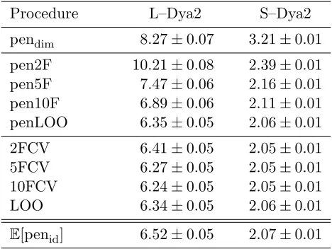
N. The results are reported in Table 2 for settings L and S, with the collection Dya2.
Results for Regu are not reported here since dimensionality-based penalties are already known to work well with Regu (Lerasle, 2012), so V-fold methods cannot improve signif-icantly their performance, with a larger computational cost. Complete results (including Regu, with n = 100 and n= 500) are given in Tables 3 and 4 in Section G of the Online Appendix, showing that the performances of pendim and V-fold methods indeed are very close.
Performance as a function of V. Let us first consider V-fold penalization. In both settings L and S, as suggested by our theoretical results, Cor decreases when V increases. The improvement is large whenV goes from 2 to 5 (27% for L, 10% for S) and small when
V goes from 5 to 10 and whenV goes from 10 ton= 500 (each time, 8% for L, 2% for S). Since the main influence of V is on the variance of the V-fold penalty, these experiments support our interpretation of Theorem 6 in Section 5: increasingV helps much more from 2 to 5 or 10 than from 10 to n.
Procedure L–Dya2 S–Dya2
pendim 8.27±0.07 3.21±0.01 pen2F 10.21±0.08 2.39±0.01 pen5F 7.47±0.06 2.16±0.01 pen10F 6.89±0.06 2.11±0.01 penLOO 6.35±0.05 2.06±0.01
2FCV 6.41±0.05 2.05±0.01 5FCV 6.27±0.05 2.05±0.01 10FCV 6.24±0.05 2.05±0.01 LOO 6.34±0.05 2.06±0.01
E[penid] 6.52±0.05 2.07±0.01
Table 2: Estimated model selection performances, see text. ‘LOO’ is a shortcut for ‘leave-one-out’, that is, V-fold withV =n= 500.
Indeed, increasingV simultaneously decreases the bias and the variance of theV-fold cross-validation criterion, leading to various possible behaviours of Cor as a function of V, de-pending on the setting. The same phenomenon has been observed in regression (Arlot, 2008).
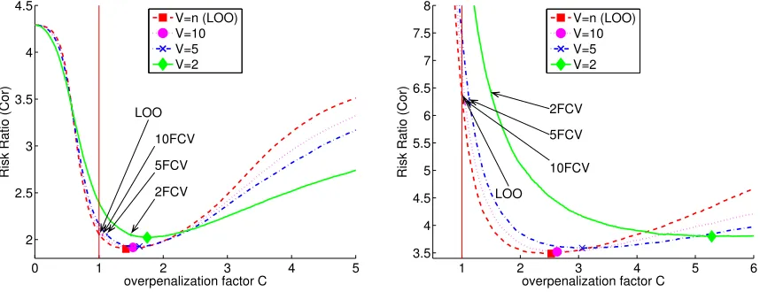
Overpenalization. In all settings considered in this paper, V-fold penalization performs much better when multiplying the penalty by C > 1, as illustrated by Figure 3. In par-ticular, the best overpenalization factor for penLOO is Cn? ≈2.5 for L-Dya2 and Cn? ≈1.4 for S-Dya2, when n= 500. Such a phenomenon, which can also be observed in regression (Arlot, 2008), is related to the fact that some nonparametric model selection problems are “practically parametric”, using the terminology of Liu and Yang (2011), that is, BIC beats AIC and the optimal C is closer to log(n)/2 than to 1. For instance, Figure 3 shows that L-Dya2 is practically parametric, while S-Dya2 is practically nonparametric since AIC beats BIC and the optimal C is close to 1.
Given an overpenalization factor C close to its optimal value Cn?, V-fold penalization performs significantly better than V-fold cross-validation in settings S-Dya2 and L-Dya2 (Figure 3). SinceV-fold cross-validation corresponds to taking
C=CVF(V) := 1 + 1 2(V −1)
0 1 2 3 4 5 2
2.5 3 3.5 4 4.5
Risk Ratio (Cor)
overpenalization factor C V=n (LOO) V=10 V=5 V=2
LOO
10FCV
5FCV
2FCV
1 2 3 4 5 6
3.5 4 4.5 5 5.5 6 6.5 7 7.5 8
Risk Ratio (Cor)
overpenalization factor C V=n (LOO) V=10 V=5 V=2
LOO
10FCV 5FCV 2FCV
Figure 3: Overpenalization in settings S-Dya2 (left) and L-Dya2 (right), with n = 500 in both cases. Each plot represents the estimated model selection performance
The results reported in Section G of the Online Appendix lead to similar conclusions in several other settings, as well as unshown results in a truly parametric setting, with a true model of dimension 2. Although a wider simulation study would be necessary to get general conclusions, this suggests at least that the heuristic of Section 4 and the theoretical results of Section 5 can be applied to both parametric and nonparametric settings.
Figure 3 also helps understanding how the performance of V-fold cross-validation de-pends onV in Table 2. Indeed, the performance ofV-fold cross-validation for each value of
V can be visualized on Figure 3 by taking the point of abscissa C=CVF(V) on the curve associated withV-fold penalization. Two phenomena are coupled when C 6Cn?, which al-ways holds in our simulations forV-fold cross-validation since maxV CVF(V) = 1.5 and the
estimated value of Cn? is always larger. (i) The performance improves when V is fixed and
C gets closer to Cn?. (ii) The performance improves whenC is fixed andV increases. Even if both phenomena (i) and (ii) seem quite universal, their coupling can result in various behaviours forV-fold cross-validation as a function ofV, as shown by Table 3 in Section G of the Online Appendix for instance.
Other comments.
• pendim performs much worse than V-fold penalization (except V = 2 in setting L) with the collection Dya2. On the contrary, pendim does well with Regu (see Table 3 in Section G of the Online Appendix), butV-fold penalization then performs as well.
• In other settings considered in a preliminary phase of our experiments, for V-fold penalization, differences between V = 2 and V = 5 were sometimes smaller or not significant, but always with the same ordering (that is, the worse performance for
V = 2 when C is fixed). In a few settings, for which the “change-point” in the smoothness of s was close to the median of sdµ, we found pendim among the best procedures with collection Dya2; then,V-fold penalization and cross-validation always had a performance very close to pendim. Both phenomena lead us to discard all settings for which there were no significant difference to comment.
6.4 Variance as a Function of V
We now illustrate the results of Section 5 about the variance of V-fold penalization and the heuristic of Section 4 about its influence on model selection. We focus on the unbiased case, that is, criteria C(1,B) with partitions B satisfying (Reg). Since the distribution of (C(1,B)(m))m∈Mn then only depends on V = |B|, we write CV instead of C(1,B) by abuse
of notation. All results presented in this subsection have been obtained from N = 10 000 independent samples in setting S with a sample size n= 100 and the collection Regu—for which models are naturally indexed by their dimension.
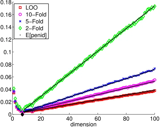
First, Figure 4 shows the variance of ∆CV(m, m
?) =C
V(m)− CV(m?) as a function of
the dimension m of Sm, illustrating the conclusions of Theorem 6: the variance decreases
when V increases. More precisely, the variance decrease is significant between V = 2 and
V = 5, an order of magnitude smaller betweenV = 5 andV = 10 and betweenV = 10 and
0 20 40 60 80 100 0
0.02 0.04 0.06 0.08 0.1 0.12 0.14 0.16 0.18
dimension LOO
10−Fold 5−Fold 2−Fold E[penid]
Cid. On Figure 4, we can remark that form > m?
Var(∆CV(m, m?))≈ 1
n2
K1
1 + K2
V −1
+K3
1 + K4
V −1
(m−m?)
with K1 ≈ 29, K2 ≈ 0.81, K3 ≈ 3.7 and K4 ≈ 3.8. The shape of the dependence on V already appears in Theorem 6, the above formula clarifies the relative importance of the terms calledaandbin Section 5, and their dependence on the dimensionmofSm. Remark
that the same behaviour holds when n = 500 with very close values for K3 and K4 (see Figure 25 in Section G of the Online Appendix), as well as in setting L with n = 100 or n = 500 with K3 ≈ 2.1 and K4 ≈ 4.2 (see Figures 19 and 30 in Section G of the Online Appendix). The fact that K4 is close to 4 in both settings supports that the term 1 + 4/(V −1) appearing Theorem 6 indeed drives how Var(∆CV(m, m?)) depends onV.
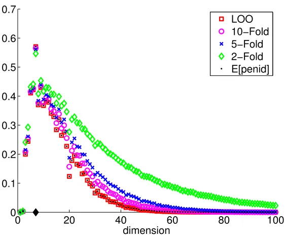
Figures 5 and 6 respectively show P(mb(C) =m) and its proxy Φ(SNRC(m)) as a
func-tion of m for C =CV with V ∈ {2,5,10, n} and for C = Cid. First, we remark that both quantities behave similarly as a function ofmandC—see also Figure 16 in Section G of the Online Appendix—supporting empirically the heuristic of Section 4. The decrease of the variance observed on Figure 4 whenV increases here translates into a better concentration of the distribution of mb(CV) around m?, which can explain the performance improvement observed in Section 6.3. Figures 5–6 actually show how the decrease of the variance quanti-tatively influences the distribution ofmb(CV): mb(C5) is significantly more concentrated than
b
m(C2), while the difference between V = 10 andV = 5 is much smaller and comparable to the difference between V =n and V = 10; Cn is hard to distinguish fromCid. Similar ex-periments withn= 500 and in setting L are reported in Section G of the Online Appendix, leading to similar conclusions.
7. Fast Algorithm for Computing V-Fold Penalties for Least-Squares Density Estimation
Since the use ofV-fold algorithms is motivated by computational reasons, it is important to discuss the actual computational cost ofV-fold penalization and cross-validation as a func-tion ofV. In the least-squares density estimation framework, two approaches are possible: a naive one—valid for all other frameworks—, and a faster one—specific to least-squares density estimation. For clarifying the exposition, we assume in this section that (Reg) holds true—so, V divides n. The general algorithm for computing the V-fold penalized criterion and/or theV-fold cross-validation criterion consists in training the estimator with data sets (ξi)i /∈Bj forj= 1, . . . , V and then testing each trained estimator on the data sets
(ξi)i∈Bj and/or (ξi)i /∈Bj. In the least-squares density estimation framework, for any model Sm given through an orthonormal family (ψλ)λ∈Λm of elements ofL
2(µ), we get the “naive” algorithm described and analysed more precisely in Section E.1 of the Online Appendix, whose complexity is of ordernV Card(Λm).
Several simplifications occur in the least-squares density estimation framework, that allow to avoid a significant part of the computations made in the naive algorithm.
Algorithm 1
Input: Bsome partition of {1, . . . , n}satisfying (Reg), ξ1, . . . , ξn∈ X and(ψλ)λ∈Λm
0 10 20 30 40 0
0.02 0.04 0.06 0.08 0.1 0.12 0.14 0.16
dimension
P(m is selected)
LOO 10−Fold 5−Fold 2−Fold E[penid]
Figure 5: P(mb(C) = m) as a function of m for five different C. Setting S-Regu, n = 100.
The black diamond showsm?= 7.
0 20 40 60 80 100
0 0.1 0.2 0.3 0.4 0.5 0.6 0.7
dimension
LOO 10−Fold 5−Fold 2−Fold E[penid]
1. For i∈ {1, . . . , V} and λ∈Λm, compute Ai,λ := VnPj∈Biψλ(ξj).
2. For i, j ∈ {1, . . . , V}, compute Ci,j :=Pλ∈ΛmAi,λAj,λ.
3. Compute S :=P
16i,j6V Ci,j and T := tr(C).
Output:
Empirical risk: Pnγ(sbm) =
−S
V2;
V-fold cross-validation criterion: critVFCV(m) = T
V(V −1)−
S − T (V −1)2;
V-fold penalty: penVF(m) = critVFCV(m)−Pnγ(bsm)
V −1/2 V −1 .
To the best of our knowledge, Algorithm 1 is new, even for computing the V-fold cross-validation criterion. Its correctness and complexity are analyzed with the following propo-sition.
Proposition 8 Algorithm 1 is correct and has a computational complexity of order
n+V2Card(Λm) .
In the histogram case, that is, whenΛm is a partition ofX and∀λ∈Λm,ψλ =µ(λ)−1/21λ,
the computational complexity of Algorithm 1 can be reduced to the order ofn+V2Card(Λm).
Proposition 8 is proved in Section E.2 of the Online Appendix. It shows that Algorithm 1 is significantly faster than the “naive” algorithm, by a factor of order
nV n+V2 =
1
V + V
n
−1
1 if 1V n .
Note that closed-form formulas are available for the leave-p-out criterion in least-squares density estimation (Celisse, 2014), allowing to compute it with a complexity of order
nCard(Λm) in general, and smaller in some particular cases—for instance,nfor histograms.
8. Discussion
Before discussing how to choose V when using V-fold methods for model selection—or more generally for choosing among a given family of estimators—, we state some additional results and we discuss the model selection literature in least-squares density estimation.
8.1 Monte-Carlo Cross-Validation
Our analysis ofV-fold procedures for model selection can be extended to some other cross-validation procedures. We here present results for Monte-Carlo cross-cross-validation (MCCV, Picard and Cook, 1984), also known as repeated cross-validation, whereB training samples of the same size n−pare chosen independently and uniformly (see also Arlot and Celisse, 2010, Section 4.3.2). Formally, we consider the criterion
critCV m,(TK)16K6B
:= 1
B B X
K=1
where T1, . . . , TB are subsets of JnK and we recall that the hold-out criterion is defined by
Eq. (4). We make the following three assumptions throughout this subsection
∃p∈Jn−1K, ∀j ∈JBK, |Tj|=n−p=nτn , (SameSize)
(TK)16K6B is independent from Dn , (Ind)
T1, . . . , TB are independent with uniform distribution over En−p , (MCCV)
where we recall thatEn−p ={A⊂JnK s.t.|A|=n−p}. Under these assumptions, we write
CMCCV(m) as a shortcut for crit
CV(m,(TK)16K6B).
Similarly to Theorem 5, we prove in Section C.3 of the Online Appendix the following oracle inequality for MCCV.
Theorem 9 Letξ
JnK be i.i.d. real-valued random variables with common densitys∈L
∞(µ),
(TK)16K6B some sequence of subsets of JnKsatisfying (SameSize), (Ind) and (MCCV)
and (Sm)m∈Mn be a collection of separable linear spaces satisfying (H1). Assume that
either (H2) or (H20) holds true. For every m ∈ Mn, let sbm be the estimator defined by
Eq.(1), and es=bs
b
m where
b
m∈argmin
m∈Mn
n
critCV m,(TK)16K6B o
and critCV is defined by Eq.(25). Let us define, for any x, y, >0,xn=x+ log|Mn|and
ρ3(, x, y, n, τn, B, A) :=
1
nτ2
n
1 +B∧(logn+y)
B(1−τn)
α
Ax τn
+(A∨1)x 2
3
withα= 1 under assumption (H2) andα= 2 under assumption (H20). Then, an absolute constant κ >0 exists such that, for anyx, y>0, with probability at least1−e−x−e−y, for any∈(0, κ−1),
1−
τn
kse−sk2 6 1 +
τn
inf
m∈Mn
n
kbsm−sk2 o
+κρ3(, xn, y, n, τn, B, A) . (26)
Theorem 9 actually is a corollary of a more general result (Theorem 23 in Section C.3 of the Online Appendix), which is valid without assumption (MCCV) and extends therefore our previous results onV-fold cross-validation).
Very few results exist in the literature about the model selection performance of MCCV with an estimation goal. Some asymptotic optimality result has been obtained by Burman (1990) for spline regression, and some oracle inequalities comparing the risk of the selected estimator with the risk of an oracle trained with τnn < n data have been proved by van
der Laan and Dudoit (2003) in a general framework and by van der Laan et al. (2004) for density estimation with the Kullback-Leibler loss. In comparison, Theorem 9 provides a precise non-asymptotic comparison to an oracle trained withndata.
As in Theorem 5, the leading constant of the oracle inequality (26) is directly related to the bias, which is here quantified byτn−1−1>0 instead ofδ. The remainder termρ3 is also comparable to ρ2 in Theorem 5: they differ by a factor betweenτn−2 (whenB is large
p=n/V in Theorem 9, hence τn= 1−V−1 ∈[1/2,1). Then, for the hold-out (B = 1),ρ3 is larger thanρ2 by a factorVα withα ∈ {1,2}. ForB =V, MCCV withτn= 1−V−1can
be called “Monte-Carlo V-fold” (MCVF); then, with y ≈logn, we loose a factor at most lognfor MCVF compared toV-fold cross-validation. Finally, whenB is large enough, that is, larger than V logn,ρ3 and ρ2 are of the same order.
The above comparison of remainder terms suggests a hierarchy between several cross-validation methods with a common training sample sizen−p=nτn: from the (presumably)
worse to the (presumably) best procedure, the hold-out, Monte-Carlo CV with B =V,V -fold CV, Monte-Carlo CV with B large and the leave-p-out. Nevertheless, upper bounds comparison can be misleading, so, following the heuristics (22) presented in Section 4, we compute below the variance of ∆C(m, m0) when C is a Monte-Carlo CV criterion.
Theorem 10 We consider the setting and notation of Theorem 6, and we assume that (SameSize), (MCCV) and (Ind) hold true. We recall that CMCCV(m) is defined above at the beginning of Section 8.1. Then, for regular histogram models m1, m2 (Example 1 in Section 3.2), we have
Var CMCCV(m1)− CMCCV(m2)
=C1MC(B, n, τn)
2
n2B(m1, m2) (27) +C2MC(B, n, τn)
4
nVar sm1(ξ1)−sm2(ξ1)
where
C1MC(B, n, τn) =
1
B
1
τ2
n
+ 2
τn(1−τn)
− 1
nτ3
n
+
1− 1
B "
1 + 1
n−1
1
τn
+ 1
2
− 1
nτ2
n #
C2MC(B, n, τn) =
1
B
1
n2τ3
n
+ 1
1−τn
+
1− 1
B
1 + 1
nτn 2
and we recall that τn=|TK|/n= 1−(p/n).
Theorem 10 is proved in Section C.4 of the Online Appendix, as a corollary of a more general result, called Theorem 24, which holds for all modelsm1, m2—not only regular histograms— and provides a formula for the variance of the criterion itself—not its increments. Let us make a few comments.
Eq. (27) is similar to the formula obtained for bias-corrected V-fold and V-fold penal-ization, see Eq. (24) in Theorem 6. In the particular case of regular histogram models, Eq. (24) even fits the general form of Eq. (27), with constants CipenVF(V, n, C) instead of
CiMC(B, n, τn).
Assuming the heuristics of Section 4 is valid, form1, m2which matter for model selection, the two terms 2n−2B(m1, m2) and 4n−1Var(sm1(ξ1)−sm2(ξ1)) are of the same order of magnitude (see Section 5). Then, we can compare model selection performance of several cross-validation methods by comparing the values of the constantsCi only.
In order to get a variance of the same order of magnitude as the one of bias-corrected
V-fold CV—that is, constantsCi of order 1—, MCCV requires to takeτn far enough from
![Table 1: Comparison of Regu and Dya2: quadratic risks E[∥s� �m−s∥2] of “Oracle” and “Best”estimators (multiplied by 103) with the two collections of models](https://thumb-us.123doks.com/thumbv2/123dok_us/9799369.1965864/19.612.94.522.90.257/table-comparison-quadratic-oracle-estimators-multiplied-collections-models.webp)