49
International Journal of Engineering and Management Research, Vol. 2, Issue-5, October 2012
ISSN No.: 2250-0758
Pages: 49-53
www.ijemr.net
Sensitivity Design for Arbitrary Order Plant with Time Delay
Using PI Controller
1
Gursewak Singh 1
Assistant Professor (ECE) , Yadawindra College Of Engineering ,Guru Kashi Campus, Punjabi University Patiala(Punjab)
1
Abstract- In present research, PI (propotional and integral) controller for sensitivity design with time delay under perturbed conditions is considered to achieve sensitivity stability criteria of arbitrary order plant . In particular, it has been shown that all PI gains that robustly stabilize a given uncertain (SISO) (LTI) system by keeping the sensitivty stability criterion . ⃦S(jω) ⃦
∞
⃒
=
∞<1 can be found by calculating the PID
controller gains Kp,Ki using frequency domain stability analysis presented in this paper developed on the preliminary knowledge of extended Hermite-Biehler Theorem.
Keywords- PI Controller,Time delay, Robust Stability, Frequency
domain,Sensitivity.
I. INTRODUCTION
In today technology ,because of immense application of PI controller in industry,Many engineer and scientist studied the Control system theory for stabilizing the system or plant and to determine the all set of PI controller gains Kp,Ki that meet certain design objective.Time delay in plant or system become a big problem which try to affect the performance of system and system get deviation from its accuracy. In the Single input and single output LTI plant example, PID controller gains are found that will guarantee robust and closed loop stability. S.P.Bhattacharey used a mathematical generalization of the Hermite-Biehler theorem to find all stabilizing PID controllers for systems with time-delay [1, 2, ,5].Recently, a large amount of research has been done on finding the set of all stabilizing arbitrary-order plant using frequency domain analysis as a result of this practical motivation[3,4,7].
For a given arbitrary-order LTI plant with variations of time delay , I proposed an algorithm to determine the all set of PI controllers gains which can be expressed as the first move for PI controller design for sensitivity criteria using
frequency domain analysis .Based on the result, this paper presents a design method in a systematic manner for S∞ PID controllers. The PI tuning methodology problem is first translated into simultaneous stabilization problem of a family of complex quasipolynomials and then the entire set of all PI gains KP and KI that can enable us to find the stability of these quasipolynomials. Robust stability creterian and nominal
stability criterion ⃒ <1 and some mathematical calucluation are discussed to achieve PID controller gains Kp and Ki in different planes (Kp, Ki) are elaborated. By tuning the two parameters gains kp,ki in the PI controller algorithm in section-V, the controller can provide control action designed for specific process requirements.The main advantages of this method ,It depends on frequency response which reduce complexity for achieving stability constraint. The response of the controller can be described in terms of the responsiveness of the controller to an error, the degree to which the controller overshoots the setpoint and the degree of system oscillation.
II. SENSITIVITY CONCEPT
1.Sensitivity [9]:
50
2.Robustness [8]:
Stability of LTI (SISO) linear time environment(Single Input and Single Output) under variation of uncertain parameter and environment conditions.A primary advantage of a closed-loop feedback control system is its ability to reduce the system ‘s sensitivity to parametric variations [8].
Figure 1 Plant G under effect of disturbance [8]
In Figure 1, r is desired force, d, n is disturbance and noise ,G is nominal plant , K is PI controller ,y is actual force.
Figure 2 :block diagram of sensitivity function [10]
In Figure 2 r is desired force ,G(s) is nominal plant , K(s) is PI controller ,y is actual force.
Where sensitivity S(s)= ………..………..1.1
C(s)=K(s) = PI controller consist of kp and ki gains can be written as follows
C(s)= K(s) = kp+ ……….1.2
G(s) is plant and system can be rewritten into real and imaginary part as follows
G(s) = ∂(s)+jσ(s) ………..1.3
where s→jω in frequency domain.
III. DEFINATIONS FOR CLOSED LOOP
Nominal stability (NS): system stable with no model uncertainty [8].
Nominal performance (NP): systems satisifies performance requirements with no model uncertainty [8].
Robust stability (RS): system stable for “all” perturbations ∆ [8].
Robust performance (RP): system satisifies performance requirements for “all” perturbations [8].
Now Criteria finally for magnitude of sensitivity S(s) must be less 1
. ⃦S(s) ⃦ <1 1.4
In figure 1.2,The SISO LTI plant with time delay can be described as
G(s) = ……….1.5
Gp(s) = G(s) * ……1.6
Put 1.5 into 1.6 obtain following equation.
Gp(s) = * …… …. 1.7
where 𝜏𝜏 is the time delay which varies as N(s) and D(s) are coprime polynomials in s, defined as
N(s)=Vm + Vm-1 +………+V1s+V0
D(s)= +Un-1 +………+ U1+U0
Here, V0, V1,Vm and U0, U1,Un-1 are real numbers, and n>m ,
C(s)= K(s) is PI controller written in following form.
C(s) =K(s)= Kp+ here s→ jω ,
Write PI controller as given below.
C(j𝜔𝜔)=K(jω)= Kp+ ………..1.8
The goal of the paper is to determine the set of (Kp, Ki) that satisfies the following S∞ performance index,From equation
1.1,Criteria ⃒ <1 for robust sensitivity constraint.
III. SENSITIVITY DESIGN METHODOLOGY
⃒ <1 Condition can be achieved using some mathematical equation for PI controller design with sensitivity criteria.
where
Gp(s) is nominal plant and S(s) is sensitivity
51
The sensitivity constraint equation 1.1 of the SISO system can be represented in its magnitude and phase as;
S(jω)=│S(jω)│e^(j∠S(jω)) OR <1 ∀ω …..1.9 Where θ= - ∠S(jω))
Lemma 1 consider that
G(s)= 1.10
is stable where R(s) , I(s) and E(s) are polynominals respectively with degree[R(s)] = ∝ ,degree [I(s)] =β, degree[E(s)]=∅ , ∝≤β ,∝≤∅, b,e and t are the highest order
coefficient of R(s) ,I(s) ,E(s) ,respectively. The Inequality . . ⃦G(jω) ⃦ <1 hols if and only if
1. . ⃦b ⃦>. ⃦t if ⃦ 𝛽𝛽>∅ , . ⃦e ⃦>. t ⃦ ⃦ if 𝛽𝛽<∅ or . ⃦b+e ⃦> . ⃦t ⃦ if 𝛽𝛽=∅
2. [ ]+ R(s) is stable for all θ in[0,2π]
Proof of lemma 1 is givem in [5] that is omitted here delebrately.
IV. VIEW FOR COMPLEX QUASIPOLYNOMIAL EQUATION AND THEOREM
Let us view the about Hermite –Biehler theorem [1]
Consider the quasipolynomial
φ(s) = 1.11
where ≠0 m and n is positive integers, is real or complex number ,and , ,……… are real numbers satisfying 0< < <……… . The term is the principle term.For stability of quasiupolynomial φ(s) in 1.11 equation ,the extended Hermite –Biehler theorem is explained as follows.
Theorem 1 [1].φ(s) in equation 1.11 is stable if and only if
1. (jω) and (jω)
2.
have onl real zeros and these zeros interlace;
(jω) (jω) - (jω) (jω) >0 for some ωϵ
(-∞,+∞).
Here , (jω) , (jω) (jω) , (jω) denotes the real and imaginary parts of φ(jω) and their first derivatives with respect to ω,respectively.
V. CONDITIONS FOR SENSITIVITY DESIGN
Step1 Determine nominal system is stable,f if yes move to step 2
Step 2 Find out kp and ki gains to find the stable sensitive region
Step 3 Put kp and ki in for loop for angle of 𝛉𝛉∈ [ 0, 2𝛑𝛑]
Step 4 Select Angle for obtaining intersection of lines of magenta colour .𝛉𝛉∈ [ 0, 2𝛑𝛑] in figure 3.
Step 5 Select Condition for sensitivity stability constraint given below, from equation 1.4 it must satisfy
<1 ……..1.12
Step 6 Find out stable and unstable region (intersections of lines)
Step 7 Check sensitivity stability constraint with PI controller using frequecy domain analysis.
Step 8 See figure 3,4,5
Now we will calculate the kp and ki gains with procedure given below.After calculating kp,ki gains , I will design two regions: Robust sensitive region and Unstable region.
Closed loop characterstic equation can be found putting equation 1.6 and 1.7 in equation 1.9 as in following mannner.
δ ( θ,s,kp,ki) =(s+(s*kp+ki)N(s) * )-s D(s)=0 or δ ( θ,s,kp,ki) ={s+(s*kp+ki)Gp(s)} -s =0 1.13
δ( θ,s,kp,ki)=0 must satisfy the sensitivity constraint for all
boundary of θϵ[0,2π] in kp and ki region.
Put Gp(s) nominal plant =∂+jσ ∂ is real part of plant and σ is imaginary part of plant , =cosθ+jsinθ and kp,ki is proportional and integral controller ,s→jω in 1.13 equation and break equation 1.13 into real and imaginary part.
jω+jω ∂ kp+∂ ki-ω σ kp+j σ ki – j ω cosθ+ωsinθ =0…..1.14
real part of 1.14 ∂ ki-ω σ kp+ωsinθ =0……….1.15
Imaginary part of 1.14 jω+jω ∂ kp+j σ ki – j ω cosθ=0…… ………..1.16
Find kp and ki ,apply matrix theory in above equation 1.15 nad 1.16 to find kp and ki.
kp=(∂*(cosθ-1)+(σ*sinθ))/( ) 1.1.7
ki=((σ*(cosθ-1)-(∂*sinθ))*ω)/( ) 1.18
VI. RESULTS AND CALCULATIONS
52 and communication delay in sytem τ is 0.1sec
Gp(s) = * ………1.20
Put 1.19 equation into 1.20 ,obtain following equation.
Gp(s) = * ………..1.21
-40 -30 -20 -10 0 10 20
-1200 -1000 -800 -600 -400 -200 0 200 Kp Ki
select Kp and Ki in (Kp,Ki) region using PI controller
Kp= 0.8525 Ki= 95.61
Kp = -1.221 Ki = -854.1 Unstable region sensitivity
stable region
Figure 3: sensitivity design in (Kp,Ki) region
In figure 3 ,I have plotted stable sensitive region(white) and unstable region (intersection of lines) in Kp,Ki region.
After plotting all PI controller regions with θϵ[0,2π],we will select Kp and Ki , PI controller gains to ensure sensitive stability.As per selected K1 and K2 PI controller in Kp,Ki regions ,we will check sensitivity stability criteria in figure 3 for K1 PI controller and in figure 4 for K2 Pi controller.
10-2 10-1 100 101 102
0 0.5 1 1.5 frequency M ag
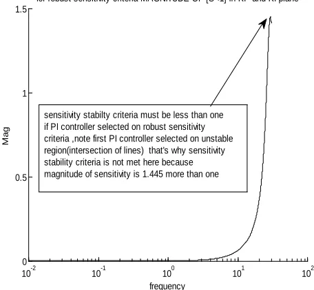
for robust sensitivity criteria MAGNITUDE OF [S<1] in KP and KI plane
sensitivity stabilty criteria must be less than one if PI controller selected on robust sensitivity criteria ,note first PI controller selected on unstable region(intersection of lines) that's why sensitivity stability criteria is not met here because magnitude of sensitivity is 1.445 more than one
Figure 4: sensitivity stablity with K1 PID controller in Kp,Ki region
From figure 4,It can be judged that sensitivity stability criteria can not be achieved,Becaude K1 PI controller selected on unstable region. see black colour line in figure 4 which reach upto 1.445 magnitude value in y-axis
10-2 10-1 100 101 102
0 0.1 0.2 0.3 0.4 0.5 0.6 0.7 0.8 0.9 frequency M ag
for robust sensitivity criteria MAGNITUDE OF [S<1] in KP and KI plane
sensitivity stability criteria in this case is 0.8685 that is less than one, this is our requirement for robust sensitivity stability criteria that we have achieved because PI controller selected in this case on white region which is only stable sensitive region.
Figure 5: sensitivity stablity with K2 PID controller in Kp,Ki region
From figure 5,It can be judged that sensitivity stability criteria can be achieved here ,Because K2 PI controller selected on stable sensitive region.see blue colour line in figure 5 which reach upto 0.8685 magnitude value in y-axis
Table 1.1
Sensitivity stability criteria with control of PI controller from figure 3
(kp,ki) Value on unstable region with K1 PI controller
. ⃦S(jω) ⃦ =⃒ <1 With K1 PI controller
Yes or NO
(kp,ki) values on stable sensitive region with K2 PI controller
. ⃦S(jω) ⃦
=⃒ <1 With K2 PI controller
Yes or No
(-1.221 , -854.1) From figure 3 NO ⃒ = 1.445
From figure 4
(0.8525 , 95.61) From figure 3 Yes ⃒ ⃒= 0.8685
From figure 5
VII. CONCLUSION
In this paper,I proposed a practical design method of S∞ PI
controller for general single input single output LTI(linera time invariant ) system with time delay.Note that I have shown the design problem to the S∞PI controller that has
53 region after plotting (Kp,Ki) region (heart type shape) shown
in figure 3.After selection of K1 PI controller on unstable region and K2 PI controller on stable sensitive region ,we achieved sensitive stability criteria with K1 PI controller shown in figure 4 and sensitive non-stability criteria with K2 PI controller shown in figure 5.With wide use of PID and PI controller in industrial process, It is expected that the all the result calculated in this paper will contribute to the development of practical control system design.
REFERENCES
[1] Ho., K.W., Datta, A., and S.P. Bhattacharya, “Generalizations of the Hermite-Biehler theorem,” Linear Algebra and its Applications, Vol. 302-303, 1999, pp. 135-153.
[2] Ho., K.W., Datta, A., and S.P. Bhattacharya, “,” Proc. 42nd IEEE Conf. on Decision and Control, Maui, Hawaii, 2003.
[3] Sujoldzic, S. and J.M. Watkins, “Stabilization of an arbitrary order transfer function with time delay using PI and PD controllers,” Proc. of American Control Conference, June 2006, pp. 2427-2432.
[4] Emami, T. and J.M. Watkins, “Robust performance characterization of PID controllers in the frequency domain,” WSEAS Transactions Journal of Systems and Control, Vol. 4, No. 5, May 2009, pp. 232-242.
[5] Bhattacharyya, S.P., Chapellat, H., and L.H. Keel, “Robust Control: The Parametric Approach”, Prentice Hall, N.J., 1995.
[6] Ho., K.W., Datta, A., and S.P. Bhattacharya, “PID stabilization of LTI plants with time-delay,” Proc. 42nd IEEE Conf. on Decision and Control, Maui, Hawaii, 2003.
[7] Bhattacharyya, S.P. and L.H. Keel, “PID controller synthesis free of analytical methods,” Proc. of IFAC 16th Triennial World Congress, Prague, Czech Republic, 2005.
[8] K. Zhou, J.C. Doyle, K. Glover, “Robust and Optimal Control”, Prentice-Hall,London, 1996.
[9] B.S Manke, .” linear control systems with matlab applications ,”Khana publishers,pp.202-203,2005.
[10] Linlin Ou,Peidong Zhou,weidong Zhang and Li Yu, “H∞ Robust Design of PID controller for Arbitrart order LTI system with time delay”,2011 50th IEEE conference on decision and control and Eueropean control conference
(CDC-ECC) orlando,FL,USA<December 12-15,2011.
![Figure 2 :block diagram of sensitivity function [10]](https://thumb-us.123doks.com/thumbv2/123dok_us/9789971.1964668/2.612.66.300.152.300/figure-block-diagram-sensitivity-function.webp)