A STATISTICAL METHOD FOR REGULARIZING NONLINEAR INVERSE PROBLEMS
by
Chad Clifton Hammerquist
A thesis
submitted in partial fulfillment of the requirements for the degree of
Master of Science in Mathematics Boise State University
© 2012
DEFENSE COMMITTEE AND FINAL READING APPROVALS
of the thesis submitted by
Chad Hammerquist
Thesis Title: A statistical method for regularizing nonlinear inverse problems Date of Final Oral Examination: 09 May 2012
The following individuals read and discussed the thesis submitted by student Chad Hammerquist, and they evaluated his presentation and response to questions dur-ing the final oral examination. They found that the student passed the final oral examination.
Jodi Mead, Ph.D. Chair, Supervisory Committee
Grady Wright, Ph.D, Member, Supervisory Committee Dr. Paul Micheals, Ph.D.,PE Member, Supervisory Committee
Inverse problems are typically ill-posed or ill-conditioned and require regulariza-tion. Tikhonov regularization is a popular approach and it requires an additional pa-rameter called the regularization papa-rameter that has to be estimated. Theχ2 method introduced by Mead in [8] uses theχ2distribution of the Tikhonov functional for linear inverse problems to estimate the regularization parameter. However, for nonlinear in-verse problems the distribution of the Tikhonov functional is not known. In this thesis, we extend the χ2 method to nonlinear problems through the use of Gauss Newton iterations and also with Levenberg Marquardt iterations. We derive approximate χ2
distributions for the quadratic functionals that arise in Gauss Newton and Levenberg Marquardt iterations. The approach is illustrated on two ill-posed nonlinear inverse problems: a nonlinear cross-well tomography problem and a subsurface electrical conductivity estimation problem. We numerically test the validity of assumptions in this approach by demonstrating that the theoreticalχ2 distributions agree closely with actual distributions. The nonlinearχ2 method is implemented in two algorithms, based on Gauss Newton and the Levenberg Marquardt methods, that dynamically estimate the regularization parameter using χ2 tests. We compare parameter esti-mates from the nonlinear χ2 method with estimates found using Occams inversion and the discrepancy principle on the cross-well tomography problem and on the subsurface electrical conductivity estimation problem. The χ2 method is shown to provide similar parameter estimates to estimates found using the discrepancy principle and is computationally less expensive. In addition, the χ2 method provided much better parameter estimates than Occams Inversion.
ABSTRACT . . . iii
LIST OF TABLES . . . vi
LIST OF FIGURES . . . vii
1 INTRODUCTION . . . 1
1.1 Inverse Problems . . . 1
1.1.1 Formulation of the Problem . . . 1
1.2 Ill-Posed Problems . . . 3
2 LEAST SQUARES . . . 6
2.1 Ordinary Least Squares (OLS) . . . 6
2.2 Nonlinear Least Squares . . . 7
2.2.1 Gauss-Newton Method and Levenberg-Marquardt . . . 9
2.3 Generalized Least Squares . . . 12
3 REGULARIZATION AND THE χ2 METHOD . . . 16
3.1 Choice of Regularization Parameter . . . 17
3.1.1 Nonlinear Regularization . . . 17
3.1.2 Statistical Framework . . . 18
3.1.3 Linear χ2 Method . . . 20
3.3 Nonlinearχ Method . . . 29
3.3.1 Numerical Implementation of Algorithms . . . 32
4 APPLICATION, SOLUTIONS, AND NUMERICAL EXPERIMENTS 34 4.1 Nonlinear Cross-Well Tomography . . . 35
4.1.1 Numerical Experiments . . . 36
4.1.2 Inversion Results . . . 38
4.2 Subsurface Electrical Conductivity Estimation . . . 42
4.2.1 Numerical Experiments . . . 43
4.2.2 Inversion Results . . . 44
5 CONCLUSIONS AND FUTURE WORK . . . 48
A ADDITIONAL THEOREMS . . . 52
4.1 Comparison of discrepancy principle toχ2 method on the cross-well to-mography problem,µ=mean(||xM−xtrue||/||xtrue||),σ =sqrt(var(||xM−
xtrue||/||xtrue||)) . . . 41 4.2 Comparison of theχ2 method to Occam’s inversion for the estimation
of subsurface conductivities, µ = mean(||xM −xtrue||/||xtrue||), σ =
sqrt(var(||xM−xtrue||/||xtrue||)) . . . 47
1.1 Contours of kd−F(x)k2
2 for two linear inverse problems. Left: Well-posed problem. Right: Ill-Well-posed problem. . . 4
4.1 The setup of the cross-well tomography problem. (Left) Shown here is the true velocity model(m/s). (Right) The ray paths crossing through region of interest (background is faded to make the ray paths more clear). . . 35 4.2 Histograms of Jek(xk+1). (Left): Jek with L = I, (Right): Jek with
L=4e. The mean of the sample is shown as the middle tick, and χ264
probability density function is shown as the solid blue line. . . 38 4.3 Solutions found for the tomography problem with L = 4e (Left)
So-lution found using the discrepancy principle. (Right) SoSo-lution found with Algorithm 1. . . 40 4.4 Solutions found for the tomography problem when L = I. (Left)
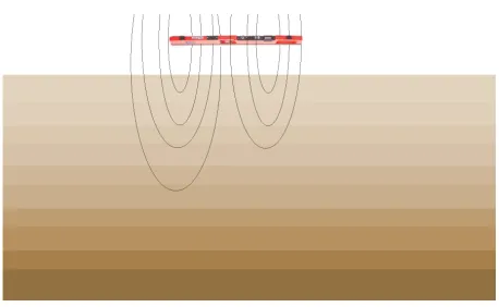
Solution found using the discrepancy principle. (Right) Solution found with Algorithm 1. . . 40 4.5 A representation of the soil-conductivity estimation. The instrument
depicted in the top of image represents a ground conductivity meter creating a time-varying electromagnetic field in the layered earth beneath. 42
e
D . The mean of the sample is shown as the middle tick, and the
χ218, χ216 density functions are shown as the solid blue line. . . 44 4.7 (Left) The unregularized solution. (Right) The solution found with
Occam’s inversion. . . 46 4.8 The parameters found using the χ2 method. (Left) L =
e
D(2) (Right)
L=I. . . 46
CHAPTER 1
INTRODUCTION
1.1
Inverse Problems
If you have ever driven a car, watched the weather channel, had a CAT scan or MRI then it is likely that your life has benefited in some way from the solution of inverse problems. Solving an inverse problem is the process of recovering some hidden information such as a set of parameters from indirect noisy measurements. For example, geoscientists use inverse theory to determine some information about the structure of the earth, such as possible oil deposits, from measurements taken at the surface of the earth [1]. Inverse theory is widely used in many applied sciences such as image processing, medical imaging, weather forecasting, climate modeling, and astrophysics [1, 4, 6, 7], to name a few.
1.1.1 Formulation of the Problem
Most scientific study of a physical system can be represented with the following components: a minimal set of parameters that completely describes the system, a mathematical model, and some observations. Let F : Rm →
Rn represent the
d=F(x) +ε (1.1)
where ε represents noise in the data and is an unknown random variable. F can be an analytical equation, an algorithm, or even a “black box” software with inputs and outputs. Often the parameters we are trying to recover are actually a discretized function and F is a discretization of some continuous operator. Determining the model itself is also a type of inverse problem. However, in many practical cases the mathematical model is known and the term “inverse problem” typically refers to the process of determining a set of parameters from a set of data.
In an ideal universe, perhaps the universe of introductory algebra textbooks, the model parameters could be found using:
x=F−1(d−ε). (1.2)
In practice the inverse of F is not known or it may not exist. Even if the inverse of
F is known, it is likely that it is very sensitive to noise in the data. This noise ε, or ‘error’ as it will be called from now on, generally comes from three main sources:
• Measurement error. No matter what the process or what is being measured, there is going to be some error that is a result of the measurement.
• Modelling error. Tractable mathematical models almost always involve simplifi-cation and idealized assumptions and thus do not completely model the physical system.
Due to the elusive nature of F−1 and the unavoidable error in the data, x is almost always unknowable and we must be satisfied with an estimate ˆxofx. A common way to estimate x is to use the following equation:
ˆ
x= arg min
x kd−F(x)k 2
2. (1.3)
Not surprisingly, this type of solution is called the least squares solution and is discussed in more detail in Chapter 2. However, in many applications, finding the estimate from (1.3) is an ill-posed problem and so the solution of (1.3) will not always provide useful answers.
1.2
Ill-Posed Problems
An ill-posed problem is defined as a problem that is not well-posed. In general, there are three criteria for classifying a math problem as well-posed. A problem is said to be well-posed [12] if:
• the problem has a solution,
• the solution is unique,
• the solution depends continuously on the data.
(1.3) depends continuously on the data, in order to obtain a useful solution it must also be computationally stable with respect to small perturbations of the data. A problem that is not stable with respect to small perturbations is termed ill-conditioned [12] and the degree of instability is quantified with a large condition number. Likewise, a problem that is stable with respect to small perturbations has a small condition number and is termed a well-conditioned problem. So being ill-conditioned is one way an inverse problem can fail to be well-posed.
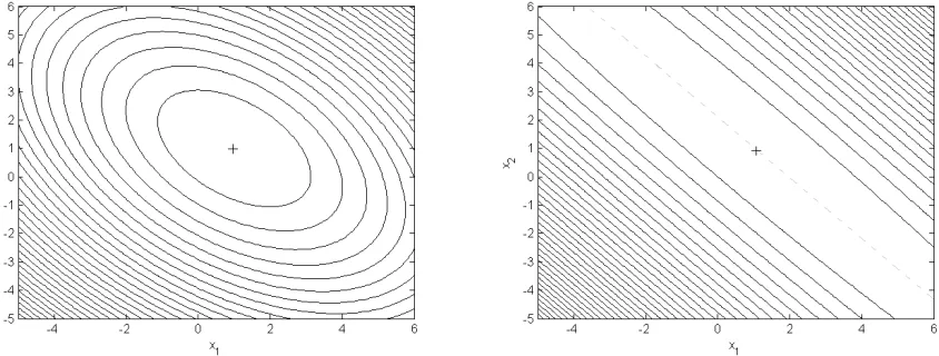
Figure 1.1 compares a well-posed linear least squares problem to an ill-posed problem. The functional plotted on the left is from the well-posed problem and has a nice well-defined minimum. The functional plotted on the right is from the ill-posed problem and does not have such a well-defined minimum. In fact, there is a entire range of values for which the functional is a minimum. Even if (1.3) is an
Figure 1.1: Contours ofkd−F(x)k2
2 for two linear inverse problems. Left: Well-posed problem. Right: Ill-posed problem.
CHAPTER 2
LEAST SQUARES
Least squares is a straightforward, computationally inexpensive method that is widely used to solve inverse problems [15]. Even though regularization is the focus of this thesis, we begin with a discussion of unregularized least squares to establish the framework and notation needed for later chapters. In addition, we will explain and exploit some nice statistical properties of this method in this chapter.
The unregularized least squares estimate ˆx is given as:
J(x) =kd−F(x)k2 2
ˆ
x= arg min x J(x).
(2.1)
In a purely mathematical sense, thearg minabove should bearg inf. However, since all real problems are solved in the computational realm and the numbers accessible to the computer are a finite subset of R, it is valid to use min instead of inf. This convention will be used throughout the rest of the paper.
2.1
Ordinary Least Squares (OLS)
J(x) =kd−Axk22
ˆ
x= arg min x J(x).
(2.2)
This is a quadratic functional and the minimum can be found directly by setting:
∇J =−1
2A T
(d−Ax) = 0. (2.3)
Solving for x gives the ordinary least squares estimate:
ˆ
x= (ATA)−1ATd. (2.4)
If (ATA) is invertible and the problem is well-conditioned, then this is a straightfor-ward way to estimate x. In addition, if we assume that the error ε in the problem from (1.1) is a random variable with a mean of zero, then ˆx is an unbiased estimate of x since the expected value of ˆxis equal to x, i.e.
E(ˆx) =E((ATA)−1ATd) = (ATA)−1ATE(d) = (ATA)−1ATE(Ax+ε) = (ATA)−1ATAx
=x.
(2.5)
2.2
Nonlinear Least Squares
be used. Finding the solution to:
ˆ
x= arg min
x J(x) (2.6)
falls under a whole field of mathematics called optimization. There are many different methods that can be used to solve this nonlinear unconstrained optimization problem including: genetic algorithms, stochastic algorithms, particle swarm optimization algorithms, quantum optimization algorithms (need a quantum computer), pattern search algorithms, direct search methods, steepest descent algorithms, and conjugate gradient algorithm. However, if the function is well-behaved (i.e. continuous and twice differential in the domain), then Newton’s method style algorithms are among the fastest and most efficient, and can even offer quadratic convergence [2, 13].
If we are given a functionf :Rn →
Rnthat is Fr´echet differentiable and a starting
point that is sufficiently close to the root then Newton’s Method estimates the roots of f(x) by iterating
xk+1 =xk+ ∆xk
∆xk=−∇f−1(xk)f(xk)
(2.7)
until some criterion of convergence is reached, assuming that the Jacobian of f(x) is invertible at each xk. Here ∇f−1(xk) represents the inverse of the Jacobian matrix. Applying this to (2.6), if J(x) is locally convex, then a local minimum can be found using Newton’s method to find:
∇J(x) = 0. (2.8)
xk+1 =xk+ ∆xk
∆xk=−∇2J−1(xk)∇J(xk)
(2.9)
where ∇2J(x) is the Hessian of J. However, this classical Newton algorithm is not robust and it has been shown that it can even diverge in some cases [13]. Also, it has several other problems in that the Hessian of J can be difficult to obtain computationally and might not be positive definite at some points. To overcome some of these limitations, there are many modifications of Newton’s method. For example, in the modified Newton method, the step length is scaled at each iteration with a positive scalar ρ. Then the step becomes: ∆x = −ρ∇2J−1∇J and a line search is used at each iteration to find the best ρ [13]. Alternatively, Quasi-Newton methods use an approximation for the Hessian, which is updated at each iteration in a way that ensures that it is positive definite and invertible. Restricted-step methods modify the Hessian by H = ∇2J +λ2I, where λ is chosen to ensure that the H is invertible and to ensure the step ∆xk leads to a reduction in J(x) [13].
2.2.1 Gauss-Newton Method and Levenberg-Marquardt
The Gauss-Newton step is given as:
∆xk=− JkTJk
−1
JkT (d−F(xk)) (2.10)
whereJk is the Jacobian ofF atxk. This is derived from Newton’s method as follows: The first and second Fr´echet derivatives of J are given as:
∇J(x) = 2JkT (d−F(x)) (2.11)
∇2J(x) = 2(JT
kJk+Q(x)) (2.12)
whereQ(x) = m
P
i=1
∇2F
i(x)[d−F(x)]i and∇2Fi(x) is the Hessian of theith component of F(x). Ignoring Q(x) from ∇2J in the Newton iteration gives (2.10). So the Gauss-Newton method approximates ∇2J(x) with just the first-order part JT
kJk. If necessary, the Jacobian can be calculated with finite differences without affecting the performance of the method [2]. The Gauss-Newton method, when it converges, can be more efficient than the full Newton method. It also can ultimately achieve a quadratic rate of convergence [2]. In addition, it usually converges faster and is more efficient than the Quasi-Newton method [2],[13]. However, it is based on the fact that kJkTJkk kQ(x)k, which is true for small residual problems and is not a good approximation when the largest eigenvalue of JTJk is comparable to ||d−F(xk)||22 [2].
Levenberg-Marquardt
(LM) algorithm [13] is a modification of the Gauss-Newton method that allows for singular or ill-conditioned matricesJTJ and takes smaller, safer steps by introducing a parameter λk and a diagonal matrix D with positive diagonal elements:
∆xk =−(JkTJk+λD)−1JkT(d−F(xk)) (2.13)
whereDis a diagonal matrix with positive diagonal elements. For simplicity,D=Iis often used and in this case ∆xk is an interpolation between the steepest descent step and the Gauss-Newton step. Alternatively, a typical choice for D is a matrix with diagonal elements equal to those of JTJ. Note that ∆x = −M−1∇J is guaranteed to be a descent direction as long as M is positive definite [2].
The Levenberg-Marquardt parameter λk is chosen so that J(xk+1) < J(xk). If
λk is too small, then ∆xk might not lead to a reduction in the value of J. If λk is too large, then the algorithm will take small steps and its progress will be slow. A common way to determine λk is as follows: start with a small value for λ1, i.e.
LM algorithm is in general a robust method and works well for many nonlinear least squares problems [2].
2.3
Generalized Least Squares
If the data are of varying scales or if the measurements have different variances, or if the errors in the data are correlated, then these factors can be taken into account in the estimation ofx. Generalized least squares does this by weighting the least squares problem with the inverse of the covariance matrix of the error. The generalized least squares estimate ˆxGLS is:
JGLS(x) =kd−F(x)k2C−1
ε
ˆ
xGLS = arg min
x JGLS(x)
(2.14)
where k d−F(x) k2
Cε−1 is the weighted 2-norm (d−F(x))
TC−1
ε (d−F(x)). This is an intuitive addition to least squares, because if we have some measurements with a large variance then it makes sense that these points should have less weight. Also, if
ε∼N(0, Cε), then ˆxGLS from (2.14) is equivalent to the maximum likelihood estimate.
All the previous least squares results can be applied to the generalized least square estimate by first converting the generalized least squares problem into an OLS problem:
˜
F(x) = Cε−1/2F(x),
˜
d=Cε−1/2d.
(2.15)
ˆ
x= arg min x k
˜
d−F˜(x)k2
2 . (2.16)
We now introduce a theorem describing an important statistical property ofJGLSfrom
(2.14) at its minimum value. This theorem will provide much of the basis needed for the theory developed later in this work.
Theorem 1. IfF :Rm →
Rnis a linear function, andε ∼N(0, Cε), thenJGLS(ˆxGLS)∼
χ2n−m.
Proof. Since F : Rm → Rn is a linear function we can write it as a matrix A with dimension n×m. Also, x∈Rm,d ∈
Rn, and Cε has dimension n×n. So we have:
˜
d=Cε−1/2Ax+Cε−1/2ε
= ˜Ax+ ˜ε.
(2.17)
Theorem 7 in Appendix A implies: ˜ε ∼ N(0,In). Now JGLS(x) = kd˜−Ax˜ k22 and ˆ
xGLS = ˆx= ( ˜ATA˜)−1A˜Td˜, which gives:
kd˜−A˜xˆk22 =kd˜−A˜( ˜ATA˜)−1A˜Td˜k22
=k(In−A˜( ˜ATA˜)−1A˜T) ˜dk22 =k(In−P) ˜dk22.
(2.18)
(In−P) ˜d= (In−P) ˜d−Ax˜ + ˜Ax = (In−P) ˜d−Ax˜ +PAx˜ = (In−P)( ˜d−Ax˜ ) = (In−P)˜ε.
(2.19)
Combining this result and the fact that (In−P) is idempotent and symmetric implies:
kd˜−A˜(ˆx)k22= ˜εT(In−P)˜ε. (2.20)
Theorem 5 from Appendix A says that the rank of a matrix that is idempotent and symmetric is equal to its trace. Using this result:
rank(In−P) =trace(In−P)
=trace(In)−trace(P) =n−trace( ˜A( ˜ATA˜)−1A˜T) =n−trace(( ˜ATA˜)−1A˜TA˜) =n−m
(2.21)
Finally, applying the Theorem 8 from Appendix A:
˜
εT(In−P)˜ε ∼χ2n−m. (2.22)
The use of Theorem 1 to analyze the least squares solution is sometimes called the
CHAPTER 3
REGULARIZATION AND THE
χ
2METHOD
As mentioned in previous chapters, inverse problems are often ill-posed in practice and finding a solution requires some form of regularization. A common way to regularize inverse problems is to add a second term to the functional being minimized in order to stabilize and add uniqueness to the solution. This is known as Tikhonov regularization and this modified functional is sometimes called the Tikhonov functional:
Jtkh(x) =kd−F(x)k2 +α2 kLx−z k2, (3.1)
where L is a linear operatorL:Rm →
Rq,z ∈Rq, and α is a scalar.
The matrix L is commonly chosen to be the identity operator or an approximate first or second derivative operator. If L is the identity, then z could be an initial estimate of x. In this case, the regularization parameter α controls the compromise between how far the solution deviates from the original estimate and how well the solution fits the data. Alternatively, when x is the discretization of a continuous function, then the expected structure ofxcan be exploited by choosingLto represent a derivative operator. In this case,z represents the desired slope in the solution and is often set to be 0 to obtain smooth solutions. In this case, α controls the compromise between how smooth the solution is and how well the solution fits that data.
problem. It is desirable to chooseαso that it changes the original problem just enough that a good estimate forxcan be obtained. Choosing the value ofαthat accomplishes this, however, is not trivial.
3.1
Choice of Regularization Parameter
There is a voluminous amount of literature on how to determine the regularization parameter for linear least squares problems. Common methods include L-Curve, Gen-eralized Cross Validation, and the discrepancy principle. For a complete treatment of these methods, the reader is referred to the literature, specifically [1, 4]. A relatively new method, called theχ2 method, is proposed by Mead in [8] and developed further in [10, 9]. The focus of this thesis is to extend this method for solving nonlinear inverse problems.
3.1.1 Nonlinear Regularization
Regularization methods for linear problems do not straightforwardly extend to non-linear least squares problems. Since the nonnon-linear problems are solved iteratively, the methods for determining the regularization parameter generally breakdown into two approaches.
In the first approach,α remains fixed throughout the nonlinear inversion process. In these methods, the inversion is done multiple times for different values of α until the solution meets some criterion. Some criteria used for evaluating the solution are the discrepancy principle [1] and Generalized Cross Validation (GCV) [3].
procedure has to be integrated with the method for estimating α. Some examples of this type of method include Occam’s inversion and an implementation of GCV as proposed in [3]. The nonlinearχ2 method which uses this second approach and is an alternative to these methods and is developed in this thesis.
3.1.2 Statistical Framework
A popular data assimilation method in weather forecasting based on a Bayesian framework is known as the three-dimensional variational method (3DVAR) [7]. It starts with the following assumptions:
d=F(x) +ε, x=xp+f,
(3.2)
whereε∼N(0, Cε) , f ∼N(0, Cf) andxp is an initial estimate ofx. This differs from traditional inverse problems in that we have both noisy data and a prior probability distribution for the parameter set.
Since both ε, f are normal, it is straightforward to find the maximum a posteriori (MAP) estimate for x for a given data set. The MAP estimate xM is:
xM = arg max
x (P(x|d)), (3.3)
where P(x|d) represents the conditional probability density function for x given the data d. Using Baye’s theorem, it possible to write P(x|d) in terms of prior distributions
P(x|d) = P(d|x)P(x)
where P(x) represents the prior distribution for x, P(d) represents the distribution for d and P(d|x) represents the conditional probability density function for d, given the data x.
So xM becomes:
xM = arg max
x
P(d|x)P(x)
P(d)
. (3.5)
Since ε is normally distributed, P(d|x) can be written as
P(d|x) = 1
2πn2|Cε| 1 2
exp
−1
2(d−F(x)) TC−1
ε (d−F(x))
.
In addition, since the prior distribution is a multivariate normal, that we can write:
P(x) = 1
2πm2|Cf| 1 2
exp
−1
2(x−xp) TC−1
f (x−xp)
.
Using these distributions and the fact that P(d) does not depend on x, the MAP estimate becomes:
xM = arg max
x
exp −1
2(d−F(x)) TC−1
ε (d−F(x))
exp −1
2(x−xp) TC−1
f (x−xp) = arg min
x
(d−F(x))TCε−1(d−F(x)) + (x−xp)TCf−1(x−xp) .
(3.6)
The MAP estimatexM minimizes
JM(x) =||d−F(x)||
2
Cε−1 +||x−xp||
2
Cf−1, (3.7)
which is very similar to the Tikhonov functionalJtkhfrom (3.1) whenLis the identity
respective inverse covariance, whereas in (3.1) the second term is weighted with α2.
3.1.3 Linear χ2 Method
If ε ∼ N(0, σ2
εI) and f ∼ N(0, σ2fI), then xM is identical to the estimate found by
minimizing the Tikhonov functional withL as the identity, z as the initial estimate, and withα=σε/σf. Of course, many times in inverse problems, the prior covariance for f is not available. However, all is not lost. Mead in [8] suggested capitalizing on Theorem 2 to estimate α.
Theorem 2. If F :Rm →
Rn is a linear function and the following holds:
d=F(x) +ε, x=xp+f,
(3.8)
then JM(x) from (3.7) at its minimum value, i.e. JM(xM), follows a χ2 distribution
with n degrees of freedom.
Proof. Since F : Rm →
Rn is a linear function, we can write it as a matrix A with
dimensionn×m. Also,x∈Rm,d∈
Rn,Cεhas dimensionn×nandCf has dimension
m×m.
First, rewrite (3.7) as:
JM(x) =
Cε−1/2(Ax−d)
Cf−1/2(x−xp)
2 2
xM = arg min
x JM(x).
(3.9)
J(x) =
Cε−1/2A
Cf−1/2
x−
Cε−1/2d
Cf−1/2xp
2 2 . (3.10)
For the sake of simplicity, let
A∗ =
Cε−1/2A
Cf−1/2
, d
∗ =
Cε−1/2d
Cf−1/2xp
, ε ∗ =
Cε−1/2ε
Cf−1/2f
. (3.11)
Then:
J(x) =kd∗−A∗xk22
ˆ
x= arg min x J(x),
(3.12)
where A∗ has dimension (n +m)× m, d∗ has dimension (n +m) ×1, and ε∗ ∼ N(0,In+m). By Theorem 1, in the previous chapter, J(ˆx)∼χ2n.
The method proposed in [8] is called the χ2 method and it says choose α such that the minimum of the functional (3.7) has a value that is consistent with its χ2 distribution. This is implemented in [8] as finding the α that makes the minimum of the functional equal to the mean of the χ2 distribution. Also, Mead showed in [8] that Theorem 2 holds asymptotically when ε and f are not normally distributed, which allows this method to be applied in a more general sense.
3.2
χ
2Tests for Gauss-Newton Method
is solved with a sequence of linearizations, then it is possible to find appropriate χ2 tests at each iteration.
The Gauss-Newton method to find xM = arg minxJM(x) from (3.7) is as follows.
First find the first and second Fr´echet derivative of JM,
∇JM(x) =JTC
−1
ε (d−F(x))−C
−1
f (x−xp), (3.13)
where J is the Jacobian of F atx. Now
∇2J
M(x) = JTCε−1J+Q(x) +C
−1
f , (3.14)
where Q(xk) is the second-order information of JM. The Gauss-Newton method
ignores this Q, so we get the following iteration:
xk+1 =xk+ ∆xk ∆xk =− JkTC
−1
ε Jk+Cf−1
−1
JkTCε−1(d−F(xk))−Cf−1(xk−xp)
.
(3.15)
The Gauss-Newton method can be converted to a sequence of linear OLS problems with the following manipulations:
xk+1 =xk+ JkTC
−1
ε Jk+Cf−1
−1
JkTCε−1rk−Cf−1(x−xp)
, (3.16)
where rk=d−F(xk). Now multiplying both sides with JkTCε−1Jk+Cf−1
gives:
JkTCε−1Jk+Cf−1
xk+1 = JkTC
−1
ε Jk+Cf−1
xk+ (JkTC
−1
ε rk−Cf−1(xk−xp)). (3.17)
JkTCε−1Jk+Cf−1
xk+1 = (JkTC
−1
ε Jk)xk+ (JkTC
−1
ε rk+Cf−1xp). (3.18)
Rewrite and factor out JT kC
−1
ε on right-hand side
JkTCε−1Jk+Cf−1
xk+1 =JkTC
−1
ε ((Jkxk+rk) +Cf−1xp). (3.19)
This can be factored again into the normal equations:
Cε−1/2Jk
Cf−1/2 T
Cε−1/2Jk
Cf−1/2
xk+1 =
Cε−1/2Jk
Cf−1/2 T
Cε−1/2(dek)
Cf−1/2xp
, (3.20)
where dek =d−F(xk) +Jkxk. Finally, this can be written as the sequence of linear
OLS problems:
e
Jk(x) = kdek−Jkxk2
Cε−1 +kx−xpk
2 Cf−1 ˆ
xk+1 = arg min x Jek(x)
(3.21)
The sequence of OLS problems in (3.21) solves the following linear inverse problem at each iteration.
e
dk=Jkxk+1+εk,
xk+1 =xp+f
(3.22)
where εk = ε+νk with Cov(εk) = Cεk and νk represents error introduced by the
Theorem 3. If Jek(x) = kdek−Jkxk2
Cε−1 +kx−xpk
2
Cf−1, xˆk+1 = arg minxJek(x), the nonlinear error is zero, and the following are true:
dk=Jkxk+1+εk εk∼N(0, Cεk)
xk+1 =xp+f f ∼N(0, Cf)
(3.23)
then Jek(ˆxk+1)∼χ2n.
Proof. This follows trivially from Theorem 2.
If the nonlinear error is zero, then the problem is likely linear. However, this theorem can still be used to develop theχ2 test for nonlinear problems by making the assumption that Cεk ≈Cε. This approximation will get better as the iterations gets
closer to the solution and the nonlinear error is reduced. Under this assumption, the
χ2 method can be applied at each iterations to achieve increasingly better estimates forCf−1. In the next chapter, we show that this assumption works well for two inverse problems given in [1].
Now we consider a more general case whereL is used as in (3.1). It is not difficult to see that in a similar way we can minimizeJM(x) =kd−F(x)k2C−1
ε +kLx−z k
2 C−f1 with the sequence of linear OLS problems:
e
Jk(x) =kdek−Jkxk2
Cε−1 +kLx−zk
2
Cf−1. (3.24)
Theorem 4. If Jek(x) = kdek−Jkxk2
Cε−1+kLx−zk
2
Cf−1, whereL:R m →
Rq is a linear
operator and xˆk+1 = arg minxJek(x), the invertibility condition holds:
N(Jk)∩ N(L) = 0 where N(A) is the null space of A, the nonlinear error is zero, and the following are true:
dk=Jkx+εk, εk∼N(0, Cεk)
Lx=z+f f ∼N(0, Cf)
(3.25)
Then,Jek(ˆx)∼χ2n−m+q.
Proof. L : Rm → Rq is a linear operator and x ∈
Rm, z ∈ Rq d ∈ Rn, Cε has dimension n×n, and Cf has dimension q×q.
Rewrite as an ordinary least squares problem:
J(x) =
Cε−1/2Jk
Cf−1/2L
x−
Cε−1/2dek Cf−1/2z
2 2 . (3.26)
For sake of simplicity, let
A∗ =
Cε−1/2Jk
Cf−1/2L
, d
∗
=
Cε−1/2dek Cf−1/2z
, ε ∗ =
Cε−1/2ε
Cf−1/2f
. (3.27)
The least squares problem can be written as:
e
Jk(x) =kd∗−A∗xk22, ˆ
x= arg min x J(x),
(3.28)
3.2.1 χ2 Tests for Levenberg-Marquardt Method
Recall that the Levenberg-Marquardt method is a modification of the Gauss-Newton method to help ensure the convergence of the algorithm. The LM step to find xM =
arg minxJM(x) from (3.7) is as follows:
xLMk+1 =xk+ ∆xk, ∆xk =− JkTC
−1
ε Jk+Cf−1+λ 2D−1
JkTCε−1(d−F(xk))−Cf−1(xk−xp)
.
(3.29)
It is possible to write the regularized LM method as a sequence of OLS problems in a similar way as the Gauss-Newton method. These iterates become:
e JLM
k (x) =kdek−Jkx)k2
Cε−1 +kx−xpk
2
Cf−1 +λ
2kD(x−x k)k22,
xLMk+1 = arg min x Je
LM
k (x).
(3.30)
The χ2 test is not clear for this more complicated functional because there is no statistical information about the third term in the functional. However, it is possible to derive an approximate χ2 test for the LM method. First, to simplify the following manipulations, we convert JM(x) into a nonlinear OLS problem. Let:
F(x)∗ =
Cε−1/2F(x)
Cf−1/2Lx
, d
∗
=
Cε−1/2dek
Cf−1/2z , ε ∗ =
Cε−1/2ε
Cf−1/2f
. (3.31)
Then we have the following new problem:
d∗ =F∗(x) +ε∗ where ε∗ ∼N(0,In+q). (3.32)
method, but it is helpful here to derive it in a slightly different way. Consider the Taylor series expansion of F∗ around a point xk:
F∗(x) = F∗(xk) +Jk∗(x−xk) + higher order terms, (3.33)
where Jk∗ is the Jacobian of F∗ at xk. Plugging this back into (3.32), we get:
d∗ =F∗(xk) +Jk∗(x−xk) +ε∗k, (3.34)
whereε∗k=ε∗+νkandνkrepresents the error introduced by ignoring the higher-order terms. Rewriting:
r∗k=Jk∗∆xk+ε∗k, (3.35)
whererk∗ =d∗−F∗(xk) and ∆xk=xk+1−xk. We see that the OLS estimate for ∆xk is
d
∆xk = (Jk∗TJ
∗
k)
−1J∗T k r
∗
k. (3.36)
As in the proof of Theorem 1,
krk∗−Jk∗∆dxkk22 =k(I−P)rkk22,
=k(I−P)ε∗kk2 2,
(3.37)
where P = Jk∗(J∗T k J
∗
k)
−1J∗T
k . Now replace ∆dxk in (3.37) with the LM step ∆xk =
(J∗T k J
∗
k +λ2kDTD)
−1J∗
k(r
∗
k), so
kr∗k−Jk∗∆xkk22 =k(r
∗
k−J
∗
k(J
∗T k J
∗
k+λ 2 kD
TD)−1J∗T k r
∗
kk 2 2
=k(I−Pˆ)rk∗k2 2.
where ˆP = Jk∗(J∗T k J
∗
k + λ2kDTD)
−1J∗T
k . Pˆ is symmetric but it is not idempotent and so is not an orthogonal projection. However, if kJk∗TJk∗k >> kλ2kDTDk, then (Jk∗TJk∗)−1 ≈(Jk∗TJk∗+λ2kDTD)−1 and so ˆP is approximately equal to the projection
P from (3.37). Then,
krk∗−Jk∗∆xkk22 =k(I−Pˆ)r
∗
kk 2 2
≈ k(I−P)rk∗k22
=k(I−P)ε∗kk2 2
∼χ2n (if ε∗k =ε∗).
(3.39)
Now, rewriting:
kr∗k−Jk∗∆xkk22 =kd
∗−
F∗(xk)−Jk∗(x
LM
k+1−xk)k22 =k(d∗−F∗(xk) +xk)−Jk∗x
LM
k+1k 2 2 =
Cε−1/2Jk
Cf−1/2
x
LM
k+1−
Cε−1/2dek Cf−1/2xp
2 2
=Jek(xLMk+1).
(3.40)
So the Gauss-Newton functional Jek at the LM estimate xLMk+1 approximately follows
3.3
Nonlinear
χ
2Method
In Section 3.2 and Theorems 3 and 4, we derived approximate χ2 distributions for the regularized Gauss-Newton functional Jk at ˆxk+1, i.e. Jek(ˆxk+1). Also, in Section
3.2.1, we found an approximate χ2 distribution for
e
Jk(xLMk+1). In keeping with the approach proposed by Mead in [8] for the linear χ2 method, we suggest using these
χ2 distributions to estimate the regularization parameter. However, when solving real problems, only one sample of Jek is available because there is only one realization of
the errorε in the data. Therefore, the best we can do is to use a single characteristic of the distribution to find the regularization parameter.
In [10], they suggest using the mean of theχ2distribution to estimateα. However, for aχ2 distribution the median is approximately equal to the mean. This implies that if a perfectly weightedJek(ˆxk+1) is sampled multiple times, about half of these samples will be greater than the mean. If we estimate the regularization parameter such that
e
Jk(ˆxk+1) is always equal to the mean, then about half of the time the regularization parameter will have to be made smaller to compensate for the realization of data error that makes a perfectly weighted Jek(ˆxk+1) larger than the mean. This means
that choosing α such that Jek(ˆxk+1) is equal to the mean will under regularize the problems about half of the time. To avoid under-regularization, we suggest using the upper bound of the desired confidence interval for the χ2 distribution. For example, if the desired confidence level is 95%, then this upper bound is the number at which a correctly weightedJek(ˆxk+1) will be less than or equal to 95% of the time. We suggest
choosing the regularization parameter such that Jek(ˆxk+1) is equal to this number.
parameter at each Gauss-Newton iteration.
Algorithm 1 Nonlinear χ2 method with Gauss-Newton step Input L, Cε,xp, tol
for k=1,2,3,...do Calculate Jk and dek
Define:
e
Jk(x, α) = kdek−Jkxk2
Cε−1 +α
2kL(x−x p)k22 Choose αk such that:
e
Jk(x, αk)≈Φ−n−1m+q(95%)
where Φ−n−1m+q is the inverse cumulative distribution function (CDF) of χ2 n−m+q.
ˆ
xk+1 = arg min
x Jek(x, αk) = JkTCε−1Jk+α2kL
TL−1
(JkTCε−1dek+α2kLTLxp)
if |JM(ˆxk+1)−JM(xk)|
JM(xk) < tol then
converged andxM = ˆxk+1 return
end if end for
Algorithm 2 Nonlinear χ2 method with LM step Input L, Cε,xp,λ1,D
for k=1,2,3...do Calculate Jk and dek if k >1 then
Define:
e JLM
k (x, λ) =kdek−Jkxk2
Cε−1 +α
2
kkL(x−xp)k22+λ
2kD(x−x k)k22
xLM
k+1 = arg min x Je
LM
k (x, λ) = JkTCε−1Jk+α2kL
TL+λ2 kD
−1
(JkTCε−1dek+α2kLTLxp+λ2kxk)
Update LM parameter by finding a smallλk+1 that still ensures
JM(xLMk+1)<JM(xLMk ) end if
Define:
e JLM
k (x, α) = kdek−Jkxk2
Cε−1 +α
2kL(x−x
p)k22+λ2kkD(x−xk)k22
e
Jk(x, α) = kdek−Jkxk2
Cε−1 +α
2kL(x−x p)k22 Choose αk+1 such that:
e
Jk(xLMk+1, αk+1)≈Φ−n−1m+q(95%)
where Φ−n−1m+q() is the inverse CDF of χ2n−m+q.
xLM
k+1 = arg minxJekLM(x, αk+1): if |JM(xLMk+1)−JM(xLMk)|
JM(xLMk+1) < tol then
converged andxM =xLMk+1 return
Algorithm 2 has the additional complication of determining the LM parameter
λk. This can be found using the methods from the LM implementations discussed in Chapter 2. This algorithm has more computational overhead than the previous algorithm, but this is simply the price for a more robust method that is needed to solve more difficult problems.
3.3.1 Numerical Implementation of Algorithms
In Algorithm 1 and 2, it is necessary to do some type of line search at each iteration to find αk+1. To do this, any standard root finding algorithm can be used such as the bisection method, inverse quadratic interpolation, secant method, or Newton’s method. In [10], the authors introduce an exact Newton root-finding algorithm that uses SVD of the linear inverse problem which would work for Algorithm 1.
In Algorithm 1 and 2, the Gauss-Newton method and the Levenberg-Marquardt method are written as a sequence of OLS problems. Since the algorithms require that these OLS problems to be solved multiple times at each iteration, it is important that the OLS solution is computed in an efficient matter. We saw in Chapter 2 that the OLS estimate is given as:
ˆ
x= arg min
x kd−Axk 2 2,
ˆ
x= (ATA)−1ATd.
(3.41)
implementation of QR factorization to solve overdetermined problems [11].
Also, in many of the previous equations the inverse of the square root of the covariance matrix is taken in order to factor the steps into an OLS problem. When the matrix is a diagonal matrix this operation is trivial. However, if the covariance matrices have nonzero off-diagonal elements, taking the matrix square root can be expensive and unstable. Instead of taking the matrix square root, we can split the matrix with Cholesky factorization, which can be more accurate and computationally cheaper. The following example shows why this is valid. If we have
d=Ax+ε ε∼N(0, Cε) (3.42)
and if R represents the Cholesky decomposition of Cε, i.e. RRT = Cε, then we can normalize the problem using R:
R−1d =R−1Ax+R−1ε. (3.43)
If we let ˜A = R−1A, ˜d = R−1d, and ˜ε = R−1ε, then Theorem 7 in Appendix A implies: ˜ε ∼N(0,In) and (3.43) becomes the normalized OLS problem:
˜
CHAPTER 4
APPLICATION, SOLUTIONS, AND NUMERICAL
EXPERIMENTS
In this chapter, we consider two ill-posed nonlinear inverse problems and use these problems to test the theorems and algorithms developed in Chapter 3. These test problems are from Chapter 10 of [1] where the authors both describe problems and provide the corresponding solutions. Conveniently, the authors included Matlab codes along with the text that set up the forward problem and solve the inverse problems with existing methods. This allowed us to recreate their results and use them as a basis for comparison.
4.1
Nonlinear Cross-Well Tomography
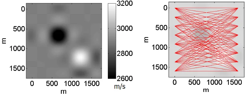
The first problem is an implementation of nonlinear cross-well tomography. The forward model includes ray path refraction where the refracted rays tend to travel through high-velocity regions and avoid low-velocity regions, which adds nonlinearity to the problem. The problem is set up with two wells spaced 1600 m apart, and there are pairs of sources and receivers at equally spaced depths down the wells. The travel time between each pair of opposing sources and receivers is recorded, and the objective is to recover the two-dimensional velocity structure between the two wells. The true velocity structure has a background of 2.9 km/s with an embedded Gaussian shaped region that is about 10% faster than the background and another Gaussian-shaped region that is about 15% slower. The observations for this particular problem consist
Figure 4.1: The setup of the cross-well tomography problem. (Left) Shown here is the true velocity model(m/s). (Right) The ray paths crossing through region of interest (background is faded to make the ray paths more clear).
64 model parameters (the slowness of each block) and 64 observations (the ray path travel times).
4.1.1 Numerical Experiments
In Chapter 3, it was shown that the Gauss-Newton method can be written as the sequence of linear inverse problems:
e
Jk(x) = kdek−Jkxk2
Cε−1 +kx−xpk
2 Cf−1
xk+1 = arg min x Jek(x)
(4.1)
and the assertion was made that Jek(xk+1) approximately follows a χ2n distribution.
To test this assertion, we carried out the following numerical experiment. First, we generated a set of synthetic data from an initial parameter set. Then we added 1000 different realizations of ε and f to the synthetic data and initial parame-ters, respectively. The added noise ε was sampled from N(0,(.001)2I
64) and f from N(0,(.00001)2I
64). For perspective, the values fordare O(.1) and the values for xare
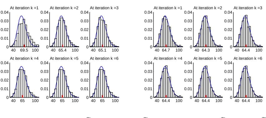
O(.0001). This means the data had about 1% noise added and the initial parameter estimate had 10% noise added. We then used the Gauss-Newton method to solve the nonlinear inverse problem 1000 times, once for each realization of noise. Essentially, this is equivalent to sampling Jek(xk+1) 1000 times. Each of these converged in 6
iterations. A histogram of these samples of Jek(xk+1) at each iteration is given below in Figure 4.2. Since there are 64 observations and 64 model parameters, the theory says that Jek ∼χ264 and so E(Jek(xk+1)) = 64.
In [1] the authors use a discrete approximation of the Laplacian operator 4e to
becomes:
e
Jk(x) = kdek−Jkxk2
C−ε1 +kLx−0k
2 Cf−1,
xk+1 = arg min
x Jek(x).
(4.2)
Using this operator and the same assumptions as above, we found approximate distributions of Jek when L = 4e. The approximate distributions found are shown
in Figure 4.2. In the top-left histogram in Figure 4.2 the sampled distribution of
e
Jk(xk+1) for the first iteration is shifted slightly right of the theoreticalχ2distribution predicted in Theorem 3. This is what would be expected if Cε underestimates Cεk.
40 69.5 100 0 0.01 0.02 0.03 0.04
At iteration k =1
40 65.4 100 0
0.01 0.02 0.03 0.04
At iteration k =2
40 65.1 100 0
0.01 0.02 0.03 0.04
At iteration k =3
40 65 100 0
0.01 0.02 0.03 0.04
At iteration k =4
40 65 100 0
0.01 0.02 0.03 0.04
At iteration k =5
40 65 100 0
0.01 0.02 0.03 0.04
At iteration k =6
40 64.7 100 0
0.01 0.02 0.03 0.04
At iteration k =1
40 64.3 100 0
0.01 0.02 0.03 0.04
At iteration k =2
40 64.4 100 0
0.01 0.02 0.03 0.04
At iteration k =3
40 64.4 100 0
0.01 0.02 0.03 0.04
At iteration k =4
40 64.4 100 0
0.01 0.02 0.03 0.04
At iteration k =5
40 64.4 100 0
0.01 0.02 0.03 0.04
At iteration k =6
Figure 4.2: Histograms ofJek(xk+1). (Left): Jek with L= I, (Right): Jek with L=4e.
The mean of the sample is shown as the middle tick, and χ264 probability density function is shown as the solid blue line.
4.1.2 Inversion Results
In [1] the authors solve the nonlinear tomography problem by minimizing
JM(x) =kd−F(x)k2C−1
ε +α
2 kLx−0k2, where L=
e
4and the discrepancy principle is used to estimate α. They implemented the discrepancy principle as finding α so thatJdata(xM) =kd−F(xM)k2C−1
ε =m. The data used in this inversion was created by
generating synthetic data from the “true” parameter set and adding a realization of random noiseε to this synthetic data. We use this same approach and data to solve the inverse problem by minimizingJM(x) =kd−F(x)k2C−1
ε +α
2 kL(x−x
p)k2, where
L= I. We did this to create another case to which to compare theχ2 method. Using the same data set, we found solutions using Algorithm 1 from Chapter 3 with both
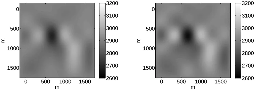
L=4e and forL= I. The solutions found with L=4e and the discrepancy principle
are plotted in Figure 4.3 next to the solution found with L = 4e and Algorithm
the solution found with the discrepancy principle. The solutions found with both methods using L = I are plotted next to each other in Figure 4.4. These are also very similar to each other. It is evident from these figures that solutions found with
L=4e are smoother than the solutions found with L= I.
m
m
0 500 1000 1500
0 500 1000 1500 2600 2700 2800 2900 3000 3100 3200 m m
0 500 1000 1500
0 500 1000 1500 2600 2700 2800 2900 3000 3100 3200
Figure 4.3: Solutions found for the tomography problem with L=4e (Left) Solution
found using the discrepancy principle. (Right) Solution found with Algorithm 1.
m
m
0 500 1000 1500
0 500 1000 1500 2600 2700 2800 2900 3000 3100 3200 m m
0 500 1000 1500
0 500 1000 1500 2600 2700 2800 2900 3000 3100 3200
Figures 4.3 and 4.4 are the results from only one realization of ε. In order to establish a good comparison, the above procedure for both the discrepancy principle and for Algorithm 1 was repeated for 200 different realizations of ε. The mean and standard deviation of ||xM − xtrue||/||xtrue|| for the 200 trials for each method are given below in Table 4.1. Using this as the basis for comparison, χ2 method gave better results on average when L = I. But the discrepancy principle did better on average when the regularizing operator L = 4e. While these differences are
only incremental, the χ2 method was faster computationally because it only solves the inverse problem once and dynamically estimates αk. The discrepancy principle requires the inverse problem to be solved multiple times, incurring computational cost. In this test problem, we replaced the brute line search in the code for the discrepancy principle with a secant iteration, which typically converged in 6 or 7 iterations. The inner iteration typically converged in same number of iterations as Algorithm 1. So the discrepancy principle required 6 or 7 times more forward function evaluations than Algorithm 1. However, Algorithm 1 does a search at each iteration to estimateαk, which doesn’t require more forward function evaluations but does add some computational cost. The net result was that Algorithm 1 was about three times faster in terms of wall-clock time.
Table 4.1: Comparison of discrepancy principle toχ2 method on the cross-well tomog-raphy problem,µ=mean(||xM−xtrue||/||xtrue||),σ =sqrt(var(||xM−xtrue||/||xtrue||))
Method L= I L=4e
χ2 Method µ= 0.01628 µ= 0.0206
σ = 0.0006 σ= 0.00456 Discrepancy Principle µ= 0.01672 µ= 0.018
4.2
Subsurface Electrical Conductivity Estimation
The second problem considered is the estimation of soil electrical conductivity profile from above-ground electromagnetic induction measurements. The forward problem models a Geonics EM38 ground conductivity meter that has two coils on a 1 meter long bar. Alternating current is sent in one of the coils which induces currents in soil and both coils measure the magnetic field that is created by the subsurface currents. For a complete treatment of the instrument and corresponding mathematical model see [5]. Measurements are taken at 9 different heights above the soil and with two different orientations of the instrument, resulting in a total of 18 observations. The subsurface electrical conductivity of the ground is discretized into 10 layers, 20 cm thick, with a semi-infinite layer below 2m, resulting in 11 conductivities to be estimated. An illustration of the setup of this problem is given in Figure 4.5.
4.2.1 Numerical Experiments
We found in solving this inverse problem, the Gauss-Newton method does not always converge. Therefore, finding the solution necessitated the use of the Levenberg-Marquardt algorithm. This provided the opportunity to test the validity of the ap-proximations discussed in Section 3.2.1. In that section, it was shown thatJek(xLMk+1) = kdek−JkxLMk+1k22+kxLMk+1−xpk22 approximately followsχ2n distribution. Once again we
ran some numerical experiments to test this. In a similar way as before, we generated a synthetic data set from a set of parameters and then added 1000 realizations of noise to this data and parameters. This added noiseεwas sampled from N(0,(1)2I
18) andf from N(0,(100)2I
11). For perspective, the values fordare O(100) and the values forx areO(100). This means the data had about 1% noise added and the initial parameter estimate had 100% noise added. We then used the Levenberg-Mardquardt method to solve the regularized nonlinear inverse problem 1000 times for each realization of noise and recorded the samples of Jek(xLMk+1). All of these LM iterations converged
within 6 iterations. Histograms of these 1000 samples of Jk(xLMk+1) are shown below in Figure 4.6. There were 18 observations for this problem and 11 parameters so
E(Jek(xLMk+1)) = 18.
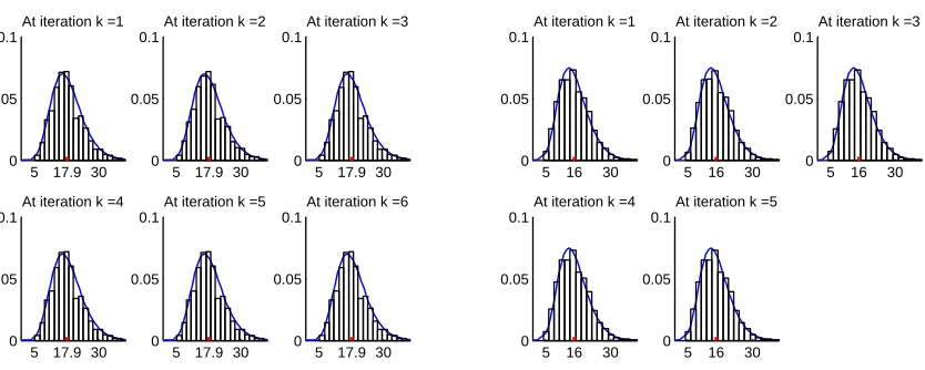
In [1] the authors solve this inverse problem using an approximate 2nd order differential operator L = De(2) to regularize the inversion. We carried out the same
experiment as above, except using this operator to regularize the problem. This matrix L has dimension 9 × 11 so E(Jek(xLMk+1)) = 16. Also, in this experiment, f was sampled from N(0,(10)2I
5 17.9 30 0
0.05 0.1
At iteration k =1
5 17.9 30 0
0.05 0.1
At iteration k =2
5 17.9 30 0
0.05 0.1
At iteration k =3
5 17.9 30 0
0.05 0.1
At iteration k =4
5 17.9 30 0
0.05 0.1
At iteration k =5
5 17.9 30 0
0.05 0.1
At iteration k =6
5 16 30 0
0.05 0.1
At iteration k =1
5 16 30 0
0.05 0.1
At iteration k =2
5 16 30 0
0.05 0.1
At iteration k =3
5 16 30 0
0.05 0.1
At iteration k =4
5 16 30 0
0.05 0.1
At iteration k =5
Figure 4.6: Histograms of Jek(xk+1). (Left) Jek withL= I, (Right) Jek with L=De(2).
The mean of the sample is shown as the middle tick, and theχ2
18,χ216density functions are shown as the solid blue line.
coincided closely with the theoretical χ2 distributions also plotted. This suggests that the approximations used in Section 3.2.1 are good approximations, at least for this problem.
4.2.2 Inversion Results
The inverse problem was also solved in [1] using Occam’s Inversion method. Occam’s Inversion is given as the following algorithm.
Algorithm 3Occam’s Inversion Start with an initial estimate xp for k=1,2,3,...do
DefinexOC
k+1 = JkTC
−1
ε Jk+α2kLTL
−1
(JT kC
−1 ε dek)
Choose largest value of αk such the kd−F(xOCk+1)kCε−1 ≤m
If no such αk exists, then chose a αk that minimizes kd−F(xOCk+1)kCε−1
Stop when kd−F(xOC
k+1)kCε−1 =m
end for
In this implementation of Occam’s Inversion, L was chosen to beDe(2). As in the
previous problem, the data used in this inversion was created by generating synthetic data from the “true” parameter set and adding a realization of random noise ε to this synthetic data. The solution found using this algorithm and data set is plotted in Figure 4.7. We implemented Occam’s inversion using L= I to solve this problem, however, the algorithm diverged with this choice for L.
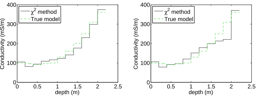
We used the same data set and Algorithm 2 to find the solution using both L= I and L = De(2). These solutions are plotted below in Figure 4.8. Comparing the
solutions found using L = De(2) for the both the χ2 method and Occam’s inversion
in Figures 4.7 and 4.8, it is apparent that both estimate the true solution fairly well for this realization of ε. While the χ2 method was still able to find a solution with
0 0.5 1 1.5 2 2.5 −4000 −2000 0 2000 4000 6000 depth (m) Conductivity (mS/m) LM solution True model
0 0.5 1 1.5 2 2.5
0 100 200 300 400 depth (m) Conductivity (mS/m) Occam’s inversion True model
Figure 4.7: (Left) The unregularized solution. (Right) The solution found with Occam’s inversion.
0 0.5 1 1.5 2 2.5
0 100 200 300 400 depth (m) Conductivity (mS/m)
χ2 method
True model
0 0.5 1 1.5 2 2.5
0 100 200 300 400 depth (m) Conductivity (mS/m)
χ2 method
True model
Figure 4.8: The parameters found using the χ2 method. (Left) L = De(2) (Right) L=I.
Once again, in order to establish a good comparison, each of these methods were run for 200 different realizations of ε. The mean and standard deviation of ||xM −
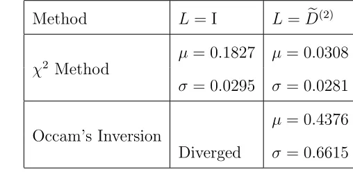
Occam’s inversion was able to find good solutions for some realization of ε, such as the solution plotted in Figure 4.7, the results in Table 4.1 indicate that sometimes it found poor estimates. The mean of||xM−xtrue||/||xtrue||for theχ2 method is almost an order or magnitude smaller than for Occam’s inversion for this problem. Even the χ2 method with L = I found better solutions on average. Also, the relatively small values for σ in Table 4.2 for the χ2 method suggest that the solutions found were fairly consistent with each other. Conversely, the large value of σ in Table 4.1 for Occam’s inversion indicates that these solutions were not consistent with each other. Since both methods estimate the regularization parameter dynamically, the computational cost should be about the same and both methods took about the same speed in terms of wall-clock time.
Table 4.2: Comparison of the χ2 method to Occam’s inversion for the estimation of subsurface conductivities, µ = mean(||xM −xtrue||/||xtrue||), σ = sqrt(var(||xM −
xtrue||/||xtrue||))
Method L= I L=De(2)
χ2 Method µ= 0.1827 µ= 0.0308
σ = 0.0295 σ= 0.0281
Occam’s Inversion
CHAPTER 5
CONCLUSIONS AND FUTURE WORK
We presented a method regularizing nonlinear inverse problems that we call the nonlinearχ2 method. This approach uses statistical information about the data to de-termine the proper level of regularization and is an extension of the linearχ2 method proposed by Mead in [8]. The χ2 tests used in the linear χ2 method were extended to nonlinear problems in Section 3.2. The χ2 method was extended to nonlinear problems using the Gauss-Newton method and the Levenberg-Marquardt method in Algorithms 1 and 2, respectively. We gave numerical results in Sections 4.1.1 and 4.2.1 illustrating the statistical theory developed in Chapter 3 and demonstrated that it was valid for two complex nonlinear problems
Two new algorithms were implemented on two nonlinear problems from [1] and compared against several existing methods for nonlinear regularization. It was shown that Algorithm 1 provided parameter estimates that were of similar accuracy as the discrepancy principle in a nonlinear cross-well tomography problem from [1]. In a subsurface electrical conductivity problem from [1], Algorithm 2 proved to be more robust than Occam’s inversion, providing parameter estimates without the use of a smoothing operator. Algorithm 2 also provided much better estimates than Occam’s inversion on average when the smoothing operator was used.
and this is where the χ2 method prevails. The discrepancy principle solves the nonlinear inverse problem several times for different regularization parameters and thus it requires more forward model evaluations, making it computationally expensive. The nonlinear χ2 method is cheaper because it only solves the inverse problem once and dynamically updates the regularization parameter.
REFERENCES
[1] Richard C. Aster, Brian Borchers, and Clifford H. Thurber. Parameter Estima-tion and Inverse Problems. Elsevier Academic Press, 2005.
[2] Philip E. Gill, Walter Murray, and Margaret H. Wright. Practial Optimization. Academic Press, 1981.
[3] Eldad Haber and Douglas Oldenburg. A GCV based method for nonlinear ill-posed problems. Computational Geosciences, 4(1):41–63, 2000.
[4] Per Christian Hansen.Discrete Inverse Problems, Insight and Algorithms. SIAM, 2010.
[5] B; Corwin D L; Lesch S M; et al Hendrickx, J M H; Borchers. Inversion of soil conductivity profiles from electromagnetic induction measurements: Theory and experimental verification. Soil Science Society of America Journal, 66(3):673– 685, 2002.
[6] Enting Ian G. Inverse Problems in Atmospheric Constituent Transport. Cam-bridge University Press, 2002.
[7] John M. Lewis, S. Lakshmivarahan, and Sudarshan Dhall. Dynamic Data Assimilation. Cambridge University Press, 2006.
[9] Jodi L Mead;. Discontinuous parameter estimates with least squares estimators. Applied Mathematics and Computation, In Revision, 2011.
[10] Jodi L Mead and Rosemary A Renaut. A Newton root-finding algorithm for estimating the regularization parameter for solving ill-conditioned least squares problems. Inverse Methods, 2009.
[11] Cleve Moler. Numerical Computing with Matlab. SIAM, 2006.
[12] Sybil P Parker. McGraw-Hill dictionary of scientific and technical terms. New York : McGraw-Hill, 1994.
[13] G. A. F. Seber and C. J. Wild. Nonlinear Regression. Wiley, 2003.
[14] George A.F. Seber and Alan J. Lee. Linear Regression Analysis. John Wiley and Sons, Inc, 2003.
APPENDIX A
ADDITIONAL THEOREMS
For the convenience of the reader, we include some distribution theory and linear algebra that was used in the proofs of the Theorems 1, 2, 3, and 4 in Chapters 2 and 3. Theorems 5, 6, and 7 are from [14]. The last theorem listed here, Theorem 8, is an important theorem that gives χ2 distribution of a variable that arises in the proof of Theorem 1 in Chapter 2. Since understanding Theorem 8 is helpful in establishing an intuitive understanding of much of theχ2 theory presented in this thesis, its proof is included here.
Theorem 5. If P is symmetric and idempotent matrix then rank(P) = trace(P). (Theorem A.6.2 [14])
Theorem 6. Let A be a symmetric matrix. Then A has r eigenvalues equal to 1 and the rest equal to zero iff A2 =A and rank A=r. (Theorem 2.7 [14])
Theorem 7. Let Y be normal random vector with dimension n×1 with mean µand variance Σ, i.e. Y ∼N(µ,Σ), and let C be an m×n matrix of rank m and d be an
Theorem 8. Let Y be normal random vector with dimension n×1with mean 0 and varianceIn, i.e. Y ∼N(0,In) and letAbe a n×n symmetric idempotent matrix with rank r, then YTAY ∼χ2r.
Proof. Since A is symmetric, it can be written in terms of its spectral decomposition:
A=TTDT where is D is a diagonal matrix whose entries are the eigenvalues of A and T is an orthogonal matrix. Then YTAY =ZTDZ, whereZ =TTY. By Theorem 7,
Z ∼N(0,In). Since A is symmetric, idempotent, and with rank r, Theorem 6 implies that A has r unit eigenvalues and the rest are zero. So YTAY = ZTDZ = Pr
i=1
T2 i. Thus YTAY is equal to the sum of r squared standard normal random variables, so