A Nonlinear Ship Wave Solution Method

(1)

University of New Orleans University of New Orleans

ScholarWorks@UNO

University of New Orleans Theses and

Dissertations Dissertations and Theses

Fall 12-20-2013

A Nonlinear Ship Wave Solution Method

Li Chen

[email protected]

Follow this and additional works at: https://scholarworks.uno.edu/td

Recommended Citation Recommended Citation

Chen, Li, "A Nonlinear Ship Wave Solution Method" (2013). University of New Orleans Theses and Dissertations. 1727.

https://scholarworks.uno.edu/td/1727

This Thesis is protected by copyright and/or related rights. It has been brought to you by ScholarWorks@UNO with permission from the rights-holder(s). You are free to use this Thesis in any way that is permitted by the copyright and related rights legislation that applies to your use. For other uses you need to obtain permission from the rights-holder(s) directly, unless additional rights are indicated by a Creative Commons license in the record and/or on the work itself.

(2)

A Nonlinear Ship Wave Solution Method

A Thesis

Submitted to the Graduate Faculty of the University of New Orleans In partial fulfillment of the Requirements for the degree of

Master of Science

In Naval Architecture and Marine Engineering

By Li Chen

(3)

List of Figures

Fig 2.1: Potential force field ... 6

Fig 2.2: Different connected region ... 7

Fig 2.3: Nomenclature used to define the potential flow problem ... 10

Fig 4.1: Call tree of the program ... 29

Fig 4.2: The initial panel layout ... 29

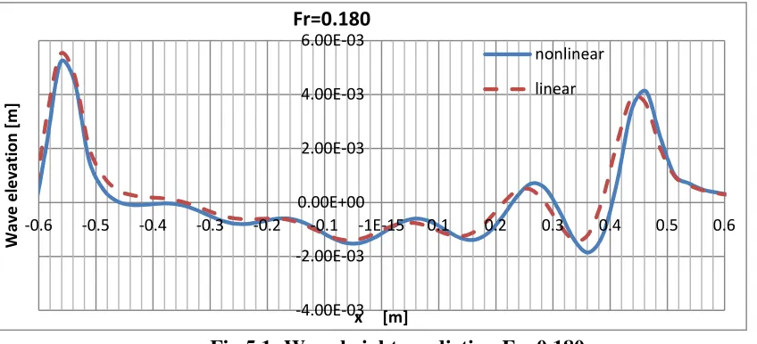
Fig 5.1: Wave height prediction Fr=0.180 ... 33

Fig 5.2: Wave height prediction Fr=0.350 ... 34

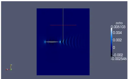
Fig 5.3: Linear method wave pattern Fr=0.180 ... 34

Fig 5.4: Nonlinear method wave pattern Fr=0.18 ... 35

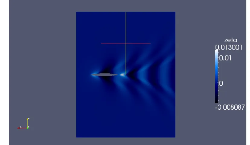
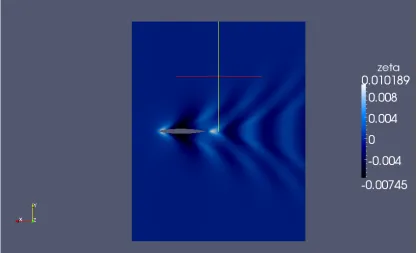
Fig 5.5: Linear method wave pattern Fr=0.350 ... 35

Fig 5.6: Nonlinear method wave pattern Fr=0.350 ... 36

Fig 5.7: Transome wave profile Fr=0.350 ... 36

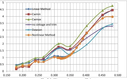
Fig 5.8: Wave resistance coefficient ... 37

(5)

Abstract

Wave resistance on the hull is a major part of the total resistance. In ship design, we want to predict ship wave resistance and the wave pattern for a proper hull form at different velocities. This thesis is an attempt to build up the numerical model for a nonlinear Boundary Element Method similar to RAPID method of Hoyte C. Raven using Wigley hull as the test model of the program.

The RAPID method is known to have a higher accuracy than linearised codes because it closely models the full nonlinear free surface. These computations are carried out via an iterative procedure with convergence criteria using the residual error in the boundary conditions. This method is known to be superior to the convergence criteria of other nonlinear methods which only check that changes in the free surface become small. Comparisons between the linear and nonlinear codes show the nonlinear method to give better wave resistance results.

(6)

Chapter 1 Introduction

During Fall semester 2012, I participated in a graduate level course NAME 6160 Numerical Methods in Hydrodynamic offered by Dr. Lothar Birk, in Naval Architecture and Marine Engineering. That is the first time I get inside the world of Computational Fluid Dynamic(CFD). In our problem, we are using Boundary Element Method (BEM) in solving linearised free surface potential flow problem. The advantage of using BEM is change a three dimensional problem into a two dimensional problem. This method will save a lot of memory we are using in computer in solving the problem. And it is pretty amazing when we see the result of the ship wave propagation.

In practical, the resistance of a ship in still water is mainly consider aspect in ship design. Wave resistance takes over from 10 to 60 % of the total resistance of a ship in still water in the practical cases. While at relatively low speeds the wave resistance is actually zero, as the speed growing up it increases very quickly. A good CFD program can reduce 2% to 3% of the total resistance, that means we can save a lot of the energy during the life time of a ship. As we want to calculate for a more accurate result, I decided to further my study in Hoyte C. Raven's RAPID method, which is nonlinear Boundary Element Method and also a commercial CFD program in Maritime Research Institute Netherlands (MARIN).

We are using Fortran as the programming language in solving the problem. As Fortran is very stable and still very powerful in solving numerical problems. The concept of nonlinear method is based on linear method, except we are updating the parameter we are calculating in each iteration. In the following, we will discuss the theory and the concept in detail. Chapter 2 is the theoretical background of the problem. We eliminate some insignificant phenomena. Then use the mathematical theory we derived on class to transform our problem into a specific numerical problem. Detail derive of the free surface boundary condition will be available in this chapter

In Chapter 3 we describe how to build up the numerical model using the mathematical background we describe in the Chapter2.

(7)

(8)

Chapter 2 Theoretical Background

2.1 Limitation of the problem

We set the coordinate system fixed to the ship hull in still water. The ship is supposed to move straight forward with constant speed. Compare to the real situation, we have neglect some of the aspects. From Raven (1996).

Because different phenomena are governed by multiple physical laws and their theoretical prediction requires quite different mathematical models. For precise prediction methods, we split different phenomena into different mathematical problems. In our discussion here, we will neglect some of the phenomena and it presents as followed:

First of all, the propulsion effects will be disregarded. As the modeling of the propulsion effects are quite different from that we dealt with here, and the situation we are modeling here is consider the ship being towed. The neglect of propulsion may affect the prediction of stern waves, trim and sinkage.

Furthermore, we neglect the wave breaking effects. The physical description of wave breaking in present is still not completed, and no direct or indirect treatment of wave breaking is available for the problem considered. Fortunately only some of the case will have wave breaking in practical, though almost always present, it has relatively minor effect on the problem.

For similar reasons the spray effects will be neglected. Again, for most cases the neglect of spray will also have minor effect on the problem we discuss here.

The trim and sinkage are let out of account. As we are not going to consider the dynamic effect on the ship hull.

Viscous effects will provide little problem for slender hull which we discuss here, but we will have to consider viscous effects for transom stern ship hull.

(9)

After we limit the problem into a certain area, we will use the basic equation as followed.

2.2 Basic Equation

As the continuity equation (conservation of mass) and Navier - Stokes Equations (momentum equations) are the basic fluid mechanic equation we are using here. We will briefly describe these equations.

Starting with the continuity equations we have

dV + Td 0

V S

v S

t ρ ρ

∂

=

∂

∫∫∫

∫∫

(2-1)

d 0

V

D

V

Dt

∫∫∫

ρ = (2-2)

( ) 0

T

v t

ρ _ρ

∂

+ ∇ =

∂

(2-3)

0

T

D

v Dt

ρ _ρ

+ ∇ = (2-4)

In the equations, v is the flow velocity vector. And equations above are the continuity equation in different forms. For equation (2-1) is the integral, conservation form, for finite control volume V fixed in space. Equation (2-2) is the integral, non-conservation form, for finite control volume moving with the fluid. Equation (2-3) is the differential, conservation form, for infinitesimal fluid element fixed in space. Equation (2-4) is the differential, non-conservation form, for infinitesimal fluid element moving with the fluid. The detail derive of the equation will be available in Birk(2012).

Assuming the fluid is incompressible, with constant density ρ=const, we get the continuity

equation (2-3) for incompressible flow

0 T

v

∇ = (2-5)

For the Navier-Stokes equation, let us consider the flow temperature in the fluid to be constant. And the dynamic viscosity of water µ is largely depended on the temperature, therefore we can considerµ to be a constant. Then the Navier-Stokes equation becomes

1

( ) f P ( )

3

T T

v

v v v v

t

ρ_∂ + ∇ _=ρ − ∇ + ∆ +µ µ∇ ∇ ∂

  (2-6)

Now we substitute the continuity equation (2-5) into equation (2-6) yields

1

( T ) f P

v

v v v

t ρ ν

∂

+ ∇ = − ∇ + ∆

∂ (2-7)

in the equation ν is the kinematic viscosity and kinematic viscosity

. The last term of

(10)

If we assume the fluid to be inviscid, as we are considering slender ship hull, with viscosityµ

= 0. Then equation (2-7) becomes

1

( T ) f P

v

v v

t ρ

∂ ₊ _∇ _{= − ∇}

∂ (2-8)

Equation (2-8) is known as Euler equations. We can obtain another useful form of the Euler

equations by rearranging the convective acceleration term ( )

T

v ∇ v_{, from Birk(2012).}

2

1

( ) ( )

2

T

v ∇ v = ∇_ v _− × ∇×v v

  (2-9)

Substituting the rearranged convective acceleration term (2-9) into the Euler equations (2-8) we get

2

1 1

( ) f P

2 v

v v v

t ρ

∂ _{+ ∇} _{− × ∇×} _{= − ∇}

 

∂   (2-10)

We will assume the flow in the fluid to be irrotational, then for irrotational flow the curl of

the velocity becomes∇×v=0. Then the Euler equation becomes

2

1 1

f P

2 v

v

t ρ

∂ _{+ ∇} _{= − ∇}

 

∂   (2-11)

After we compute the velocity field in the fluid, we will use equation (2-11) to compute for the pressure distribution.

2.3 The Laplace Equation

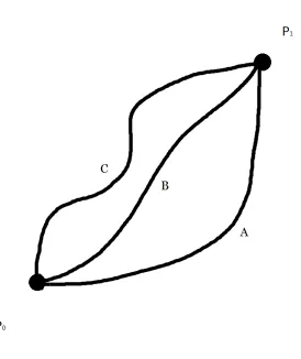
In physics it was discovered that certain force fields have a special property. The work done to move a body from point P0 to point P1 is independent from the path taken, see Fig 2.1. These force field are called conservative and the work done may be computed by computing the difference in potential between point P0 and point P1. The potential is a scalar function representing the conservative vector field. A simple example: [E = -gz] is the potential of the gravity field. In the equation, g is the gravitational acceleration and z is the distance measured from the earth center. The work W per unit mass needed to move a body from P0 = (x0, y0, z0) to P1 = (x1, y1, z1) is W = E1 - E2 = -g(z1 - z0), from Birk (2012).

(11)

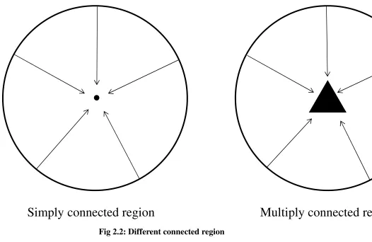
To be precise rot f =0 has to be enforced only in simply connected regions. A simply connected region is a region where all closed curves are reducible. For example, the region can be contracted to a point without leaving the region, see Fig 2.2.

We apply the concept of a pote

with rot v =0 in simply connected regions a velocity potential the equation Φ is a scalar function and its gradient represent th

Fig 2.1: Potential force field

has to be enforced only in simply connected regions. A simply connected region is a region where all closed curves are reducible. For example, the region can be contracted to a point without leaving the region, see Fig 2.2.

We apply the concept of a potential to the velocity field of an irrotational flow. For a flow in simply connected regions a velocity potential Φ exists with

is a scalar function and its gradient represent the velocity field.

has to be enforced only in simply connected regions. A simply connected region is a region where all closed curves are reducible. For example, the region

(12)

Fig 2.2: Different connected region

If we assume the flow is irrotational flowrot v =0, as we select the region around the object but not include the object, we have

v = ∇ Φ _(2-12)

Now we can recall the continuity equation (2-5) for incompressible flow we described earlier

) 0

(

T

v

∇ = (2-13)

We substitute continuity equation(2-13) into potential equation (2-12), then the equation becomes

) 0 ( T

∇ ∇Φ = (2-14)

2

0

∇ Φ = (2-15)

0

∆Φ = (2-16)

Now we have the Laplace equation (2-16) and the Laplace equation is Cartesian coordinates becomes

2 2 2 2 2 2 0

x y z

∂ Φ ∂ Φ ∂ Φ ∆Φ =

∂ + ∂ + ∂ = (2-17)

The Laplace equation is linear and partial differential equation of second order, and it is a special case for continuity equation in inviscid, incompressible and irrotational flow.

(13)

2.4 The Boundary Condition

In real case we are considering about using potential theory in different part of the domain. For instance, it can consist of a submerged body moving through a fluid with constant speed, for which we want to know the pressure distribution around the body. Other problem may include the interaction of a floating body with the free surface as it moving forward with constant speed and we want to know the resistance of the body during the movement.

We will use potential flow theory to solve the problems described above, which are in essence, two variations of one single general problem. Recall that potential flow implies incompressible, inviscid and irrotational flow. We will use the continuity equation (2-13) expressed in terms of the velocity potential, or Laplace equation (2-16) to solve the problem.

2.4.1 Ship Hull Boundary Condition

For the fully submerged body we required that no fluid flows through the body surface. In the coordinate system fixed to the ship hull, we have

0

n φ

∂

∂ = (2-18)

This equation is using on the ship hull body surface SB, ϕ is the total flow potential and n is

the normal vector pointing into the ship hull, from Birk (2012).

The total flow potential ϕ is combined by the base potential Φ and a perturbation potential φ', which we will discuss in section 2.6.

Also the disturbance created by the motion should decay far from the ship hull body. If r is the distance between the field point we are measuring the motion to the ship hull body, r will tend to be infinity.

) l m(i 0

r→∞ ∇ −φ v =

(2-19)

(14)

2.4.2 Free Surface Boundary Condition

Free surface represents a stream surface, however the surface is unknown shape. We do not yet know the wave system shape. Let us describe free surface as an implicit function.

F(x, y, z) = 0 (2-20)

We select:

F(x, y, z) = z - η(x, y) = 0 (2-21)

In equation (2-21), η is the wave elevation. As mentioned before, we eliminate the breaking waves, so choice of z - η(x, y) = 0. The gradient of equation (2-21) is

1 1

F

x x

F F

y y

η

∂ ∂

₋  ₋   _∂   _∂ 

   

∂ ∂

   

∇ = −_ _{ }= − _

∂ ∂

   

   

(2-22)

On the free surface, the flow velocity must be tangential to the free surface, from Raven(1996). There is no flow through free surface, then the normal velocity on SF vanishes.

0

T

n ∇ =φ (2-23)

As the normal vector of the free surface is vertical to the free surface. The normal vector of an implicit free surface is as followed

| |

F n

F ∇ =

∇ (2-24)

We have the define of normal vector, let us substitute equation (2-24) into (2-23), we have

• 0

| |

T

F

F φ

 

  ∇

 ∇

 ∇ = (2-25)

Substituting equation (2-22) into (2-25), then the equation becomes

0

x x y y z

η φ η φ φ

− − + =

(2-26)

Then we have the kinematic boundary condition (2-26) on z = η(x, y).

Dynamic free surface boundary condition: It is defined by the Bernoulli's law that the pressure related the velocities and the wave elevation must be constant at the free surface, from Raven (1996).

The Bernoulli equation is as followed

2 2

1 1

| |

2 b 2

P_∞+ ρu =P_∞+ρgz+ ρ ∇φ

(15)

As the water density in the equation is considered to be constant, equation (2-27) yields

(

2 2 2 2

)

1

0 2 ub −φx −φy −φz −gz=

(2-28)

Equation (2-28) is the Dynamic free surface boundary condition on z = η(x, y).

Radiation condition: some care is to be taken for the behavior at infinity. Dimply requiring decay of the disturbance with distance from the body is not appropriate. The desired solution is that which includes only the waves generated by the ship, which roughly speaking are found downstream of the bow.

2.5 General solution of exterior flow problem

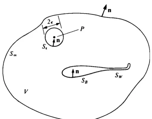
Fig 2.3: Nomenclature used to define the potential flow problem

From Katz(2001), Laplace's equation for the velocity potential must be solved for an arbitrary body with boundary SB enclosed in a volume V, with the outer boundary of the region we

consider S∞ , in Fig. 2.3. The boundary conditions in equation (2-18) and (2-19) apply to SB

and S∞. The normal vector we consider here is pointing out of the volume V. Now, the vector

appearing in the divergence theorem is replaced be the vector φ φ φ φ₁∇ ₂− ₂∇ ₁ , where ϕ1 and

ϕ2 are two scalar functions of position. This results in

(

)

(

2 2

)

1 2 2 1 d 1 2 2 1 d

T

V S

n S V

φ φ φ φ∇ − ∇ =

_∫

φ∇ φ φ− ∇ φ

∫

∫∫

∫

(2-29)

Equation (2-29) is one of Green's theorem. Here the surface integral is taken over all the boundaries S, including boundary of the infinite small sphere Sε.

S = SB + S∞ + Sε (2-30)

(16)

1 2 1

and

r

φ = φ =φ (2-31)

where ϕ is the potential of the flow we are interested in V, and r is the distance from a point P(x, y, z), as shown in Fig 2.3. We shall see later, ϕ1 is unbounded (1/r→∞) as P is

approached as r → 0 and is the potential of a source. In the case where the point is outside of V both ϕ1 and ϕ2 satisfy Laplace's equation and equation (2-29) becomes

1 1

d 0

S

T

n S r φ φ r

 _∇ _∇  ₌    − 

∫∫

(2-32)

We are more interested in the case when the point P is inside the volume V. The point P must now be excluded from the region of integration and it is surrounded by a small sphere of radius ε, then we create a simple connected region. So the potential ϕ satisfies Laplace's equation, when point P is outside of the sphere and in the remaining volume V. And equation (2-32) becomes

1 1

d 0

B

T

S S S

n S

r φ φ r

∞ + +  _∇ _∇  ₌   − 

∫∫

ε (2-33)

Let us consider about the integral over sphere Sε

1 1 1 1

d d d

T

S

T T

S S

n S n S n S

r φ φ r r φ φ r

    ₋    ∇ − ∇   = _ ∇ _  ∇        

∫∫

ε ε ε (2-34)

On the sphere surrounding point P, as ε→0 the first term in the first integral vanishes, and the second term becomes, more detail derive see Birk(2012).

0

1

lim d 4 ( )

T

S

n S P

r φ πφ →   ₌  ∇  _{ }  

∫∫

ε ε (2-35)

After we substitute equation (2-35) back to equation (2-34), the integral of the sphere surrounding point P yields

1 1

d

T

S

n S

r φ φ r

 _{∇ − ∇}  ₌        

∫∫

ε

-4πφ( )P (2-36)

And equation (2-33) becomes

1 1 1

( ) d

4

B

T

S S

P n S

r r φ φ φ π ∞ +   = _ ∇ ∇ _  − 

∫∫

(2-37)

Equation (2-37) gives the value of ϕ(P) at any point in the flow, within the volume V, in terms of the values of ϕ and ∂ϕ/∂n on the boundaries S.

Let us consider about the case that point P lies on the boundary SB. In order to exclude point

P from V, the integration is carried out only around the surrounding hemisphere with radius ε

and equation (2-37) becomes

1 1 1

( ) d

2

B

T

S

P n S

(17)

In our mathematical model the boundary condition on SB makes sure that SB is actually a

steam surface with no flow across it. However there may be also a flow inside the body SB.

The interior of the body Vinside becomes the fluid domain of interest. The interior fluid flow is

described by the potential ϕinside. We keep point P outside of Vinside and thus can reuse the

first case of exterior flow.

1 1

d 0

4 4

B

T

inside inside ins de

S

i

n S

r φ φ r

π π  _∇ _∇  ₌   −  

∫∫

(2-39)

Note that the boundary consists of body surface SB only. We replace the normal vector ninside

with the normal vector of the volume V.

inside

n = −n (2-40)

Then equation (2-39) becomes

1 1 d 0 4 4 B T inside in S

side n S

r φ φ r

π π  _∇ _∇  ₌  −  − _ 

∫∫

(2-41)

Now, we add equation (2-37) and (2-41), as we are going to consider both point outside of region V and inside the region V.

1 1 1

( ) 0 d

4 1 1 d 4 4 B B T S S T

inside insi e S

d

P n S

r r n S r r φ φ φ π φ φ π π ∞ + − −   + = _ ∇ ∇ _    _∇ _∇     − 

∫∫

(2-42)

We adjust for the integral on the body SB, then we have

1 1

( ) ( d

4 4 1 1 ) ( d ) 4 4 B T

inside insi e

T S

d

S

P n S

r r n S r r φ φ φ φ φ π π φ φ π π ∞   = _ ∇ − ∇ − ∇ _    − −  + _ ∇ ∇ _  

∫∫

(2-43)

We summaries the integral over S∞ as the so-called far field potential ϕ∞.

1 1 1

( ) d

4

T

S

P n S

r r φ φ φ π ∞ ∞ =  ∇ ∇   − 

∫∫

(2-44)

For our exterior flow problem with a body moving at a constant speed v∞ the far field

potential would be

) )

(P (u x v y w z P vT

φ_∞ =− _∞ + _∞ + _∞ = − _∞ (2-45)

The minus sign is a question definition. An observer on the body moving with speed v∞=( u∞,

(18)

1

( ) ( d

4

1

( d ( )

4 ) ) B B T inside T ins de S S i

P n S

r

n S P

r φ φ φ π φ φ φ π ∞   = _ ∇ − ∇ _      − _ − ∇_ __ +    

∫∫

(2-46)

We merge the normal vector with the nabla operator into the more common normal derivative.

( )T T

n n n φ φ φ ∂ ∇ = ∇ = ∂ (2-47) 1 1 4 4 T n

r n r

π π

_∇  ₌ ∂  

   

 _ _ _∂ _ _

  (2-48)

Let us substitute equation (2-47) and (2-48) into (2-46), then we have 1

( ) ( d

4 1 ) ( d ) 4 ) ( B B inside inside S S P S

r n n

S P n r φ φ φ π φ φ φ π ∞ ∂ ∂   = _ − _ ∂ ∂   ∂   − _ − _ __ +  ∂   

∫∫

(2-49)

From equation (2-49) we can define

inside n n φ φ σ ∂ ∂ − = −

∂ ∂ (2-50)

inside

µ φ φ

− = − (2-51)

In equation (2-50) is the unknown source strength and in equation (2-51) is the doublet strength.

We finally have the general solution of the exterior flow problem 1

( ) d

4

1

d ( )

4 B B S S P S r S P n r φ σ π µ φ π ∞   = _− _   ∂  −  − _ _ + ∂        

∫∫

(2-52)

The potential ϕ=ϕ(P) at a point P in the fluid domain can be represented by a combination

of a source distribution

4 r

σ π

₋ 

 

  and a doublet distribution

1 4 n r µ π ∂  −   

∂   over the body

surface.

(19)

We have a single integral equation for both source and doublet strength, thus we do not have a unique solution yet. A choice must be made how to combine or not to combine sources and doublets.

For out naval architecture problems it is more realistic to select ϕ=ϕi on SB thus eliminating the doublet distribution.

1

( ) d ( )

4

b

S

Rankine sources

p S p

r

φ σ φ

π ∞

−

 

= _ _ +

 

14243

∬

(2-53)

2.6 Derivation of Free Surface Boundary Condition

In this section, we are going to discuss the derivation of Kinematic Free Surface Boundary Condition(KFSBC), Dynamic Free Surface Boundary Condition(DFSBC) and the Combined Free Surface Boundary Condition (CFSBC).

We assume that the movement of the ship hull create a perturbation of the flow passing around and having a flat water surface.

φ = Φ +ϕ′ (2-54)

In equation (2-54), ϕis the free surface flow potential, Φ is the base potential and φ' is the perturbation potential.

H

η = +η′ (2-55)

In equation (2-55), η is the wave elevation of the free surface, H is the assumed wave surface and η' is a perturbation.

2.6.1 Kinematic Free Surface Boundary Condition

As we added perturbation in the flow potential and wave elevation, let us substitute equation (2-54) and (2-55) into kinematic free surface boundary condition (2-26)

( _x ϕ_x′)(H_x η′_x) ( _y ϕ_y′)(H_y η′_y) ( _z ϕ_z′) 0

− Φ + + − Φ + + + Φ + = (2-56)

After the multiplication of the first two terms, we have

( )

( ) ( ) 0

x x x x x x x x

y y y y y y y y z z

H H

η ϕ ϕ η

η ϕ ϕ η ϕ

′ ′ ′ ′

− Φ + Φ + +

′ ′ ′ ′ ′

− Φ + Φ + + + Φ + = (2-57)

(20)

0

x x x x x x

y y y y y y z z

H H

η ϕ

η ϕ ϕ

′ ′

Φ + Φ +

′ ′ ′

+Φ + Φ + − Φ − = (2-58)

We combine the common terms

( ) ( )

0

x x x y y y

x x y y z z

H H

η η

ϕ ϕ ϕ

′ ′

Φ + + Φ +

′ ′ ′

+ + − Φ − = (2-59)

Furthermore, the first two terms contain the partial derivative of equation (2-55) yields

0

xηx yηy Hxϕx′ Hyϕ′y z ϕz′

Φ + Φ + + − Φ − = (2-60)

Equation (2-60) is the linearised kinematic free surface boundary condition.

2.6.2 Dynamic Free Surface Boundary Condition

We substitute equation (2-54) into dynamic free surface boundary condition (2-28) yields

2 2 2 2

1

[ ( ) ( ) ( ) ] 0

2 ub − Φ +x ϕx′ − Φ +y ϕ′y − Φ +z ϕ′z −gη= (2-61)

After the calculation of the quadratic equation inside the bracket, equation (2-61) becomes

2 2 2 2 2

2 2

1

[ ( 2 ) ( 2 )

2

( 2 )] 0

b x x x x y y y y

z z z z

u

g

ϕ ϕ ϕ ϕ

ϕ ϕ η

′ ′ ′ ′

− Φ + Φ + − Φ + Φ +

′ ′

− Φ + Φ + − =

(2-62)

Neglect the small terms, we have

2 2 2 2

1

( 2 2 2 )

2g ub x y z x x y y z z

η= − Φ − Φ − Φ − Φ ϕ′− Φ ϕ′ − Φϕ′ (2-63)

Equation (2-63) is the linearised dynamic free surface boundary condition.

2.6.3 Combined Free Surface Boundary Condition

We must be careful when we are doing the substitution of the wave elevation η from the dynamic condition into the kinematic condition, since η is a function of (x,y) alone, while the right hand side of the dynamic condition in principle is a function F(x,y,z). Consequently

( ) ( )

x x y y xFx x xFz yFy y yFz xFx yFy zFz

φ η +φ η = φ +φ η + φ +φ η =φ +φ +φ (2-64)

in which we have used the kinematic condition. However, in our implementation the partial derivatives of F are defined as differences between values in field points which are on the free surface, so the Fz contribution is inherently taken into account.

(21)

2 2 2 2

2 2 2 2 1

( 2 2 2 )

2 1

( 2 2 2 )

2

0

b x y z x x y y z z

x

b x y z x x y y z z

y

x x y y z z

u g x u g y H H ϕ ϕ ϕ ϕ ϕ ϕ ϕ ϕ ϕ  _′ _′ _′  ∂_ − Φ − Φ − Φ − Φ − Φ − Φ _   Φ ∂  _′ _′ _′  ∂_ − Φ − Φ − Φ − Φ − Φ − Φ _   +Φ ∂ ′ ′ ′ + + − Φ − = (2-65)

Let us do the partial derivative in each term inside the bracket, then we have

2 2 2 2 2 2 2 2 2 1 ( ) 2 2 2 2 1 ( ) 2

y y y

x z x x z z

x

y y y

x z x x z z

y

x

g x x x x x x

g y y y y y y

H ϕ ϕ ϕ ϕ ϕ ϕ ϕ ′ ∂Φ ′ ∂ Φ ′ ∂Φ ∂Φ ∂ Φ ∂ Φ Φ − − − − − − ∂ ∂ ∂ ∂ ∂ ∂ ′ ∂Φ ′ ∂ Φ ′ ∂Φ ∂Φ ∂ Φ ∂ Φ +                 Φ − − − − − − ∂ ∂ ∂ ∂ ∂ ∂ ′

+ _x+ϕ′_yH_y− Φ −_z ϕ_z′ =0

(2-66)

Extract the minus sign outside the bracket, we have

2 2 2

2 2 2 1

( 2 2 2 )

2 1

( 2 2 2 )

2

0

x x y z x x y y z z

y x y z x x y y z z

x x y y z z

g x g y H H ϕ ϕ ϕ ϕ ϕ ϕ ϕ ϕ ϕ ∂ _′ _′ _′ − Φ Φ + Φ + Φ + Φ + Φ + Φ ∂ ∂ _′ _′ _′ − Φ Φ + Φ + Φ + Φ + Φ + Φ ∂ ′ ′ ′ + + − Φ − = (2-67)

After we combine the common terms, equation (2-67) becomes

2 2 2 1

( )( 2 2 2 )

2

0

x y x y z x x y y z z

x x y y z z

g x y

H H ϕ ϕ ϕ ϕ ϕ ϕ ∂ ∂ ′ ′ ′ − Φ + Φ Φ + Φ + Φ + Φ + Φ + Φ ∂ ∂ ′ ′ ′ + + − Φ − = (2-68)

Again let us do the partial derivative for each terms inside the bracket, then we have

1

[( 2 2 2 2 2

2g x x xx x y yx x z zx x xxϕx′ x xϕxx′

− Φ Φ Φ + Φ Φ Φ + Φ Φ Φ + Φ Φ + Φ Φ

2 2 2 2 )

( 2 2 2 2 2

2 2 2 2 )]

0

x yx y x y yx x zx z x z zx

y x xy y y yy y z zy y xy x y x xy

y yy y y y yy y zy z y z zy

xHx yHy z z

(22)

Extract 2 out of the bracket

2 2

2

1 [(

)

(

)]

0

x xx x y yx x z zx x xx x x xx

x y xy y yy y z zy y xy x x y xy

y yy y y yy y zy z y z zy

x x y y z z

g

H H

ϕ ϕ

ϕ ϕ ϕ ϕ

ϕ ϕ

ϕ ϕ ϕ ϕ

ϕ ϕ ϕ

′ ′

− Φ Φ + Φ Φ Φ + Φ Φ Φ + Φ Φ + Φ

′ ′ ′ ′

+Φ Φ + Φ Φ + Φ Φ + Φ Φ

′ ′

+ Φ Φ Φ + Φ Φ + Φ Φ Φ + Φ Φ + Φ Φ

′ ′ ′ ′

+Φ Φ + Φ + Φ Φ + Φ Φ

′ ′ ′

+ + − Φ − =

(2-70)

The last step, we time gravity acceleration to both side of equation (2-70), finally we have the combined free surface condition

2 2

2

(

)

0

x x y y z z

g H g H g g

ϕ ϕ

ϕ ϕ ϕ ϕ

ϕ ϕ

ϕ ϕ ϕ ϕ

ϕ ϕ ϕ

′ ′

Φ Φ + Φ Φ Φ + Φ Φ Φ + Φ Φ + Φ

′ ′ ′ ′

+Φ Φ + Φ Φ + Φ Φ + Φ Φ

′ ′

+Φ Φ Φ + Φ Φ + Φ Φ Φ + Φ Φ + Φ Φ

′ ′ ′ ′

+Φ Φ + Φ + Φ Φ + Φ Φ

′ ′ ′

− − + Φ + =

(2-71)

(23)

Chapter 3 The nonlinear ship wave solution

3.1 Basic Integral Equation

In this section, we will transform the boundary equation into integral form. In order to solve from the potential problem, we will use equation (2-53) to compute the potential in the region. The equations will have to satisfy all the boundary equations we derived in the last section. The following is the build up process of the integral equation of the boundary conditions.

We use the Newmann-Kelvin condition as the initial condition of the problem. The condition define the initial velocity distribution and the initial wave height.

0

bx

u −

 

 

Φ =  

 

 

(3-1)

H=0 (3-2)

The ship velocity is ub, as the ship is traveling towards the positive x-direction, the flow potential in x-direction become -ubx. The initial wave height distribution is zero.

3.1.1 The Integral equation on ship hull

The ship hull boundary condition is similar to the case we discuss in section 2.5. It is consider to a deeply submerged body and no flow can go through the body. Recall equation (2-18).

0

n

φ ∂

∂ = (3-3)

The normal vector in equation (3-3) is defined to point into the body. Then we can rewrite the equation

0

T

n ∇ =φ (3-4)

(24)

1

0

0 '

b

T T

b

n n

u

n u

ϕ

    =      

∇ = (3-5)

Then the source strength distribution ϕ which provides us with the perturbation potential φ'.

1

( ) ( ) d

4 ( , ) q

S

p q S

r P q

ϕ σ

π

 − 

′ = _ _

 

∬

(3-6)

Note that, point q is the field in the region we are considering and point P is all the points on the ship hull.

Substituting equation (3-6) into equation (3-5), we have

( ) 1

1

( ) d

4 ( , )

T

P q b

S

n q S

r P q n u

σ

π



=  −

∇ _ _

 

∬

(3-7)

The normal vector and the gradient are taken with respect to the point P. The integration is over all points q. Since we also have to satisfy a free surface condition we have to distribute sources on the ship hull body surface as well as the free surface.

The integration domain then includes the ship hull body surface SB and the free surface SF.

For a point P on the surface S we have to consider point p is superimpose with point P for the region. As we have discussed in section 2.5, this special case will become the integral over

the hull sphere Sε, as equation (2-38), then yields

δP. Equation (3-7) becomes

( ) 1

1 1

(P) ( ) d

2 4 ( , )

T

P q b

S

n q S

r P q nu

σ σ

π

 − 

− + ∇ _ _

  =

∬

(3-8)

Equation (3-8) is the integral equation of the ship hull.

3.1.2 The Integral Equation on Free Surface

In comparison to the boundary value problem of a deeply submerged body difference come from the free surface and the resulting wave body interaction. Again we will follow an approach which attempts a solution using a surface distribution of Rankine sources, equation (3-6). This is by far the most common approach today. However, more complicated singularities have been used, for example, Havelock-source which already satisfy the Newmann-Kelvin linearization thus eliminating the need to distribute sources on the free surface. However these approaches are difficult to extend to nonlinear free surface conditions.

(25)

φ = Φ +ϕ′ (3-9)

We substitute equation (3-6) into equation (3-8). The total velocity potential at a point P = (x, y, z) then becomes

1

( ) ( ) ( ) d

4 ( , ) q

S

P P q S

r P q

φ σ

π

 − 

= Φ + _ _

 

∬

(3-10)

On the free surface we have to satisfy the combined free surface boundary condition, we recall equation (2-70)

2 2

2

(

)

0

x x y y z z

g H g H g g

ϕ ϕ

ϕ ϕ ϕ ϕ

ϕ ϕ

ϕ ϕ ϕ ϕ

ϕ ϕ ϕ

′ ′

Φ Φ + Φ Φ Φ + Φ Φ Φ + Φ Φ + Φ

′ ′ ′ ′

+Φ Φ + Φ Φ + Φ Φ + Φ Φ

′ ′

+Φ Φ Φ + Φ Φ + Φ Φ Φ + Φ Φ + Φ Φ

′ ′ ′ ′

+Φ Φ + Φ + Φ Φ + Φ Φ

′ ′ ′

− − + Φ + =

(26)

(27)

Put forward the common factor σ(q) and move the parts that do not have σ(q) to the right hand side of the equation, we have:

(

x xx x y yx x z zx x y xy y yy y z zy z

)

q b F S q b F S y q b F S x q b F S z y q b F S zy y q b F S y q b F S yy y q b F S y x q b F S xy y q b F S z x q b F S zx x q b F S y x q b F S yx x q b F S x q b F S xx x g q S q p r z S g S q p r y S gH S q p r x S gH S q p r y z S S q p r z S S q p r y S S q p r y S S q p r y x S S q p r x S S q p r x z S S q p r z S S q p r x y S S q p r y S S q p r x S S q p r x S Φ + Φ Φ Φ + Φ Φ + Φ Φ Φ + Φ Φ Φ + Φ Φ Φ + Φ Φ − •       − ∂ ∂ + +       − ∂ ∂ + −       − ∂ ∂ + −       − ∂ ∂ ∂ + Φ Φ +       − ∂ ∂ + Φ Φ +       − ∂ ∂ + Φ +       − ∂ ∂ + Φ Φ +       − ∂ ∂ ∂ + Φ Φ +       − ∂ ∂ + Φ Φ +       − ∂ ∂ ∂ + Φ Φ +       − ∂ ∂ + Φ Φ +       − ∂ ∂ ∂ + Φ Φ +       − ∂ ∂ + Φ Φ +       − ∂ ∂ + Φ +       − ∂ ∂ + Φ Φ

∫∫

2 2 2 2 2 2 2 2 2 2 2 2 = ) ( d ) , ( 4 1 d ) , ( 4 1 d ) , ( 4 1 d ) , ( 4 1 d ) , ( 4 1 d ) , ( 4 1 d ) , ( 4 1 d ) , ( 4 1 d ) , ( 4 1 d ) , ( 4 1 d ) , ( 4 1 d ) , ( 4 1 d ) , ( 4 1 d ) , ( 4 1 d ) , ( 4 1 σ π π π π π π π π π π π π π π π (3-13)

Normally, we would again have to discuss the case P=q where the field point P approaches the source at q. However, it is common to take a different path for the free surface: we will desingularize the free surface condition. We remove the sources form the boundary z=0 and place them slight above it, this is so called raised panel method. The sources are not placed on SF but on a raised, parallel surface S'F. We have to satisfy the free surface boundary

condition on z=0, thus P on SF and consequently P is never equal to q. Of course now the

integration has to be performed over the raised surface S'F.

3.2 Discretization of the Integral equation

3.2.1 Discretization of the ship hull

The integral equation (3-8) are to be satisfied everywhere on the ship hull body surface SB

which consists of an infinite number of points q. In addition, the unknowns source strength ϕ

is part of the integrand which makes a solution difficult.

(28)

In order to remove ϕ from the integral we have to know or assume something about how the quantity in distributed locally. Since it is impossible to guess for the complete surface we subdivide the body surface SB into small parts, so called panels.

1

1 1

( ) d ( ) d

4 4

B j

N

j

P P

S S

q S q S

n r n r

δ δ

σ σ

δ π = δ π

₋  ₌ ₋ 

   

   

∫∫

∑

∫∫

(3-14)

np is the vector pointing from point P to panel center point q.

Note, this transformation itself is exact, as long as the collection of all surface panels Sj

represent the true ship hull body surface.

The simplest approach to extract ϕ from the integral and by far the most widely used approach is to assume that ϕ is constant over a panel Sj and takes the value at its center qj.

This will result is a so called zero order panel method. Other names are constant strength panel method. The integral equation now reads

( ) 1

1 1

( ) ( d

2 ) 4 ( , )

j

S N

T

j q P

j P

P q S n v

n r P q

δ

σ σ

δ π ∞

=

 

− + _− _ =

 

∫

∑

_∫

(3-15)

It is obvious that for N→∞ this will converge to the original integral equation. This equation still has to be satisfied at an infinite number of points P. Now we have to restrict the integral equation to a finite number of points.

Instead of satisfying (3-14) on infinite points in the space, we restrict ourselves to a finite number of points. In another words, we have finite number of panel centers Pi.

( ) 1

1 1

( ) ( d

2 4 ( , )

) ( ) ( )

1, 2, ,

j

N

T T

i j i q i

j S i

P q n S n v

r P

i

P q P

N

σ σ

π ∞

=

 

− + _− _ =

 

∑

_∫∫

L

(3-16)

We introduce some abbreviations:

( )Pi i

σ =σ (3-17)

(q_j) ( )P_j _j

σ =σ =σ (3-18)

( )i i

n P =n (3-19)

) (

T

i i

(29)

( )

1 d

4 ( , )

j

i q ij

i S

n S

r P q D

π

 

∇ −_

  =

∫∫

(3-21)

Then equation (3-16) becomes:

1

1, 2

2 , ,

N

i j ij i

j i b D N σ σ = =

− +

∑

= L (3-22)

3.2.2 Discretization of the free surface

Equation (3-8) and (3-12) form a system of two coupled integral equations, to be satisfied at every point P on the body and the calm water surface.

To derive algebraic equations which we can solve on a computer we will select NB points Pi( i

= 1,2,...,NB) on the body surface and NF points Pi( i = NB+1, NB+2, ..., NB+NF) on the free

surface where we will check the boundary conditions. This yields

(

x xx x y yx x z zx x y xy y yy y z zy z

)

q i b F S q i b F S y q i b F S x q i b F S z y q i b F S zy y q i b F S y q i b F S yy y q i b F S y x q i b F S xy y q i b F S z x q i b F S zx x q i b F S y x q i b F S yx x q i b F S x q i b F S xx x g q S q P r z S g S q P r y S gH S q P r x S gH S q P r y z S S q P r z S S q P r y S S q P r y S S q P r y x S S q P r x S S q P r x z S S q P r z S S q P r x y S S q P r y S S q P r x S S q P r x S Φ + Φ Φ Φ + Φ Φ + Φ Φ Φ + Φ Φ Φ + Φ Φ Φ + Φ Φ − •       − ∂ ∂ + +       − ∂ ∂ + −       − ∂ ∂ + −       − ∂ ∂ ∂ + Φ Φ +       − ∂ ∂ + Φ Φ +       − ∂ ∂ + Φ +       − ∂ ∂ + Φ Φ +       − ∂ ∂ ∂ + Φ Φ +       − ∂ ∂ + Φ Φ +       − ∂ ∂ ∂ + Φ Φ +       − ∂ ∂ + Φ Φ +       − ∂ ∂ ∂ + Φ Φ +       − ∂ ∂ + Φ Φ +       − ∂ ∂ + Φ +       − ∂ ∂ + Φ Φ

∫∫

2 2 2 2 2 2 2 2 2 2 2 2 = ) ( d ) , ( 4 1 d ) , ( 4 1 d ) , ( 4 1 d ) , ( 4 1 d ) , ( 4 1 d ) , ( 4 1 d ) , ( 4 1 d ) , ( 4 1 d ) , ( 4 1 d ) , ( 4 1 d ) , ( 4 1 d ) , ( 4 1 d ) , ( 4 1 d ) , ( 4 1 d ) , ( 4 1 σ π π π π π π π π π π π π π π π (3-23)

Like for the submerged body we have to extract the unknown sources strength ϕ from the integrals. We will discretize the raised surface S'F and the ship hull body surface SB into

(30)

small panels For body and raised free surface we define as many panels as we have field points, body surface NB panels and free surface NF panels.

All integrals will be converted into sums of integrals over panels Sj. We assume the source

strength to be constant on small panels Sj. We assume ϕ to be constant over an individual Sj

with strength ϕ(qj). Note that qj is the center of panel Sj.

Then equation (3-22) turns into

2 2 2 1 1 2 1 1 1 1 d d

4 ( , ) 4 ( , )

1 1

d d

4 ( , ) 4 ( , )

1 4

B F B F

N N N N

x xx q x q

i i

j j

S_F _b S_F _b

N N N N

x yx q x y q

i i

j j

S_F _b S_F _b

x zx

S_F _b

S S

x r P q x r P q

S S

y r P q y x r P q

S S z S π π π π + + = = + + = =     ∂ − ∂ − Φ Φ _ _ +Φ _ _ ∂ _ _ ∂ _ _ + +     ∂ − ∂ − +Φ Φ _ _ +Φ Φ _ _ ∂ _ _ ∂ ∂ _ _ + + ∂ − +Φ Φ ∂ +

∑

_∫∫

∑

_∫∫

∑

∫∫

∑

∫∫

2 1 1 2 1 1 1 d d

( , ) 4 ( , )

1 1

d d

4 ( , ) 4 ( , )

1 d 4 ( , )

B F B F

N N N N

q x z q

i i

j j _S

F b

N N N N

y xy q x y q

i i

j _S j _S

F b F b

y yy

i S_F _b

S S

r P q _S z x r P q

S S

x r P q x y r P q

S S

S y r P q S π π π π π + + = = + + = =   _{+Φ Φ} ∂  −    _{∂ ∂}     ₊       ∂ − ∂ − +Φ Φ _ _ +Φ Φ _ _ ∂ _ _ ∂ ∂ _ _ + +   ∂ − +Φ Φ _ _ ∂   +

∑

∑ ∫∫

∑

∫∫

∑

∫∫

2 2

2 1 1 2 1 1 1 1 d 4 ( , )

1 1

d d

4 ( , ) 4 ( , )

1 d 4 ( , )

B F B F

B F

N N N N

q y q

i

j j _S

F b

N N N N

y zy q y z q

i i

j _S j _S

F b F b

N N

x q y

i

j _S _S

F b F

S y r P q S

S S

z r P q z y r P q

S S

gH S gH

x r P q

S S π π π π + + = = + + = = + =   ∂ − +Φ _ _ ∂   +     ∂ − ∂ − +Φ Φ _ _ +Φ Φ _ _ ∂ _ _ ∂ ∂ _ _ + +   ∂ − − _ _ − ∂   + +

∑

∑ ∫∫

∑

∫∫

∑

∫∫

∑ ∫∫

∫∫

1 1 1 2 2 ( ) 1 d 4 ( , ) 1

d 4 ( , )

B F B F B F N N j N N q i j b N N q i j

S_F _b

x xx x y yx x z zx x y xy y yy z

j

y zy

q

S y r P q

g S

z r P q S g σ π π + = + = + =                              _•                _ _  ∂ −  _ _   _{∂ } _     _∂_ ₋ _  + _ _  ∂  ₊ _ _    =− Φ Φ +Φ Φ Φ +Φ ΦΦ +Φ Φ Φ +Φ Φ +Φ ΦΦ + Φ

∑

∑ ∫∫

(

z

)

(3-24)

As for the submerged body we have reduced the integrals to coefficients which only depend on geometric information we know.

A Nonlinear Ship Wave Solution Method

ScholarWorks@UNO

ScholarWorks@UNO

A Nonlinear Ship Wave Solution Method

A Nonlinear Ship Wave Solution Method

A Nonlinear Ship Wave Solution Method

Contents

List of Figures

Abstract

Chapter 1

Introduction

Chapter 2

Theoretical Background

2.1

Limitation of the problem

2.2

Basic Equation

∫∫∫

∫∫

∫∫∫

2.3

The Laplace Equation

2.4

The Boundary Condition

2.4.1

Ship Hull Boundary Condition

2.4.2

Free Surface Boundary Condition

(

)

2.5

General solution of exterior flow problem

(

)

(

)

∫

∫

∫∫

∫

∫∫

∫∫

∫∫

∫∫

∫∫

∫∫

∫∫

∫∫

∫∫

∫∫

∫∫

∫∫

∫∫

∫∫

∫∫

∫∫

∫∫

∫∫

∫∫

∫∫

∫∫

∬

2.6

Derivation of Free Surface Boundary Condition

2.6.1

Kinematic Free Surface Boundary Condition

2.6.2

Dynamic Free Surface Boundary Condition

2.6.3

Combined Free Surface Boundary Condition

Chapter 3

The nonlinear ship wave solution

3.1

Basic Integral Equation

3.1.1

The Integral equation on ship hull

∬

∬

∬

3.1.2

_∫

_∫

_∫∫

_∫∫

_∫∫