MASSIVELY PARALLEL ALGORITHM FOR SOLVING THE EIKONAL EQUATION ON MULTIPLE ACCELERATOR PLATFORMS

(1)

THE EIKONAL EQUATION ON MULTIPLE

ACCELERATOR PLATFORMS

by Anup Shrestha

A thesis

submitted in partial fulfillment of the requirements for the degree of Master of Science in Computer Science

Boise State University

(2)

(3)

DEFENSE COMMITTEE AND FINAL READING APPROVALS

of the thesis submitted by

Anup Shrestha

Thesis Title: Massively Parallel Algorithm for Solving the Eikonal Equation on Multiple Accelerator Platforms

Date of Final Oral Examination: 14 October 2016

The following individuals read and discussed the thesis submitted by student Anup Shrestha, and they evaluated his presentation and response to questions during the final oral examination. They found that the student passed the final oral examination. Elena A. Sherman, Ph.D. Chair, Supervisory Committee

˙Inan¸c S¸enocak, Ph.D. Co-Chair, Supervisory Committee

Steven M. Cutchin, Ph.D. Member, Supervisory Committee

(4)

I would like to thank my advisors Dr. Elena Sherman and Dr. ˙Inan¸c S¸enocak for their continuous guidance and support throughout the course of this Master’s thesis. I would also like to thank Dr. Steven Cutchin for serving on my thesis supervisory committee. Many thanks to Boise State University and Jason Cook in particular for help with the local computing infrastructure and installation of various tools and libraries. I would also like to thank my colleagues Rey DeLeon and Micah Sandusky, from the High Performance Simulation Laboratory for Thermo-Fluids, for their help and willingness to answer my questions. Finally, I would like to thank my family for their continued support.

I am grateful for the funding during my graduate studies, provided by the National Science Foundation under grants number 1229709 and 1440638.

(5)

The research presented in this thesis investigates parallel implementations of the Fast Sweeping Method (FSM) for Graphics Processing Unit (GPU)-based compu-tational platforms and proposes a new parallel algorithm for distributed computing platforms with accelerators. Hardware accelerators such as GPUs and co-processors have emerged as general-purpose processors in today’s high performance computing (HPC) platforms, thereby increasing platforms’ performance capabilities. This trend has allowed greater parallelism and substantial acceleration of scientific simulation software. In order to leverage the power of new HPC platforms, scientific applications must be written in specific lower-level programming languages, which used to be platform specific. Newer programming models such as OpenACC simplifies imple-mentation and assures portability of applications to run across GPUs from different vendors and multi-core processors.

The distance field is a representation of a surface geometry or shape required by many algorithms within the areas of computer graphics, visualization, computational fluid dynamics and more. It can be calculated by solving the eikonal equation using the FSM. The parallel FSMs explored in this thesis have not been implemented on GPU platforms and do not scale to a large problem size. This thesis addresses this problem by designing a parallel algorithm that utilizes a domain decomposition strat-egy for multi-accelerated distributed platforms. The proposed algorithm applies first coarse grain parallelism using MPI to distribute subdomains across multiple nodes and then fine grain parallelism to optimize performance by utilizing accelerators. The results of the parallel implementations of FSM for GPU-based platforms showed speedup greater than 20× compared to the serial version for some problems and the

(6)

solve large memory problems with comparable runtime efficiency.

(7)

ACKNOWLEDGMENTS . . . iv

ABSTRACT . . . v

LIST OF TABLES . . . xi

LIST OF FIGURES . . . xii

LIST OF ABBREVIATIONS . . . xv

1 Introduction . . . 1

1.1 Problem Context . . . 1

1.2 Review of Processor Hardware and Accelerators . . . 2

1.3 Software Engineering for Scientific Computing . . . 4

1.4 Thesis Statement . . . 6

1.4.1 Objectives . . . 6

1.4.2 Procedures . . . 7

2 Background . . . 9

2.1 Simulation Problem: Signed Distance Field . . . 9

2.1.1 Calculating Signed Distance Field . . . 10

2.1.2 The Eikonal Equation . . . 10

2.2 Solution Algorithms . . . 13

2.2.1 Dijkstra’s Algorithm . . . 13

2.2.2 Fast Marching Method (FMM) . . . 14

(8)

2.3 Parallel Algorithms for FSM . . . 17

2.3.1 Parallel Algorithm of Zhao . . . 18

2.3.2 Parallel Algorithm of Detrixhe et al. . . 20

2.3.3 Hybrid Parallel Algorithm . . . 22

2.4 Hardware Accelerators . . . 24

2.4.1 Graphics Processing Unit (GPU) . . . 25

2.4.2 Intel Xeon Phi Co-processor . . . 27

2.5 Programming Models . . . 28

2.5.1 Compute Unified Device Architecture (CUDA) . . . 29

2.5.2 Open Accelerators (OpenACC) . . . 32

2.5.3 Message Passing Interface (MPI) . . . 34

2.6 Parallel FSM Implementations . . . 36

2.6.1 Common Implementation Details . . . 36

2.6.2 MPI Implementation of Zhao’s Method . . . 37

2.6.3 CUDA Implementation of Detrixhe et al.’s Method . . . 38

2.6.4 OpenACC Implementation of Detrixhe et al.’s Method . . . 41

2.6.5 MPI/CUDA Implementation of Hybrid Parallel FSM . . . 42

2.6.6 MPI/OpenACC Implementation of Hybrid Parallel FSM . . . 44

3 Parallel FSM Algorithm for Distributed Platforms with Accelerators47 3.1 Method . . . 47

3.1.1 Domain Decomposition . . . 48

3.1.2 Algorithm and Implementation . . . 50

3.2 Network Common Data Form (NetCDF) . . . 56

3.2.1 File Format . . . 56

(9)

4.1 Simulation Problem: Complex Geometry . . . 58

4.2 Benchmark Serial FSM (Algorithm 1) . . . 59

4.3 Zhao’s Parallel FSM (Algorithm 2) . . . 60

4.4 Detrixhe et al.’s Parallel FSM (Algorithm 3) . . . 63

4.5 Hybrid (Zhao and Detrixhe et al.) Parallel FSM (Algorithm 4) . . . 65

4.6 Parallel FSM Algorithm for Distributed Platforms with Accelerators (Algorithm 5) . . . 66

4.7 Results Summary . . . 70

4.8 Threats to Validity . . . 70

5 Conclusions . . . 72

5.1 Summary . . . 72

5.2 Future Work . . . 73

REFERENCES . . . 75

APPENDIX A Coding Style Guide . . . 78

A.1 Program Organization . . . 79

A.1.1 README File . . . 80

A.1.2 Header Files . . . 81

A.1.3 Source Files . . . 83

A.2 Recommended C Coding Style and Conventions . . . 85

A.2.1 Naming . . . 85

A.2.2 Indentation . . . 87

A.2.3 Braces . . . 87

A.2.4 Spaces . . . 88

A.2.5 Commenting . . . 89

(10)

APPENDIX B NetCDF File Format . . . 93

APPENDIX C Method that Solves the Eikonal Equation . . . 95

APPENDIX D Timing Code Snippets . . . 98

(11)

2.1 Platforms supported by OpenACC compilers [22]. . . 33

4.1 Benchmark runtime of the serial implementation of FSM. . . 59 4.2 Runtime for hybrid parallel Algorithm 5 w/o OpenACC directives. . . 68 4.3 Runtime for hybrid parallel Algorithm 5 with OpenACC directives. . . . 68

A.1 Recommended Naming Convention . . . 85

(12)

1.1 NVIDIA GPU performance trend from 2000 to 2017 A.D. [17] . . . 4

2.1 Signed distance calculation for a point on 2D grid with interfaceφ . . . . 9 2.2 Distance field visualization of the Stanford Dragon (left) and the

Stan-ford Bunny (right) . . . 10 2.3 2D shape with inside and outside regions separated by an interface . . . . 11 2.4 Dijkstra’s algorithm finding the shortest path (shown in red). Actual

shortest distance is the diagonal (shown in blue). . . 14 2.5 The first sweep ordering of FSM for a hypothetical distance function

calculation from a source point (center) [7] . . . 18 2.6 Parallel FSM of Zhao in 2D . . . 19 2.7 Cuthill-McKee ordering of nodes into different levels [7] in two

dimen-sions (left) and three dimendimen-sions (right) . . . 21 2.8 CPU and GPU fundamental architecture design. [19] . . . 26 2.9 A schematic of the CPU/GPU execution [21]. . . 27 2.10 CUDA Thread Hierarchy Model (left), CUDA Memory Hierarchy Model

(right) [19]. . . 30

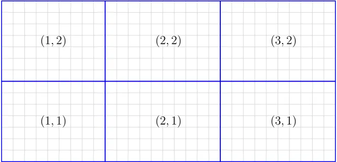
3.1 A 3×2 decomposition of the domain. Each block is labeled by a two dimensional coordinate system starting at index 1. . . 48 3.2 Cuthill McKee ordering of the decomposed blocks. The sum of the

coordinates and the colors represent the levels of the Cuthill McKee ordering. . . 49

(13)

blocks represents that each block is managed by a different MPI process that might be running on a separate node with enough memory resources.52 3.4 The first sweep iteration of FSM by the block in level two of the Cuthill

McKee ordering. . . 52 3.5 Exchange of ghost cell values from level two block on to level three blocks.53 3.6 Continuation of the first sweep iteration of FSM on to the next next

level. The two blocks on level three are executed simultaneously. . . 53

4.1 Surface representation of a complex terrain. The two slices depict the visualization of the distance field from a complex terrain. . . 58 4.2 Acceleration of FSM calculation on a single node with multiple cores

using MPI implementation of Algorithm 2. Speedup relative to se-rial implementation is plotted for various physical domain sizes and different number of processes. . . 60 4.3 Acceleration of FSM calculation on multiple nodes (2

processes/n-ode) with multiple cores using MPI implementation of Algorithm 2. Speedup relative to serial implementation is plotted for various physical domain sizes and different number of processes. . . 61 4.4 Percent of time spent in computation and communication in a single

node (left) and multi-node (right) environment by Algorithm 2 imple-mented using MPI. . . 62 4.5 Runtime of FSM calculation on GPU using CUDA and OpenACC

implementation of Algorithm 3. The runtime of CUDA and OpenACC implementation is plotted for various physical domain sizes. . . 63

(14)

implementation of Algorithm 3. GPU speedup relative to serial CPU implementation is plotted for various physical domain sizes. The CUDA implementation results in higher speedup than OpenACC implementation.64 4.7 Acceleration of FSM calculation on a single node multi-core

proces-sor, single GPU using MPI/CUDA implementation of Algorithm 4. Speedup relative to serial implementation is plotted for various physical

domain sizes and different number of processes. . . 66

4.8 Acceleration of FSM calculation on a single node multi-core processor, single GPU using MPI/OpenACC implementation of Algorithm 4. Speedup relative to serial implementation is plotted for various physical domain sizes and different number of processes. . . 67

4.9 Result of increasing the number of processes by changing the decom-position parameter using Algorithm 5 w/o OpenACC directives. . . 69

4.10 Result of increasing the number of processes by changing the decom-position parameter using Algorithm 5 with OpenACC directives. . . 69

A.1 Program Organization Schema . . . 80

A.2 README file template . . . 82

A.3 C header file template . . . 84

A.4 C source file template . . . 86

A.5 C function template . . . 91

(15)

AMD – Advanced Micro Devices, Inc.

API– Application Programming Interface

ASCII– American Standard Code for Information Interchange

CPU – Central Processing Unit

CUDA – Compute Unified Device Architecture

DRAM – Dynamic Random Access Memory

FLOPS – Floating Point Operations per Second

FMM – Fast Marching Method

FSM – Fast Sweeping Method

GPGPU – General-Purpose computation on Graphics Processing Units

GPU – Graphics Processing Unit

HDF5 – Hierarchical Data Format 5

HPC – High Performance Computing

I/O – Input/Output

MIC – Many Integrated Cores

MIMD – Multiple Instruction Multiple Data

MISD – Multiple Instruction Single Data

MPI – Message Passing Interface

NetCDF– Network Common Data Formt

(16)

OpenCL – Open Computing Language

OpenGL – Open Graphics Library

OpenMP – Open Multi Processing

PCI – Peripheral Component Interconnect

POSIX – Portable Operating System Interface

SIMD – Single Instruction Multiple Data

SISD – Single Instruction Single Data

SM – Streaming Multiprocessors

XDR – eXternal Data Representation

(17)

CHAPTER 1 INTRODUCTION

1.1 Problem Context

Imagine a robot that wants to make its way from point A to point B in an environment with static and moving objects. For the robot to reach its destination efficiently and safely, it needs to find a collision free shortest path from its current location to the destination. To avoid collision the robot needs to know the distance between it and the surrounding objects. Using geometric primitives to calculate the distance between the robot and other objects each time it moves is very inefficient. Instead collision detection/avoidance algorithms utilize the concept of a distance field. Distance field is a gridded structure where each cell in the grid is a point in space, value of which represents the shortest distance between that point and the boundary of the closest object. Distance field can be signed or unsigned. Signed distance fields store the sign to distinguish whether the query point lies inside or outside of an object. The advantage of using distance field is that it can approximate the distance from any arbitrary point to the nearest object in O(1) time, independent of the geometric complexity of the object [3].

(18)

methods still remain a topic of research. In general, speedup is achieved either by developing an algorithm with better performance or by executing the existing code on a machine with high processing power. In the last decade, the processing power of a single CPU has stalled and designers have shifted to a multi-core architecture where multiple CPUs are integrated into single circuit die. The idea here is to use parallelism by which higher data throughput may be achieved with lower voltage and frequency [24]. This means that executing the existing code on multi-core architecture results in no performance increase. Therefore, developers could no longer rely on hardware upgrades to increase the performance. Instead parallel algorithms are the key on taking advantage of the multi-core architecture. Further increase in performance could be achieved by leveraging the computational power of advanced hardware platforms such as the Graphical Processing Unit (GPU) or Intel Xeon Phi co-processor. They have adopted the multi-core architecture since their inception and can offer much higher throughput and combined processing power than the multi-core CPUs.

Orthogonal to performance increase, computation of distance field faces the issue of memory limitation when a domain is either large or has been refined into a finer grid for a high resolution. If the memory requirements of the domain exceeds the available system memory then the calculation cannot be performed. The solution is to store the grid using a file format that supports parallel I/O. With parallel I/O a part of the decomposed domain can be loaded into memory. This approach enables the development of an efficient and scalable algorithm for multi-core architecture. The following section reviews the available parallel computing platforms and its evolution.

1.2 Review of Processor Hardware and Accelerators

(19)

stalled around 2005 with maximum clock frequencies around 2-3.5 GHz. This is due to the increased dynamic power dissipation, design complexity and increased power consumption by transistors [24]. Hence, the formula for increasing the number of transistors on a chip drastically changed in 2005 when Intel and AMD (Advanced Micro Devices, Inc.) both released dual-core processor designs with the release of Pentium D and Athlon X2 respectively. The idea was to use parallelism to achieve higher data throughput with lower voltage and frequency [24]. Since then CPU design has shifted to a multi-core architecture where two or more processor cores are incorporated into a single integrated circuit for enhanced performance, reduced power consumption and more efficient simultaneous processing of multiple tasks. Modern processors have up to 24 cores on a single chip (e.g. Intel Xeon E7-8890 v4 processor has 24 cores) [12] making it a shared-memory parallel computer. A parallel computer is a set of processors that are able to work cooperatively to solve a computational problem. It includes supercomputers, network of workstations and multi-core processor workstations. As a result of this trend in multi-core processors parallelism is becoming ubiquitous, and parallel programming is becoming a central part of software development.

(20)

shown in Figure 1.1. Other parallel processing hardwares include Intel’s co-processors. The many integrated core (MIC) architecture of Intel’s Xeon Phi is an example of a co-processor. It has anywhere from 57-61 cores running approximately at 1GHz clock frequency. Xeon Phi has 4 hardware threads per core and can provide up to a trillion floating point operations per second (TFLOP/s) performance in double precision. However the actual sustained performance are usually lower than the peak performance and depends on the numerical algorithm. The MIC and GPU architecture are collectively referred to as accelerators.

Figure 1.1: NVIDIA GPU performance trend from 2000 to 2017 A.D. [17]

1.3 Software Engineering for Scientific Computing

(21)

processes. Hence, they are faced with software engineering challenges during the development process. Therefore, the code is often unmanaged, tightly-coupled, hard to follow and impossible to maintain or update. This leads researchers to spend more time maintaining code, then doing actual research.

The art of designing software and writing quality code has been developed over decades of practice and research. Although object-oriented programming techniques have increased productivity in software development, most of the research in this area is dedicated to sequential code for single processors (CPU). Modern parallel platforms like multicore/manycore, GPUs, distributed or hybrid, require new insight into development process of parallel applications due to their increased complexity. Programming massively parallel computers is at an early stage where the majority of the applications contain numeric computations, which were developed using relatively unstructured approaches [14]. At the same time GPUs are becoming increasingly popular for general purpose computing but their implementation complexity remains a major hurdle for their widespread adoption [16]. Current software engineering practices are not applicable to most of the present parallel hardware resulting in low quality software that is difficult to read and maintain. Therefore, it is necessary to develop advanced methods to support developers in implementing parallel code and also in re-engineering and parallelizing sequential legacy code.

(22)

to the designated compilers, such as guidance on mapping of loops on to GPU and data sharing rules” [16]. In such model the designated compiler hides most of the complex details of the underlying architecture to provide a very high-level abstraction of accelerator programming. Parallel regions of the code to be executed on GPU are annotated with specific directives. Then, the compiler automatically generates corresponding host+device code in the executable allowing an incremental paral-lelization of applications [16]. One of the many advantages of using directive-based parallel programming is that the structure of the code remains exactly the same as in the serial version. Hence, software engineering practices need not be changed for applications accelerated through the use of such languages. Another advantage of directive based parallel programming is portability allowing execution of code on any accelerated platform (such as GPUs, multicore CPUs, co-processors, etc) just by setting a compiler flag.

1.4 Thesis Statement

1.4.1 Objectives

(23)

including MPI, CUDA, OpenACC, MPI-CUDA and MPI-OpenACC implementations are shown. Challenges to achieving scalable performance are presented and relevant literature reviews are included in each chapter.

1.4.2 Procedures

The following tasks were accomplished as part of the research:

• Survey of the eikonal equation solver and methods.

• Implement serial version of FSM.

• Implement parallel versions of FSM using MPI, CUDA and OpenACC.

• Design and implement a hybrid parallel approach using combination of MPI-CUDA and MPI-OpenACC.

• Performance comparison between the sequential and parallel implementations.

• Design and implement a multi-level parallel FSM algorithm for multiple accel-erator platforms using MPI, OpenACC and the NetCDF-4 file format and its parallel I/O capabilities.

The serial C version of the FSM is used as a benchmark for performance analysis. The following CPU-GPU high performance computing (HPC) platform was used for execution, performance and scaling analysis:

• 2U Dual Intel Xeon E5-2600

Intel QuickPath Interconnect (QPI)

Integrated Mellanox ConnectX-3 FDR (56Gbps) QSFP InfiniBand port (8×) 8 GB DDR3 Memory 1600 MHz

• Dual NVIDIA Tesla K20 ‘‘Kepler’’ M-class GPU Accelerator 2496 CUDA Cores

(24)

• GeForce GTX TITAN PCI-E 3.0 2688 CUDA Cores

6GB GDDR5 Memory (288.38 GB/sec peak bandwidth)

(25)

CHAPTER 2 BACKGROUND

2.1 Simulation Problem: Signed Distance Field

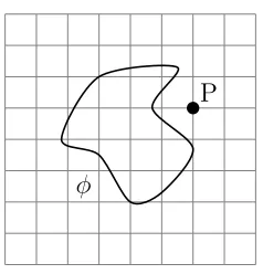
As mentioned in the introduction, distance field can be signed or unsigned. A signed distance field is a representation of the shortest distance from any point on the grid to the interface of an object represented as a polygonal model. The interface describes the isocontour of a shape in two or more dimensions and is defined by a signed distance functionφ. Figure 2.1 shows an interface represented byφ in a two-dimensional (_R2₎ grid. For a pointP ∈_R2_{, the signed distance from} _P _{to the interface is positive if} _P is outside its boundary, negative if P is inside its boundary and zero if P lies on the interface itself. In Figure 2.1, point P has a positive distance value since it is located outside of the interface boundary. Figure 2.2 exhibits a slice of the signed distance field of complex three dimensional geometries.

φ

P

(26)

2.1.1 Calculating Signed Distance Field

There are two general approaches for calculating the signed distance field. The first is geometric that includes brute-force, distance meshing [11], scan conversion [8], prism scan [32] etc. For example, in a brute-force approach, M line segments are drawn from a point on the grid to the boundary of the closest object. Then the minimum distance to allM line segments is calculated for each point of interest. The algorithmic complexity of the brute-force approach isO(N∗M) where N is the total number of grid points and M is the number of line segments. The implementation of such methods are complex and can be very slow compared to numerical methods.

Figure 2.2: Distance field visualization of the Stanford Dragon (left) and the Stanford Bunny (right)

The second approach applies numerical methods to calculate the distance field. Fortunately mathematicians were able to generalize the distance field problem to a non-linear partial differential equation governed by the eikonal equation. Since, the brute force approach is computationally expensive and therefore, impractical to use in most applications, this research focuses on solving the eikonal equation.

2.1.2 The Eikonal Equation

(27)

microscope. These secondary electrons are used to modulate appropriate devices to create a shape of the object by solving the eikonal equation [5].

Definition The eikonal equation is a first order, non-linear, hyperbolic partial dif-ferential equation of the form

|∇φ(x)|=f(x), for x∈Ω⊂_Rn, φ(x) = g(x), for x∈Γ⊂Ω

(2.1)

where, φ is the unknown, f is a given inverse velocity field, g is the value of φ at an interface Γ, Ω is an open set in _Rn_, _∇ _{denotes the gradient and} _|.| _{is the euclidean}

norm.

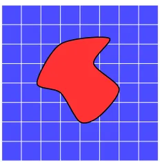
The eikonal equation is also fundamental to solving the interface propagation problem. To explain that problem consider Figure 2.3, which depicts an interface that is represented by the black curve that separates a red inside region from a blue outside region. Each point on the interface either moves towards the outside region or the inside region with either the same or different known speed values. The direction of propagation of the interface at each point, either inward or outward, is indicated by the sign of the speed values: negative for inside and positive for outside.

Figure 2.3: 2D shape with inside and outside regions separated by an interface

(28)

and the blue region can represent water. Then, the propagation of the boundary enclosing the red region can be determined either by the melting of ice, that shrinks the red region or the freezing of ice, that expands the red region. The goal is to track the interface as it evolves. Since, interfaces can be expanding and contracting at different points, f(x) can be negative at some points and positive at others. The general solution of the eikonal equation is the shortest amount of time (or arrival time) the interface will take to propagate to that point given some known f(x). The degenerate case when f(x) = 1 means all points propagate with the same speed (i.e., one grid cell per time interval). As a result, the solution of the eikonal equation for f(x) can be interpreted as the shortest distance from the interface to that point. Hence the special case of the solution to the eikonal equation wheref(x) = 1 is known as the signed distance function.

Definition The signed distance function for any given closed set S of points, is

dS(p) = min

x∈S ||p−x||

that is,dSis the distance to the closest point in S. If S divides space into a well-defined

regions, then the signed distance function is

φS = 

 

 

−dS(p) :p is inside,

dS(p) :p is outside 

 

 

Following the derivation in [4], the eikonal equation for calculating the signed distance is written as follows:

|∇φ|= 1 (2.2)

(29)

2.2 Solution Algorithms

Some of the well known methods for solving the interface propagation problem are Dijkstra’s algorithm [33], Fast Marching Method [30] and Fast Sweeping Method [40]. These methods improve upon the previous work and provide a different perspective on the problem. The following subsections explore these methods in more detail. 2.2.1 Dijkstra’s Algorithm

Dijkstra’s single source shortest path algorithm [33], based on discrete structures, can also be adapted to solve this problem [9]. It is a graph search algorithm, developed by Edsger Dijkstra in 1959, that finds the shortest path from one node to another. It is ubiquitous; everywhere from network routing to a car’s navigation system [30]. In the context of distance field, this is in essence what we want to find; the shortest distance from a source point to an object. This method is a very intuitive way to solve this problem with the following basic steps:

1. Start with a source node and initialize the cost to be 0. 2. Initialize tentative cost at all other nodes to ∞.

3. Mark the start node as accepted and keep track of the list of accepted nodes. 4. Calculate the cost of reaching the neighbor nodes which are one node away. 5. Update the cost if it is less than previous.

6. Mark the node with the least cost as accepted. 7. Repeat until all nodes are accepted.

(30)

1996 created a numerical method called fast marching method [30], similar to the Dijkstra’s algorithm for solving the continuous eikonal problem.

Start

End

1/2 1/3 1/4 1/3 1/1 1/2 1/1 1/3 1/4 1/5 1/2 1/3 1/3 1/4 1/2 1/3 1/2 1/4 1/2 1/2 1/3 1/4 1/2 1/3

Figure 2.4: Dijkstra’s algorithm finding the shortest path (shown in red). Actual shortest distance is the diagonal (shown in blue).

2.2.2 Fast Marching Method (FMM)

FMM is one of the popular techniques for solving the eikonal equation. It is also a one-pass algorithm similar to Dijkstra’s but uses upwind difference operators to approximate the gradient [31]. The grid points are updated in order of increasing distance with the aid of a difference formula. Starting with the initial position of the interface, FMM systematically marches outwards one grid point at a time, relying on entropy-satisfying schemes to produce the correct solution [31]. It needs a sorting algorithm that isO(log(N)) whereN is the number of grid points. Therefore, the FMM has an algorithmic complexity of order O(N log(N)). The advantage of FMM is that it allows for calculation of narrow bands of data near the surface. The disadvantages of this method are that it is difficult to implement, has an additional log(N) factor added by the sorting algorithm and is challenging to parallelize. 2.2.3 Fast Sweeping Method (FSM)

(31)

It uses nonlinear upwind difference scheme and alternating sweeping orderings of Gauss-Seidel iterations on the whole grid until convergence [40]. The advantage of FSM is that it is straightforward and has linear runtime complexityO(N) forN grid points.

Consider a three-dimensional domain discretized into a grid with NI, NJ, NK nodes in the x-, y-, and z- directions, respectively. Let Γ be a two dimensional interface describing the initial location from which the solution propagates. Then the Godunov upwind differencing scheme on the interior nodes used by the FSM as represented in [29] is:

φi,j,k −φxmin

dx

2

+

φi,j,k−φymin

dy

2

+

φi,j,k −φzmin

dz

2

=f_i,j,k2 (2.3)

for i∈ {2, . . . , N I−1},j ∈ {2, . . . , N J−1}, andk ∈ {2, . . . , N K−1}where,φxmin =

min(φi−1,j,k, φi+1,j,k),φymin=min(φi,j−1,k, φi,j+1,k), andφzmin=min(φi,j,k−1, φi,j,k+1). In this thesis, the implementations of FSM will only be solved for computing the signed distance field i.e., Equation (2.2). Therefore, the right hand side of Equation (2.3) is set to 1 (i.e., f = 1). Equation (2.3) then becomes

φi,j,k −φxmin

dx

2

+

φi,j,k−φymin

dy

2

+

φi,j,k−φzmin

dz

2

= 1 (2.4)

Gauss-Seidel iterations with alternating sweeping orderings are performed to solve Equation (2.1), until the solution converges for every point. The convergence for all points is guaranteed by the characteristic groups formed by an interface containing initial values. According to Zhao [40], there is a finite amount of interface character-istic groups, so a finite amount of sweeps is required for point solution to converge. The number of iterations to ensure convergence depends on the number of dimensions in a grid. Approximately 2n ∈ _Rn ₍₂2 _∈

(32)

dimensions. The fast sweeping algorithm consists of two main phases: initialization and sweeping.

1. Initialization: The grid is initialized by first setting the known interface bound-ary values in the grid. As soon as the interface points are initialized, all the other points in the grid are set to large positive values. During the sweeping phase of the algorithm, interface points do not change, while the rest of the points get updated to new smaller values using characteristic groups of the interface points.

2. Sweeping: The sweeping phase of the algorithm performs several Gauss-Seidel iterations. These iterations do not change interface boundary points that are fixed during the initialization phase. Sweeping iterations update the distance values for points that were not fixed at initialization phase. New distance value for a point is solved by selecting the minimum value between the current and the calculated value. This assures that the solution for a point will remain non-increasing. Alternating sweeping ordering is used to ensure that the information is being propagated along all (4∈_R2 _{and 8}_∈

R3) classes of characteristics. In [40], Zhao showed that this method converges in 2n sweeps in _Rn and that the convergence is independent of the size of the grid.

The nodes with the red dots in Figure 2.5, indicate an updated solution during the calculation of the first sweep ordering in two dimensions. The possible sweep directions to guarantee convergence in three dimensions are listed below:

(a) i = 1:NI, j = 1:NJ, k = 1:NK (b) i = NI:1, j = 1:NJ, k = NK:1 (c) i = 1:NI, j = 1:NJ, k = NK:1 (d) i = NI:1, j = 1:NJ, k = 1:NK

(e) i = NI:1, j = NJ:1, k = NK:1 (f) i = NI:1, j = NJ:1, k = 1:NK (g) i = NI:1, j = NJ:1, k = 1:NK (h) i = 1:NI, j = NJ:1, k = NK:1

(33)

Algorithm 1: Fast Sweeping Method [40] in 3D

1 initialize(φ);

2 for iteration= 1 to max iterationsdo 3 for ordering = 1 to 23 do

4 change axes(ordering); 5 for i= 1 to N I do 6 for j = 1 to N J do

7 for k = 1 to N K do

8 update(φ_i,j,k);

9 end

10 end

11 end

12 end

13 end

line 2 increases the accuracy of the solution. The for-loop in line 3 represents the sweeping phase, where line 4 rotates the axis to perform sweeping in a different direction and line 8 solves Equation (2.4). Although there are several methods for solving the eikonal equation, this thesis focuses on the FSM by Zhao [40] because of its straightforward implementation and linear time algorithmic complexity. However, the performance gained from Algorithm 1, may not be sufficient for practical use in application domains like real-time rendering and motion planning or solve large problems that require large memory. Therefore, researchers are always investigating faster methods and designing parallel algorithms to improve performance of existing methods. The following sections discusses the parallel algorithms that improves the performance of FSM.

2.3 Parallel Algorithms for FSM

(34)

I J

1 2 1 2

Figure 2.5: The first sweep ordering of FSM for a hypothetical distance function calculation from a source point (center) [7]

nodes, makes it challenging to design an efficient parallel algorithm without causing a decay in the convergence rate. Nonetheless, research efforts produced algorithms for parallelizing FSM.

2.3.1 Parallel Algorithm of Zhao

Zhao presented a parallel implementation of FSM [41] by leveraging the causality of the partial differential equation, i.e., when a grid value reaches the smallest possible value it is the solution and will not be changed in later iterations. This simple causality allowed implementation of different sweeping ordering in parallel, i.e., each sweep is assigned to different threads (or processes) and is computed simultaneously. Each of the threads generate a separate temporary solution which is reduced to a single solution by taking the minimum value from all the temporary solutions. For example, in _R2 _{there are four sweepings which are assigned to four different threads.} After each thread is done with its sweeping the four solutions φ1, φ2, φ3, and φ4 are synchronized using

φ =min(φ1, φ2, φ3, φ4)

(35)

parallel sweep

(φ1) (φ2) (φ3) (φ4)

min(φ1, φ2, φ3, φ4)

(φ)

Figure 2.6: Parallel FSM of Zhao in 2D

This method sets a lower upper bound on the degree of parallelization that can be exploited. For example, it instantiates up to four threads in two spatial dimensions and eight threads in three spatial dimensions. The algorithm can be implemented using either OpenMP in a shared memory environment or MPI in a cluster environment. In order to increase the parallelization, Zhao also proposed a domain decomposition approach for parallelizing FSM that could potentially utilize any arbitrary number of threads [41]. However, the performance of the domain decomposition approach plateaus with the increase in the number of threads. This is due to the communication overhead of passing the boundary values back and forth among the threads. Hence, this approach is not discussed in this thesis.

(36)

(in 2D) and 8 (in 3D) times more memory resources, 3) it creates synchronization overhead and is not suitable for massively parallel architectures such as GPUs. A pseudo-code of Zhao’s parallel algorithm is shown in Algorithm 2.

Algorithm 2: Parallel Fast Sweeping Method of Zhao [41] in 3D

1 initialize(φ);

2 for iteration= 1 to max iterationsdo 3 parallel for ordering = 1 to 23 do

/* change the direction of the sweep ordering based on the

thread number */

4 change axes(ordering); 5 for i= 1 to N I do 6 for j = 1 to N J do

7 for k = 1 to N K do

8 update(φ_i,j,k);

9 end

10 end

11 end

12 end

13 φ =min(φ1, . . . , φ8); 14 end

In Algorithm 2 the block of code in lines 4−11 is executed in parallel by each of the 23 threads. After the distance values are calculated by each thread the solution at each point in the grid is reduced by taking the minimum value calculated for that point which is represented by line 13 in Algorithm 2.

2.3.2 Parallel Algorithm of Detrixhe et al.

(37)

Detrixhe et al. [7] classify each node on the grid to a level based on the sum of the node’s coordinates. In 2D, the level of a node (i, j) is defined aslevel =i+j as shown in Figure 2.7(a) and in 3D, the level of a node (i, j, k) is defined aslevel=i+j+kas shown in 2.7(b). In_Rn_{, this ordering allows for a (2}_n_{+ 1)-point stencil to be updated}

independently of any other points within a single level.

I J

1 2 1 2 Level= 2 Level= 3 Level=I+ 1

(a)

(1,1,1) (1,1,1) Level= 3 Level= 4

I J

K

(b)

Figure 2.7: Cuthill-McKee ordering of nodes into different levels [7] in two dimensions (left) and three dimensions (right)

Although this approach is not straightforward as Zhao’s parallel algorithm [41], it offers significant advantages such as

• The same, as in the serial implementation, number of iterations required for the computation to converge.

• No extra memory resources are required comparing to Algorithm 2. • No synchronization overhead.

• The level of parallelism is not limited by the number of threads.

(38)

the increase in number of threads, it is well suited for massively parallel architectures (such as GPUs). These architectures have high number of hardware cores and less overhead of spawning threads than on a CPU architecture.

Algorithm 3: Parallel Fast Sweeping Method from Detrixhe et al. [7]

1 initialize(φ);

2 for iteration= 1 to max iterationsdo 3 for ordering = 1 to 23 do

4 change axes(ordering);

5 for level= 3 to N I+N J+N K do 6 N I₁ =max(1, level−(N J+N K)); 7 N I2 =min(N I, level−2);

8 N J₁ =max(1, level−(N I+N K)); 9 N J2 =min(N J, level−2);

10 parallel

/* Each combination of (i, j) generated from the for loops below is executed in parallel */

11 for i=N I1 to N I2 do 12 for j =N J₁ to N J₂ do 13 k =level−(i+j);

14 if k > 0 and k <=N K then

15 update(φ_i,j,k);

16 end

17 end

18 end

19 end

20 end

21 end

2.3.3 Hybrid Parallel Algorithm

(39)

Algorithm 4: Hybrid Parallel Fast Sweeping Method using Algorithm 2 and 3

1 initialize(φ);

2 for iteration= 1 to max iterationsdo 3 parallel for ordering = 1 to 23 do

/* change the direction of the sweep ordering based on the

thread number */

4 change axes(ordering);

5 for level= 3 to N I+N J+N K do 6 N I₁ =max(1, level−(N J+N K)); 7 N I2 =min(N I, level−2);

8 N J₁ =max(1, level−(N I+N K)); 9 N J2 =min(N J, level−2);

10 parallel

/* Each combination of (i, j) generated from the for loops below is executed in parallel */

11 for i=N I₁ to N I₂ do 12 for j =N J1 to N J2 do 13 k =level−(i+j);

14 if k > 0 and k <=N K then

15 update(φi,j,k);

16 end

17 end

18 end

19 end

20 end

21 φ =min(φ1, . . . , φ8); 22 end

Although it might be intuitive to think that this algorithm will perform better than Algorithms 2 and 3 since, the algorithm employs multi-level parallelism (coarse-grain and fine-grain). However, it still retains the same disadvantages that were discussed in Section 2.3.1 that could impact the performance. There is also the added performance overhead associated with communication and reduction of the final solution from the results of different processes. Therefore, it is important to compare the performances between the various implementation of these algorithms. Chapter 4 will present and analyze this data.

(40)

algorithms, the FSM solver can be implemented in various specialized hardware accel-erators and architecture models. The following section discusses parallel architectures and different types of hardware accelerators available today.

2.4 Hardware Accelerators

Accelerators refer to specialized computer hardwares that have higher potential to increase performance of certain computational functions compared to a general pur-pose processor. Accelerators such as GPUs and Intel co-processors are specialized for performing floating point operations. These hardware accelerators allow greater parallelization of tasks due to their high number of cores with the added advantage of reduced overhead of instruction control to improve the execution of certain programs. The Flynn’s taxonomy, a classification system proposed by Michael J. Flynn, classifies these architectures as Single Instruction, Multiple Data (SIMD) architecture. This classification system is based upon the number of concurrent instruction streams and data streams available in the architecture and is used as a reference in designing modern processors. There are four classifications in Flynn’s taxonomy and they are as follows:

• Single Instruction, Single Data (SISD): This architecture model is found in sequential computer where a single operation is performed at a time, using a single data stream. The traditional uniprocessor machines and older personal computers are examples of SISD architecture.

• Single Instruction, Multiple Data (SIMD): This architecture model is found in modern processors that have multiple cores where a single instruction is carried out by multiple cores but on different data streams. SIMD architectures exploit data parallelism to increase performance of certain programs. GPUs and multi-core processors are examples of SIMD architecture.

(41)

• Multiple Instruction, Multiple Data (MIMD): This architecture model is found in systems with number of autonomous processors that can concurrently execute different instructions on different data. Distributed systems is an example of MIMD architecture.

Although modern CPUs are multi-core and often feature parallel SIMD units; the use of accelerators still yields benefits. The two types of hardware accelerators is discussed in more detail in the following subsections.

2.4.1 Graphics Processing Unit (GPU)

GPU is a single-chip processor especially designed for performing calculations related to 3D computer graphics such as lighting effects, object transformations and 3D motion. These are embarrassingly parallel calculations, that exhibit massive data parallelism, for which GPUs are designed to perform extremely well. The multi-billion dollar gaming industry exerts tremendous economic pressure for the ability to perform massive number of floating point calculations per video frame in advance games and hence, drives the development of the GPUs [15]. As a result, GPUs are designed as a throughput oriented device i.e., it is optimized for the execution throughput of massive number of threads. GPUs require large number of executing threads to hide the long-latency memory accesses. Thus, minimizing the control logic required for each execution thread. [15] “GPUs have small cache size to help control the bandwidth requirements of these applications so multiple threads that access the same memory data do not need to all go to the DRAM. Hence, more chip area is dedicated to the floating-point calculations” [15].

(42)

using GPU (known as GPGPU), has positioned the GPU as a compelling alternative to traditional microprocessors in high-performance computer systems of the future [23].

Figure 2.8: CPU and GPU fundamental architecture design. [19]

Figure 2.8 depicts the general design diagrams of CPUs and GPUs. CPUs have few cores with high clock frequencies along with larger areas allocated to cache and a control unit. Such design allows CPUs to perform a single task efficiently. Whereas, GPUs have hundreds of cores with low clock frequencies, small cache area and simple control units. Thus, GPUs are designed to perform several multiple similar tasks simultaneously. Therefore, GPUs do not perform well on tasks where different instructions are carried out sequentially. As a consequence, CPU and GPU are used alongside of each other where the sequential code are executed on the CPU and numerically intensive parallel code on the GPU.

(43)

Figure 2.9: A schematic of the CPU/GPU execution [21].

2.4.2 Intel Xeon Phi Co-processor

Intel’s Xeon Phi co-processor, exemplifies the many integrated core (MIC) architec-ture and is another example of a hardware accelerator. It contains up to 61 small, low-power processor cores on a single chip to provide a high degree of parallelism and better power efficiency [28]. One advantage Intel’s co-processors have over GPUs is that it can operate independently of CPUs and they don’t require specialized pro-gramming [6]. Another advantage is that the co-processor has “x86-compatible cores with wide vector processing units and uses standard parallel programming models, such as MPI, OpenMP, and hybrid MPI+OpenMP, which makes code development simpler” [28]. Each of the cores support four hardware threads, i.e. each core can concurrently execute instructions from four threads or processes. This keeps the execution units busy by reducing the vector pipeline and memory access latencies [25]. The on chip memory on an Intel Xeon Phi is not shared with the host processor. Thus, copying of data to and from the host and co-processor memories is necessary. This communication between the co-processor and the host processor goes through the PCI Express bus [28] that causes the added latency to data transfers.

(44)

kernel and supports MPI and OpenMP. There are three common execution models for programming and execution of applications for Xeon Phi coprocessors and can be categorized as follows [26]:

• Offload execution mode: In this mode the application starts execution on the host node and the instructions of code segments annotated with offload directives are sent to the coprocessor for execution. This is also known as heterogeneous programming mode.

• Coprocessor native execution mode: Since, Intel Xeon Phi runs a micro Linux operating system the users can view it as a compute node and can execute code directly on the coprocessor.

• Symmetric execution mode: In this mode the application executes on both the host and the coprocessor. Communication between the host and the coprocessor is usually done through message passing interface.

Due to the increasing popularity of accelerators and co-processors, various pro-gramming models have been developed by different communities to make program-ming easier for these devices. Although NVIDIA GPU hardware is used as the chosen accelerator, but the algorithms themselves are general and not specific to GPUs. The following section discusses some of the available frameworks and models for programming accelerators.

2.5 Programming Models

(45)

NVIDIA to add features to facilitate the ease of parallel programming using GPUs [15].

As a result, NVIDIA made changes to its hardware and released CUDA (Compute Unified Device Architecture) in 2007 [15] that made GPGPU implementation easier and faster to learn. Currently there are other platforms like OpenCL, OpenMP and OpenACC that provide different constructs for running code on various accelerators including GPU and Intel Xeon Phi coprocessor. However, none of the above plat-forms address multi-GPU parallelism across different nodes therefore, multiple GPU implementation must be explicitly performed by the developer [37]. Libraries such as MPI or POSIX can be associated with CUDA and OpenACC in order to benefit from a GPU cluster. The programming models used and discussed in this research are CUDA, OpenACC and MPI.

2.5.1 Compute Unified Device Architecture (CUDA)

CUDA is a parallel computing platform and a library interface developed by NVIDIA to harness massively parallel computing architecture of modern NVIDIA GPUs. The CUDA interface is a proprietary of NVIDIA and can only be used with NVIDIA GPUs. “The CUDA architecture is built around a scalable array of multithreaded streaming multiprocessors (SMs)” [19] each containing a group of execution cores. For example, Tesla K40 has 2880 cores distributed over 15 SMs, each of those SMs have 192 cores [28]. Before using CUDA for GPU programming, it is important to understand some basic CUDA concepts [27]. CUDA-enabled GPUs run in a memory space separate from the host processor. Hence, data must be transferred from the host to the device for performing calculations by using one of the data transfer mechanisms provided by CUDA. Explicit data transfers can be done using API such as

(46)

a value”[27]. Kernel calls are asynchronous thus, the programmer need to explicitly call synchronization API such as cudaThreadSynchronize() to act as a barrier.

A thread is the basic unit of work on the GPU [27]. As illustrated in Figure 2.10, CUDA follows a thread hierarchy arranged in a 1D, 2D or 3D computational grid composed of 1D, 2D or 3D thread blocks. An executional configuration of a CUDA kernel encloses the configuration information, that defines the arrangement of threads, between triple angle brackets <<< >>>. “When a kernel is invoked by the host CPU of a CUDA program, the blocks of the grid are enumerated and distributed to multiprocessors with available execution capacity” [19]. The threads of a thread block execute concurrently on one multiprocessor in a SIMD manner, i.e., all threads execute the same instruction but with different data streams. Furthermore, multiple thread blocks can execute concurrently on one multiprocessor. As thread blocks finish execution, new blocks are launched on the available multiprocessors [19]. In addition to thread blocks, CUDA defines a wrap, which is a collection of 32 threads. At any time an SM can execute a single warp.

(47)

Figure 2.10 depicts the memory hierarchy of CUDA which is similar to a conven-tional multiprocessor. The fastest and the closest to the core are the local registers. The next closest and fastest memory is the shared memory. All the threads from a single grid block can access shared memory and can synchronize together. Threads from different grid blocks cannot synchronize. Thus, the exchange of data is only possible through the global memory. The shared memory is similar to the L1 cache on a CPU, as it provides very fast access and stores data that is accessed frequently by multiple threads [37]. The only downside is that the shared memory must be maintained by the programmer explicitly. The next memory in this hierarchy is the global memory, i.e., the memory space that can be addressed by any thread from any grid block but has a high latency cost. Therefore, coalesced memory access is crucial when accessing global memory as it can hide the latency cost. Global memory accesses can be coalesced in a single transaction if thread blocks are created as a multiple of 16 threads i.e., half warp [28]. Note, that for each GPU architecture there is a maximum number of threads per block that can be run per multiprocessor. Therefore along with the parallelization of the code, optimization of the memory accesses using shared memory and the coalesced access to global memory is also a significant challenge in the development process.

The next available type of memory is called constant memory, which is stored on chip. It is used for allocating fixed data, i.e. data that won’t change during the execution of a kernel. And the final type of memory in CUDA is the texture memory. The texture memory is also stored on chip and optimized for 2D spatial locality. When coalesced read cannot be achieved, it is preferred to use texture memory than global memory [37]. To illustrate a CUDA kernel using CUDA-C, consider the code in Listing 2.1 where the host code invokes a a CUDA kernel that adds two vectors.

/* CUDA kernel */

__global__ void add_vector(int n, float *x, float *y)

(48)

/* Calculate unique 1D index from 2D thread block */ int i = blockIdx.x * blockDim.x + threadIdx.x;

if (i < n) y[i] = x[i] + y[i];

}

int main(void)

{

. . .

/* Allocate memory on GPU */

cudaMalloc(&d_x, n * sizeof(float));

cudaMalloc(&d_y, n * sizeof(float));

/* Copy data from host to GPU */

cudaMemcpy(d_x, x, n * sizeof(float), cudaMemcpyHostToDevice);

cudaMemcpy(d_y, y, n * sizeof(float), cudaMemcpyHostToDevice);

/* Execute the code on the GPU using 2D grid block */ add_vector<<<(n+255)/256, 256>>>(n, d_x, d_y);

/* Copy data from GPU to host */

cudaMemcpy(y, d_y, n * sizeof(float), cudaMemcpyDeviceToHost);

. . .

}

Listing 2.1: An example of a CUDA kernel using the C programming language that adds two vectors. The text in red represents the API and reserved keywords in CUDA.

2.5.2 Open Accelerators (OpenACC)

(49)

2.1 lists the supported platforms by various commercial OpenACC compilers (PGI, PathScale and Cray).

OpenACC directives provide an easy and powerful way of leveraging the advan-tages of accelerator computing while keeping the code compatible with CPU only systems [20]. A typical scenario of a computing system would be the CPU as the host and the GPU as the accelerator. If an accelerator is not present then the compiler ignores the directives and generates machine code that runs on the CPU. The host and the accelerator have separate memory spaces, therefore, OpenACC provides directives that handles the transfer of the data between the host and the accelerator. Thus, abstracting the details of the underlying implementation and significantly simplifying the tasks of parallel programming and code maintenance. The common syntax for writing an OpenACC pragma in C/C++ is

#pragma acc directive-name [clause [[,] clause]...] newline

Table 2.1: Platforms supported by OpenACC compilers [22].

Accelerator PGI PathScale Cray x86 (NVIDIA Tesla) Yes Yes Yes x86 (AMD Tahiti) Yes Yes No

x86 (AMD Hawaii) No Yes No

x86 multi-core Yes Yes No

ARM multi-core No Yes No

(50)

void add_vector(int n, float *x, float *y)

{

#pragma acc kernels

for(int i = 0; i < n; ++i) {

y[i] = x[i] + y[i];

} }

Listing 2.2: An example of a loop parallelized using OpenACC. The text in red represents the OpenACC keywords.

Here the #pragma acc line indicates that it is an OpenACC compiler directive and simply suggests the compiler to attempt to generate parallel code for the targeted accelerator. Comparing the two code fragments in Listings 2.1 and 2.2, it is clear that OpenACC requires fewer code modifications, is simple to program and easier to understand than CUDA. For reasons of portability, simplicity and code maintenance using OpenACC for acceleration is advantageous than using CUDA.

2.5.3 Message Passing Interface (MPI)

MPI is a standard specification for message passing libraries based on the consensus of the MPI Forum, that consists of vendors, developers and users. The goal of MPI is to provide a portable, efficient and flexible interface standard for writing message passing programs. In message passing programming model, data located on the address space of one process is moved to the address space of another process through cooperative operations [2]. Thus, enabling developers to communicate between different processes to create parallel programs. MPI was originally designed for networks of workstations with distributed memory. However, as architecture changed to shared memory sys-tems, MPI adapted to handle a combination of both types of underlying memory architectures seamlessly [2]. As a result, MPI is widely used and considered as an industry standard for writing message passing applications.

(51)

to execute in MIMD manner through streams. The discussion of CUDA streams is beyond the scope of this thesis. Each process in MPI is identified with consecutive integers starting at 0, according to their relative rank in a group. “The processes communicate via calls to MPI communication primitives. Typically, each process executes in its own address space, although shared-memory implementations are also possible” [34]. The basic communication mechanism is the point-to-point communi-cation, where data is transmitted between a sender and a receiver. Then, there is collective communication where data is transmitted to group of processes specified by the user. MPI also supports both blocking and non-blocking communications between processes. Non-blocking communication allows developers to increase performance by overlapping communication and execution between processes. Along with predefined data types, MPI also permits user-defined data types for heterogeneous communica-tion. A simple example of a C code using MPI, where process 0 sends a message to process 1, is presented below:

int main(int argc, char *argv[])

{

char msg[15]; int myRank; int tag = 0;

MPI_Init(&argc, &argv);

MPI_Request req;

MPI_Status status;

/* find process rank */

MPI_Comm_rank(MPI_COMM_WORLD, &myRank);

MPI

if (myRank == 0) {

strcpy(msg, "Hello World!");

MPI_Isend(msg, strlen(msg)+1, MPI_CHAR, 1, tag,

MPI_COMM_WORLD, &req);

MPI_Wait(&req, &status);

} else if (myRank == 1) {

(52)

MPI_Wait(&req, &status);

}

MPI_Finalize();

return 0;

}

Listing 2.3: An example of MPI communication. The text in red represents the MPI keywords and API.

2.6 Parallel FSM Implementations

2.6.1 Common Implementation Details

Most of the code for the distance field solver is identical across all parallel implemen-tations and are not considered as part of the FSM algorithm. There are number of steps carried out before and after the execution of the FSM algorithm, including

1. Open and parse the input file that contains the information about the geometry. The file is saved with a .vti/.nc extension.

2. Boundary values are added to each dimension of the domain and set to some default values.

3. The FSM algorithm is executed.

4. The distance values of the points that lie inside of an object are set to -1. 5. The default boundary values set in the second step are adjusted by copying the

values of the nearest neighbor.

(53)

2.6.2 MPI Implementation of Zhao’s Method

The parallel sweeping algorithm for FSM described in Section 2.3.1 Algorithm 2 is implemented here using MPI, with pseudocode shown in Listing 2.4.

int index, totalNodes;

// specifies the sweeping directions int sweeps[8][3] = { { 1, 1, 1 },

{ 0, 1, 0 },

{ 0, 1, 1 },

{ 1, 1, 0 },

{ 0, 0, 0 },

{ 1, 0, 1 },

{ 1, 0, 0 },

{ 0, 0, 1 } };

// temporary array to store the reduced solution double * tmp_distance;

if(my_rank == MASTER) {

// if there are more than 1 PEs then the // temporary array is required to store the // final distance values after min reduction

if (npes > 1) {

tmp_distance = (double *) malloc( totalNodes * sizeof(double) );

} }

for (int s = my_rank; s < 8; s += npes) {

int iStart = (sweeps[s][0]) ? 1 : pf->z; int iEnd = (sweeps[s][0]) ? pf->z + 1 : 0;

int jStart = (sweeps[s][1]) ? 1 : pf->y; int jEnd = (sweeps[s][1]) ? pf->y + 1 : 0;

int kStart = (sweeps[s][2]) ? 1 : pf->x; int kEnd = (sweeps[s][2]) ? pf->x + 1 : 0;

for (int i = iStart; i != iEnd; i = (sweeps[s][0]) ? i + 1 : i - 1) { for (int j = jStart; j != jEnd; j = (sweeps[s][1]) ? j + 1 : j - 1) {

for (int k = kStart; k != kEnd; k = (sweeps[s][2]) ? k + 1 : k - 1) {

index = i * max_xy + j * max_x + k;

pf->distance[index] = solveEikonal(pf, index);

(54)

}

MPI_Barrier(MPI_COMM_WORLD);

// reduce the solution if there are more than 1 PE if( npes > 1 ) {

MPI_Reduce(pf->distance, tmp_distance, totalNodes, MPI_DOUBLE, MPI_MIN, MASTER, MPI_COMM_WORLD);

if( my_rank == MASTER ) { free( pf->distance );

pf->distance = tmp_distance;

} }

Listing 2.4: Code fragment that implements the sweeping stage of the parallel FSM algorithm by Zhao [41], Algorithm 2, using MPI.

2.6.3 CUDA Implementation of Detrixhe et al.’s Method

The parallel algorithm for FSM described in Section 2.3.2 Algorithm 3 is implemented here using CUDA, with pseudocode shown in Listing 2.5. The CUDA kernel in this implementation is executed for each level of the Cuthill McKee ordering for all sweeping directions. Since, each level has different number of mesh points, the kernel is executed with different configuration of two dimensional thread block and grid arrangements. However, when the number of mesh points is equal to or greater than 256, the kernel is executed with (16×16) thread block and two dimension grid size that encompasses the total number of mesh points.

for (int swCount = 1; swCount <= 8; ++swCount) {

int start = (swCount == 2 || swCount == 5 ||

swCount == 7 || swCount == 8) ? totalLevels : meshDim; int end = (start == meshDim) ? totalLevels + 1 : meshDim - 1;

int incr = (start == meshDim) ? true : false;

// sweep offset is used for translating the 3D coordinates // to perform sweeps from different directions

(55)

for (int level = start; level != end;

level = (incr) ? level + 1 : level - 1) { int xs = max(1, level - (sw.yDim + sw.zDim)); int ys = max(1, level - (sw.xDim + sw.zDim)); int xe = min(sw.xDim, level - (meshDim - 1)); int ye = min(sw.yDim, level - (meshDim - 1));

int xr = xe - xs + 1, yr = ye - ys + 1;

int tth = xr * yr; // Total number of threads needed

dim3 bs(16, 16, 1); if (tth < 256) {

bs.x = xr; bs.y = yr;

}

dim3 gs(iDivUp(xr, bs.x), iDivUp(yr, bs.y), 1);

sw.level = level; sw.xOffSet = xs; sw.yOffset = ys;

fast_sweep_kernel <<<gs, bs>>> (dPitchPtr, sw); cudaThreadSynchronize();

} }

Listing 2.5: Host code fragment that implements the sweeping stage of the parallel FSM algorithm by Detrixhe et al. [7], Algorithm 3, and calls the CUDA kernel that executes parallel operations on the GPU.

__global__ void fast_sweep_kernel(cudaPitchedPtr dPitchPtr, SweepInfo s) {

int x = (blockIdx.x * blockDim.x + threadIdx.x) + s.xOffSet; int y = (blockIdx.y * blockDim.y + threadIdx.y) + s.yOffset;

if (x <= s.xDim && y <= s.yDim) { int z = s.level - (x + y); if (z > 0 && z <= s.zDim) {

int i = abs(z - s.zSweepOff); int j = abs(y - s.ySweepOff); int k = abs(x - s.xSweepOff);

char *devPtr = (char *)dPitchPtr.ptr; size_t pitch = dPitchPtr.pitch;

(56)

double *c_row = (double *)((devPtr + i * slicePitch) + j * pitch); double center = c_row[k];

double left = c_row[k-1]; double right = c_row[k+1];

double up = ((double *)

((devPtr + i * slicePitch) + (j-1) * pitch))[k]; double down = ((double *)

((devPtr + i * slicePitch) + (j+1) * pitch))[k]; double front = ((double *)

((devPtr + (i-1) * slicePitch) + j * pitch))[k]; double back = ((double *)

((devPtr + (i+1) * slicePitch) +j * pitch))[k];

double minX = min(left, right); double minY = min(up, down); double minZ = min(front, back);

c_row[k] = solve_eikonal(center, minX, minY, minZ, s.dx, s.dy, s.dz);

} } }

Listing 2.6: CUDA kernel that maps each thread to a grid point and calls the function that solves Equation (2.2) on that point.

(57)

the performance of the code by greater than 100× compared to the cudaMalloc

implementation.

cudaPitchedPtr hostPtr, devicePtr;

hostPtr = make_cudaPitchedPtr(pf->distance,

max_x * sizeof(double), max_x, max_y);

cudaExtent dExt = make_cudaExtent(max_x * sizeof(double), max_y, max_z);

// allocate memory on the device using cudaMalloc3D cudaMalloc3D(&devicePtr, dExt);

// copy the host memory to device memory cudaMemcpy3DParms mcp = 0 ;

mcp.kind = cudaMemcpyHostToDevice; mcp.extent = dExt;

mcp.srcPtr = hostPtr; mcp.dstPtr = devicePtr;

cudaMemcpy3D(&mcp);

Listing 2.7: CUDA-C code fragment that copies a three dimensional array from the host to the GPU.

2.6.4 OpenACC Implementation of Detrixhe et al.’s Method

The pseudocode for the parallel algorithm for FSM described in Section 2.3.2, Algo-rithm 3, implemented using OpenACC is shown in Listing 2.8.

int start, end, incr;

for (int sn = 1; sn <= 8; ++sn) {

SweepInfo s = make_sweepInfo(pf, sn);

start = (sn == 2 || sn == 5 || sn == 7 || sn == 8) ? s.lastLevel : s.firstLevel;

if (start == s.firstLevel) { end = s.lastLevel + 1; incr = 1;

} else {

end = s.firstLevel - 1; incr = 0;

(58)

level = (incr) ? level + 1 : level - 1) { // s - start, e - end

int xs, xe, ys, ye;

xs = max(1, level - (s.yDim + s.zDim)); ys = max(1, level - (s.xDim + s.zDim));

xe = min(s.xDim, level - (s.firstLevel - 1)); ye = min(s.yDim, level - (s.firstLevel - 1));

int i, j, k, index; int xSO = s.xSweepOff; int ySO = s.ySweepOff; int zSO = s.zSweepOff;

#pragma acc kernels {

#pragma acc loop independent for (int x = xs; x <= xe; x++) {

#pragma acc loop independent for (int y = ys; y <= ye; y++) {

int z = level - (x + y); if (z > 0 && z <= pf->z) {

i = abs(z - zSO); j = abs(y - ySO); k = abs(x - xSO);

index = i * max_xy + j * max_x + k;

pf->distance[index] = solveEikonal(pf, index);

} }

} // end of acc kernels

} } }

Listing 2.8: Code fragment that implements the sweeping stage of the parallel FSM algorithm by Detrixhe et al. [7], Algorithm 3, using OpenACC.

2.6.5 MPI/CUDA Implementation of Hybrid Parallel FSM

(59)

code block.

int my_rank, npes;

MPI_Comm_rank(MPI_COMM_WORLD, &my_rank); MPI_Comm_size(MPI_COMM_WORLD, &npes);

// temporary array to store the reduced solution double *tmp_distance;

int totalNodes = max_x * max_y * max_z;

if (my_rank == MASTER) {

// if there are more than 1 PEs then the temporary array

// is required to store the final distance values after min reduction if (npes > 1) {

tmp_distance = (double *) malloc(totalNodes * sizeof(double));

} }

cudaPitchedPtr hostPtr, devicePtr;

hostPtr = make_cudaPitchedPtr(pf->distance,

max_x * sizeof(double), max_x, max_y);

cudaExtent dExt = make_cudaExtent(max_x * sizeof(double), max_y, max_z);

cudaMalloc3D(&devicePtr, dExt);

_cudaMemcpy3D(hostPtr, devicePtr, dExt, cudaMemcpyHostToDevice);

// Each rank does a different sweep

for (int swCount = my_rank+1; swCount <= 8; swCount+=npes) {

int start = (swCount == 2 || swCount == 5 ||

swCount == 7 || swCount == 8) ? totalLevels : meshDim; int end = (start == meshDim) ? totalLevels + 1 : meshDim - 1;

int incr = (start == meshDim) ? true : false;

// sweep offset is used for translating the 3D coordinates // to perform sweeps from different directions

sw.xSweepOff = (swCount == 4 || swCount == 8) ? sw.xDim + 1 : 0; sw.ySweepOff = (swCount == 2 || swCount == 6) ? sw.yDim + 1 : 0; sw.zSweepOff = (swCount == 3 || swCount == 7) ? sw.zDim + 1 : 0;

(60)

int ye = min(sw.yDim, level - (meshDim - 1));

int xr = xe - xs + 1, yr = ye - ys + 1;

int tth = xr * yr; // Total number of threads needed

dim3 bs(16, 16, 1); if (tth < 256) {

bs.x = xr; bs.y = yr;

}

dim3 gs(iDivUp(xr, bs.x), iDivUp(yr, bs.y), 1);

sw.level = level; sw.xOffSet = xs; sw.yOffset = ys;

fast_sweep_kernel <<<gs, bs>>> (dPitchPtr, sw); cudaThreadSynchronize();

} }

_cudaMemcpy3D(devicePtr, hostPtr, dExt, cudaMemcpyDeviceToHost);