DEMOGRAPHIC RESEARCH
A peer-reviewed, open-access journal of population sciences
DEMOGRAPHIC RESEARCH
VOLUME 37, ARTICLE 17, PAGES 527–566
PUBLISHED 29 AUGUST 2017
http://www.demographic-research.org/Volumes/Vol37/17/ DOI: 10.4054/DemRes.2017.37.17
Research Article
Coherent forecasts of mortality with
composi-tional data analysis
Marie-Pier Bergeron-Boucher
Vladimir Canudas-Romo
Jim Oeppen
James W. Vaupel
c
2017 Marie-Pier Bergeron-Boucher et al.
1 Introduction 528
2 Methods 530
2.1 The Lee–Carter (LC) model 530
2.2 The Li–Lee model: LC-coherent 531
2.3 Forecasting with compositional data analysis (CoDa) 531
2.4 The CoDa-coherent model 533
3 Data 534
4 The underlying models 535
4.1 The parameters’ interpretation and forecasts 535
4.2 Explained variance and fitted models 537
5 Results 538
5.1 Evaluating the models 538
5.2 Life expectancy in 2050 541
5.2.1 More optimistic forecasts 541
5.2.2 Coherence in the forecasts 545
6 Discussion 546
7 Conclusion 547
8 Acknowledgement 547
References 549
Coherent forecasts of mortality with compositional data analysis
Marie-Pier Bergeron-Boucher1
Vladimir Canudas-Romo2
Jim Oeppen3 James W. Vaupel4
Abstract
BACKGROUND
Mortality trends for subpopulations, e.g., countries in a region or provinces in a country, tend to change similarly over time. However, when forecasting subpopulations indepen-dently, the forecast mortality trends often diverge. These divergent trends emerge from an inability of different forecast models to offer population-specific forecasts that are con-sistent with one another. Nondivergent forecasts between similar populations are often referred to as “coherent.”
METHODS
We propose a new forecasting method that addresses the coherence problem for subpop-ulations, based on Compositional Data Analysis (CoDa) of the life table distribution of deaths. We adapt existing coherent and noncoherent forecasting models to CoDa and compare their results.
RESULTS
We apply our coherent method to the female mortality of 15 Western European countries and show that our proposed strategy would have improved the forecast accuracy for many of the selected countries. The results also show that the CoDa adaptation of commonly used models allows the rates of mortality improvements (RMIs) to change over time.
CONTRIBUTION
This study opens a discussion about the use of age-specific mortality indicators other than death rates to forecast mortality. The results show that the use of life table deaths
1Max Planck Odense Center on the Biodemography of Aging, Institute of Public Health, University of
Southern Denmark, Odense, Denmark. E-Mail: [email protected].
2Max Planck Odense Center on the Biodemography of Aging, Institute of Public Health, University of
Southern Denmark, Odense, Denmark. E-Mail: [email protected].
3Max Planck Odense Center on the Biodemography of Aging, Institute of Public Health, University of
Southern Denmark, Odense, Denmark. E-Mail: [email protected].
and CoDa leads to less biased forecasts than more commonly used forecasting models based on the extrapolation of death rates. To the authors’ knowledge, the present study is the first attempt to forecast coherently the distribution of deaths of many populations.
1
Introduction
Accurate life expectancy forecasts are crucial inputs for decision-making by individuals and by financial, social, and health care institutions. The best way to obtain accurate fore-casts is still debated. Different methods for forecasting mortality have been introduced over the years. Booth and Tickle (2008) classify mortality forecasting models into three broad approaches: expert judgment, extrapolation of past trends, and epidemiological models. Most recent developments in forecasting mortality focus on extrapolative mod-els (Booth and Tickle 2008). The extrapolative approach generally finds its robustness in the linear changes over time of different indicators used for forecasts and the limited sub-jective judgment required (Stoeldraijer et al. 2013; Booth and Tickle 2008; Booth et al. 2006; Oeppen and Vaupel 2002).
A well-known extrapolative approach is the Lee–Carter model (Lee and Carter 1992). The Lee–Carter model uses linear extrapolations of the logarithms of age-specific death rates to forecast mortality, using principal component techniques. While the model works reasonably well (Lee and Miller 2001), one of its flaws is its assumption of a constant rate of age-specific mortality improvement over time. This assumption has been shown to be inadequate in many cases, especially at higher ages, and to overestimate the future level of mortality (Booth, Maindonald, and Smith 2002; Booth and Tickle 2008; Kannisto et al. 1994).
(Wilmoth 1995). It has been shown that when forecasts are based on cause-disaggregated measures, mortality forecasts by components tend to be dominated by an increase or slow decrease of certain subgroups, leading to more pessimistic forecasts (Wilmoth 1995). By using CoDa, this limitation can be avoided (Oeppen 2008).
An important issue related to extrapolative approaches to forecasting is that they of-ten do not consider analogous mortality trends for males and females or for countries in a region or provinces/states in a country. Mortality trends are often projected separately, which tends to increase the divergence between groups in the long run, even when using similar extrapolative procedures (Li and Lee 2005; Wilmoth 1995). Coherent forecasts, i.e., nondivergent forecasts, among industrialized countries are justified, since conver-gence of mortality levels across industrialized countries has been observed since the mid-dle of the 20th century (White 2002; Wilson 2001, 2011; Li and Lee 2005; Oeppen 2006). This occurred as a general process; populations became integrated via communication, transportation, trade, and technology, without however totally eliminating regional speci-ficities (Li and Lee 2005). Considering this convergence, forecasting mortality by single countries becomes less acceptable and coherent forecasts are often necessary (Li and Lee 2005; Schinzinger, Denuit, and Christiansen 2016; Bohk-Ewald and Rau 2017; Hynd-man, Booth, and Yasmeen 2013; Raftery et al. 2013; Cairns et al. 2011; Torri and Vaupel 2012).
Among the solutions offered for the regional coherence problem, Li and Lee (2005) suggest modifying the Lee–Carter method by identifying a factor for central tendency for a group of countries and a factor for individual-country trends. Carter and Lee (1992) and Russolillo, Giordano, and Haberman (2011) suggest using a single time-pattern of mortality change for many populations. Following a suggestion by Oeppen and Vaupel (2002), Torri and Vaupel (2012) forecast the best-practice in life expectancy, which has risen at a steady pace since 1840 (Oeppen and Vaupel 2002), and then forecast the gap between countries’ life expectancy and the record level. All these methods suggest using a common trend, reflecting a general mortality process, which influences the country-specific mortality.
Coherent regional mortality forecasts within a CoDa framework have not been ex-plored previously. In this article, we refer to CoDa methodology as a forecast performed within the CoDa framework. The main purpose of this study is to explore the use of an added common factor to the CoDa methodology to obtain an improved coherent forecast method based on the forecast of life table deaths.
compar-ing previous models with the new proposal. As final sections, a discussion and conclusion are included.
2
Methods
We compare four forecasting models: Lee–Carter and CoDa, both with and without a common factor. We briefly describe them here.
2.1 The Lee–Carter (LC) model
The Lee and Carter (1992) model is a principal components approach, based on the log-transformed age-specific death rates (mt,x). The model is written as:
ln(mt,x)−αx=κtβx+t,x, (1)
whereαxis the age-specific log-mortality average,κtis the level of mortality in yeart, βxis an age-pattern of mortality change at agex(also interpreted as the rate of mortality improvement once multiplied by the change inκtas shown in Appendix F), andt,xis the error term. The parametersκtandβxare the normalized first left and right singular vectors of the singular value decomposition (SVD) of the centered matrixlog(mt,x)−αx,
κt=uts 120 X
x=0
vx (2a)
βx=
vx 120 P
x=0 vx
, (2b)
2.2 The Li–Lee model: LC-coherent
Li and Lee (2005) modified the Lee–Carter model to forecast different populations in a coherent way. Their model uses a common factor, representing an average mortality trend for the whole group of countries. The death rates at timet, agexand for populationi, mt,x,i, are modeled as
log(mt,x,i)−αx,i−κtβx=kt,ibx,i+t,x,i, (3)
whereαx,i is the average log-mortality at a given agexfor populationi, andκtβx is the common factor for all populations. The common factor is obtained by applying the ordinary Lee–Carter method to the average mortality of the group, as in equation (1). The term kt,ibx,i represents the SVD components, as presented in equations (2a) and (2b), of the difference between the centered logged death rates of populationiand the rates implied by the common factor (Li and Lee 2005). As stated by the authors, this method is “taking advantage of commonalities in [the populations’] historical experience and age patterns, while acknowledging their individual differences in levels, age patterns, and trends.” (Li and Lee 2005: 590)
For the model to work,kt,ishould each approach some constant (Li and Lee 2005). “In this way, the fitted model will accommodate some continuation of historical conver-gent or diverconver-gent trends for each country before it locks into a constant relative position in the hierarchy of long-term forecasts of group mortality.” (Li and Lee 2005: 578) Li and Lee (2005) suggest forecastingkt,iwith a random walk without drift or with an au-toregressive model (AR) with intercept. The authors, however, noted that the model can fail ifkt,ihas a trending long-term mean, which would not guarantee thatkt,iwill reach a constant.
2.3 Forecasting with compositional data analysis (CoDa)
Pawlowsky-Glahn and Buccianti 2011). Compositions are vectors of components which are strictly positive, carry only relative information, and always sum to a constant (per-centage, per thousand, etc.). According to this definition, the life table deaths can be seen as compositional data (Oeppen 2008). Mert et al. (2016) and Lloyd, Pawlowsky-Glahn, and Egozcue (2012) have shown more generally the utility of CoDa in epidemiology and population studies, and we here suggest a concrete application.
Because thedt,xare constrained to sum to the life table radix, the components are enclosed in a subspace where they can only vary between 0 and the radix value. Such a subspace is referred to as a simplex and does not follow the rules of Euclidean geometry, making the use of standard statistical analysis problematic (Aitchison 1986). Unlike un-constrained multivariate statistical analysis, CoDa offers a framework to deal with such a constraint. CoDa provides a set of tools to deal with compositional problems inside the simplex and to move back and forth from the simplex to the “real space” through log-ratio transformations (Aitchison 1986; Egozcue et al. 2003). These transformations are analogous to the logit transform and its inverse used in logistic regression and the Brass relational mortality model (Brass 1971). In this paper, we use the clr transformation defined as the logarithm of the composition divided by its geometric mean:
clr(dt,x) =ln dt,x
gt
, (4)
wheregtis the geometric mean of the age-composition at timet. Unlike other more stan-dard transformations (e.g., log transformation), theclrtransformation preserves the dis-tance between components from the simplex to the real space (Aitchison 1986; Pawlowsky-Glahn and Egozcue 2006; Pawlowsky-Glahn and Buccianti 2011). More details of this methodology are presented in Appendix A.
Values for components, here the ages, within CoDa are not free to vary indepen-dently, an aspect that is manifested in their covariance structure (Aitchison 1986; Pawlowsky-Glahn and Egozcue 2006): If the value of a specific component is decreasing over time, values of at least one other component will have to increase to preserve the constant sum. Modeling and forecasting thedt,xcan thus be seen as a lifesaving process as defined by Vaupel and Yashin (1987): Saving a life at a specific age will lead to an extra death at a later age.
Oeppen (2008) proposed forecasting thedt,xusing Principal Component Analysis (PCA), similar to Lee and Carter’s (1992) suggestion for themt,x, but applied to the death distribution in a CoDa framework:
whereαxis the age-specific geometric mean of thedt,xover time;κtis the time index andβxis the age pattern found by SVD; andt,xare the errors. The operator is a stan-dard CoDa operator and is defined as a perturbation procedure (see details in Appendix A). This operator is used to center the matrix while retaining the constant sum. In the CoDa methodology and based on a rank-1 approximation, the parametersκtandβxare estimated by
κt=uts (6a)
βx=vx, (6b)
whereutis the first left-singular vector (years),sis the leading singular value, andvxis the first right-singular vector (ages) of the SVD. The way to estimateκtandβxin CoDa differs from that suggested by Lee and Carter (1992). With the model introduced in equa-tion (5), theclrcoordinates are double centered (over time and age). This last property makes the normalization suggested by Lee and Carter (1992), shown in equations (2a) and (2b), of reaching a unique solution unnecessary, asκtandβxare automatically normal-ized to sum to 0. However,κtandβxare not unique as their estimates can be symmetric around 0, i.e., sometimes both sets of parameters increase over time or age and some-times they both decrease. The former case (increase) was found for all countries included in the Results section and is thus considered the standard. If the latter case occurs, the parameters could be multiplied/divided by –1.
Once the parameters are estimated from equation (5), the estimateddt,xare found by
dt,x=αx⊕C[eκtβx+t,x], (7)
whereC[]is a closing procedure used to transform the estimates into compositional data summing up to the initial constant. This is equivalent to calculating the proportions in each yeart. To re-enter compositional data form, following a clr transformation, the inverseclris used (see Appendix A). This procedure comprises exponentiating theclr coordinates and then closing the result. The ⊕is also a perturbation operator and is here used to reverse the centering perturbation shown in equation (5). The step-by-step approach of equations (5) and (7) is presented in Appendix A. As for the LC model, the time index is forecast using time series methods.
2.4 The CoDa-coherent model
for a group of populations and is denoted asC[eκtβx]. The CoDa-coherent model can then be written analogously to the Li and Lee (2005) formulations in equation (3):
clr(dt,x,i αx,i C[eκtβx]) =kt,ibx,i+t,x,i, (8a)
or
dt,x,i=αx,i⊕C[eκtβx]⊕C[ekt,ibx,i+t,x,i]. (8b)
As with the LC-coherent model,κtβxis the common factor for all populations found by applying the CoDa methodology presented by equation (5) to the average mortality of a group of populations. The termkt,ibx,iis the country-specific perturbation factor from the common factor and represents the SVD components presented in equations (6a) and (6b) of the matrixclr(dt,x,i αx,i C[eκtβx]).
To avoid diverging trends,kt,ishould, as for the LC-coherent model, approach a con-stant. Different time series models fulfill this criterion. However, as for the LC-coherent model, the CoDa-coherent model cannot guarantee thatkt,i will reach a constant, espe-cially if the index is recording a long-term increasing or decreasing trend. In this context, the coherence with other countries might not occur.
The prediction intervals (PI) for all four models presented in sections 2.1 to 2.4, referred to as the LC, LC-coherent, CoDa, and CoDa-coherent models, respectively, are built with a bootstrap process and based on the Keilman and Pham (2006) procedure. The method is detailed in Appendix B.
3
Data
The data used in this study comes from the Human Mortality Database (HMD 2016). The HMD offers historical data on mortality. The data series is constructed according to a common protocol, making the HMD an excellent comparative source (Barbieri et al. 2015). The study will focus on forecasting the female mortality of 15 Western Euro-pean countries: Austria, Belgium, Denmark, Finland, France, Germany, Ireland, Italy, the Netherlands, Norway, Portugal, Spain, Sweden, Switzerland, and the United King-dom.
We extracted the observed death counts and exposure-to-risk estimates from the HMD and calculated life tables. The calculation of the average mortality of the 15 coun-tries and how we deal with 0 values and data at old ages are explained in Appendix C.
4
The underlying models
4.1 The parameters’ interpretation and forecasts
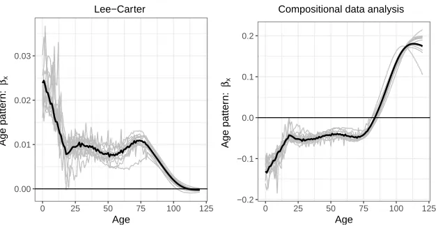
In the methods section, we used similar notation for the parameters of the LC and CoDa models and their coherent versions, as they have similar interpretations but are not iden-tical. The parameters βx, shown in Figure 1, provide an age pattern of the mortality changes. In the LC model, theβxproduce the different rates of mortality improvement by age, when multiplying by the time factorκt. In a CoDa model, this parameter indi-cates the transfer ofdt,xfrom one age to another. The density of deaths for ages where βx are negative will be transferred towards ages whereβx are positive in relative terms (Oeppen 2008).
Figure 1: Age pattern (βx) of the Lee–Carter and CoDa models for the
aver-age (in black) and country-specific (in grey) female mortality of 15 European countries, 1960–2011
0.00 0.01 0.02 0.03
0 25 50 75 100 125
Age
Age patter
n:
βx
Lee−Carter
−0.2 −0.1 0.0 0.1 0.2
0 25 50 75 100 125
Age
Age patter
n:
βx
Compositional data analysis
Source: HMD (2016) and authors’ calculations.
for the CoDa model have more pronounced fluctuations. The coefficient of determination (R2) of a linear regression applied to theκtof the average for each of the models is 99.6% for the LC model and of 97.1% for the CoDa model.
Figure 2: Time index (κt) of the Lee–Carter and CoDa models for the
aver-age (in black) and country-specific (in grey) female mortality of 15 European countries, observed 1960–2011 and forecast 2012–2050
−100 −50 0 50
1975 2000 2025 2050
Year
Time inde
x:
κt
Lee−Carter
−10 0 10 20
1975 2000 2025 2050
Year
Time inde
x:
κt
Compositional data analysis
Fitted Forecast
Source: HMD (2016) and authors’ calculations.
In the CoDa model, the ages with negativeβxrecorded a decrease of their density of deaths over time, in relative terms, once multiplied byκt. They start with adt,xvalue higher than the estimated averageαxand this value decreases over time. Thedt,xbecome smaller thanαxwhenκtcrosses zero. For the ages where theβxare positive, thedt,x is initially lower than the average and then increases over time. In Figures 1 and 2, the density of deaths is thus transferred from younger ages toward older ages.
Lee and Carter (1992) suggest forecastingκtusing a random walk with drift (ARIMA (0,1,0)). We use this procedure to forecast the LCκt. Based on the best BIC value, the κtof the CoDa model is forecast with an ARIMA(0,1,1) model. This model was the one with the best BIC values for most of the selected countries. We here use the same time se-ries for all countse-ries to introduce and compare our model with existing models. However, other time series models could easily be used when forecasting country-specific mortality with CoDa.
country-specific trends,kt,i, should also be forecast. Based on the best BIC values for ARIMA models excluding the use of a drift and moving average (MA) components – i.e., selection between random walk without drift and autoregressive model (AR) as suggested by Li and Lee (2005) – an ARIMA(1,1,0) without drift was selected. This model allows thekt,ito reach a constant while fitting the trends of many countries. This procedure was applied to both LC-coherent and CoDa-coherent models.
4.2 Explained variance and fitted models
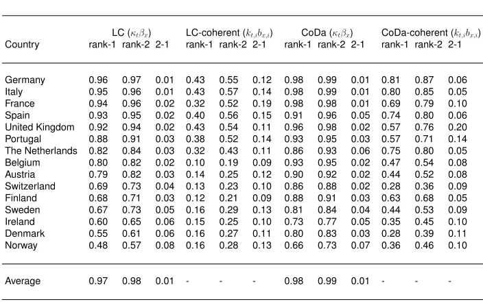
Within a singular value decomposition (SVD), the combination of the first left and right singular vectors and first singular value, called a rank-1 or one-dimensional approxima-tion, is the one explaining the greatest variance. If the explained variance for a rank-1 approximation is low, higher rank approximations can be used. Table 1 presents the ex-plained variance for a rank-1 and rank-2 approximation for the four models and the 15 countries. The Table shows that a rank-1 approximation of the centered matrix of themt,x with the LC model and of thedt,xwith the CoDa model explains most of the variance for most countries. With the CoDa model, a rank-1 approximation explains more than 80% of the variance for 13 out of 15 countries. A rank-2 approximation would increase the explained variance by 7% or less for all countries. Similar results are found for the LC model for most countries. In most cases, no major gains in terms of explained variance would come from adding additional parameters for the second rank in the models. For the coherent models (LC-coherent and CoDa-coherent), the explained variance is lower as it is estimated from themt,xanddt,xmatrices after the common trend has been removed.
The variance explained by the LC model is lower than for the CoDa model for most countries. The errors in modeling and forecasting mortality with the LC and LC-coherent models could then be more important than with the CoDa and CoDa-coherent models.
Table 1: Explained variance of a rank-1 and rank-2 approximation of a sin-gular value decomposition applied within four models, 15 countries and their average, 1960–2011
LC (κtβx) LC-coherent (kt,ibx,i) CoDa (κtβx) CoDa-coherent (kt,ibx,i)
Country rank-1 rank-2 2-1 rank-1 rank-2 2-1 rank-1 rank-2 2-1 rank-1 rank-2 2-1
Germany 0.96 0.97 0.01 0.43 0.55 0.12 0.98 0.99 0.01 0.81 0.87 0.06
Italy 0.95 0.96 0.01 0.43 0.57 0.14 0.98 0.99 0.01 0.80 0.85 0.05
France 0.94 0.96 0.02 0.32 0.52 0.19 0.98 0.98 0.01 0.69 0.79 0.10
Spain 0.93 0.95 0.02 0.40 0.56 0.15 0.91 0.96 0.05 0.74 0.80 0.06
United Kingdom 0.92 0.94 0.02 0.43 0.54 0.11 0.96 0.98 0.02 0.57 0.76 0.20
Portugal 0.88 0.91 0.03 0.38 0.52 0.14 0.93 0.95 0.03 0.57 0.71 0.14
The Netherlands 0.82 0.84 0.03 0.32 0.43 0.11 0.86 0.93 0.06 0.75 0.80 0.05
Belgium 0.80 0.82 0.02 0.10 0.19 0.09 0.93 0.95 0.02 0.47 0.54 0.08
Austria 0.79 0.82 0.03 0.14 0.25 0.12 0.90 0.92 0.02 0.44 0.52 0.08
Switzerland 0.69 0.73 0.04 0.13 0.23 0.10 0.86 0.88 0.02 0.28 0.36 0.09
Finland 0.68 0.71 0.03 0.12 0.21 0.09 0.88 0.91 0.03 0.63 0.68 0.05
Sweden 0.67 0.73 0.05 0.16 0.29 0.13 0.81 0.84 0.04 0.44 0.53 0.09
Ireland 0.60 0.65 0.06 0.15 0.25 0.10 0.73 0.77 0.05 0.35 0.45 0.10
Denmark 0.55 0.61 0.06 0.16 0.27 0.11 0.80 0.83 0.03 0.28 0.39 0.11
Norway 0.48 0.57 0.08 0.16 0.28 0.13 0.66 0.73 0.07 0.36 0.46 0.10
Average 0.97 0.98 0.01 - - - 0.98 0.99 0.01 - -
-Source: HMD (2016) and authors’ calculations.
Note: The countries are listed by order of explained variance obtained with the LC model.
5
Results
5.1 Evaluating the models
lowest MAE average across countries for bothmt,x anddt,x (0.158 and 2.584 respec-tively). This last model would have also performed better than the other models in six and seven countries formt,x anddt,x, respectively. However, the LC-coherent model performs better for seven countries for themt,x, with an average of 0.164.
Table 2: Mean absolute error (MAE) of female logged age-specific death rates (mt,x) over ages and years and the mean Aitchinson distance
(AD) over time for each forecast composition of life table deaths (dt,x)
MAE:mt,x AD:dt,x
Country LC LC-coherent CoDa CoDa-coherent LC LC-coherent CoDa CoDa-coherent
United Kingdom 0.09 0.08 0.10 0.09 1.27 1.22 1.25 1.24
The Netherlands 0.12 0.12 0.12 0.13 1.92 1.94 1.90 1.97
France 0.13 0.11 0.14 0.11 1.69 1.55 1.70 1.53
Germany 0.13 0.14 0.11 0.12 1.91 1.95 1.84 1.88
Italy 0.14 0.16 0.13 0.13 2.09 2.20 2.04 2.09
Spain 0.14 0.15 0.14 0.14 2.15 2.19 2.16 2.13
Belgium 0.14 0.13 0.15 0.14 2.28 2.23 2.26 2.23
Portugal 0.15 0.16 0.14 0.14 2.38 2.41 2.39 2.33
Austria 0.19 0.19 0.17 0.17 2.79 2.78 2.71 2.71
Sweden 0.19 0.18 0.19 0.19 2.97 2.95 2.93 2.88
Finland 0.20 0.19 0.20 0.20 3.21 3.18 3.20 3.17
Norway 0.21 0.20 0.21 0.21 4.12 4.04 4.13 4.12
Switzerland 0.23 0.22 0.23 0.19 3.53 3.44 3.48 3.20
Denmark 0.25 0.20 0.24 0.20 3.68 3.46 3.63 3.44
Ireland 0.25 0.23 0.25 0.22 4.00 3.82 3.91 3.84
Mean 0.17 0.16 0.17 0.16 2.67 2.62 2.63 2.58
No. countries 0 7 2 6 0 4 4 7
Source: HMD (2016) and authors’ calculations.
Note: This table shows the mean absolute error (MAE) of female logged age-specific death rates (mt,x) over ages
and years and the mean Aitchinson distance (AD) over time for each forecast composition of life table deaths for the forecast period 1995–2011, based on the reference period 1960–1994, their average over countries, and number
of countries recording the lowest MAE and AD by model. The countries are listed by order of MAE for themt,x
obtained with the LC model.
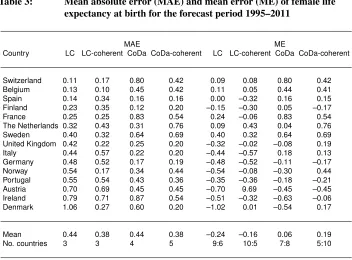
Table 3 presents MAE and the mean error (ME) of female life expectancy at birth forecast for the period 1995–2011, based on the reference period 1960–1994, for 15 coun-tries (see also Appendix E). The MAE is a measure of forecast accuracy while the ME is a measure of bias of the methods. The ME is here defined as:mean[eExpected0 −eObserved
0 ].
would have, in general, increased the accuracy of the forecasts. The coherent version of the CoDa model would have performed better than the other models in 5 out of 15 coun-tries, followed by the CoDa model in 4 countries.
Table 3: Mean absolute error (MAE) and mean error (ME) of female life expectancy at birth for the forecast period 1995–2011
MAE ME
Country LC LC-coherent CoDa CoDa-coherent LC LC-coherent CoDa CoDa-coherent
Switzerland 0.11 0.17 0.80 0.42 0.09 0.08 0.80 0.42
Belgium 0.13 0.10 0.45 0.42 0.11 0.05 0.44 0.41
Spain 0.14 0.34 0.16 0.16 0.00 –0.32 0.16 0.15
Finland 0.23 0.35 0.12 0.20 –0.15 –0.30 0.05 –0.17
France 0.25 0.25 0.83 0.54 0.24 –0.06 0.83 0.54
The Netherlands 0.32 0.43 0.31 0.76 0.09 0.43 0.04 0.76
Sweden 0.40 0.32 0.64 0.69 0.40 0.32 0.64 0.69
United Kingdom 0.42 0.22 0.25 0.20 –0.32 –0.02 –0.08 0.19
Italy 0.44 0.57 0.22 0.20 –0.44 –0.57 0.18 0.13
Germany 0.48 0.52 0.17 0.19 –0.48 –0.52 –0.11 –0.17
Norway 0.54 0.17 0.34 0.44 –0.54 –0.08 –0.30 0.44
Portugal 0.55 0.54 0.43 0.36 –0.35 –0.36 –0.18 –0.21
Austria 0.70 0.69 0.45 0.45 –0.70 0.69- –0.45 –0.45
Ireland 0.79 0.71 0.87 0.54 –0.51 –0.32 –0.63 –0.06
Denmark 1.06 0.27 0.60 0.20 –1.02 0.01 –0.54 0.17
Mean 0.44 0.38 0.44 0.38 –0.24 –0.16 0.06 0.19
No. countries 3 3 4 5 9:6 10:5 7:8 5:10
Source: HMD (2016) and authors’ calculations.
Note: The table shows the mean absolute error (MAE) and mean error (ME) of female life expectancy at birth for the
forecast period 1995–2011, based on the reference period 1960–1994, for 15 countries, their average and number of countries recording the lowest MAE by model or the number of countries with negative vs positive (negative:positive) ME within each model. The countries are listed by order of MAE obtained with the LC model.
above average before the jump-off year (1994). The CoDa-coherent model predicted that the Netherlands’ life expectancy would stay above the average, but it fell behind, an as-pect that the model was not able to anticipate. On the other hand, the model was quite accurate in forecasting the catch-up of Danish females, which started around the jump-off year.
When comparing the accuracy of the two coherent models, LC-coherent and CoDa-coherent, the latter performs better. Using a CoDa-coherent model would have increased the accuracy of the forecast life expectancy for 9 out of 15 countries in comparison with the LC-coherent model (Table 3). However, on average both models have an equal MAE. When looking at the forecast age pattern (Table 2), the CoDa-coherent model would have outperformed the LC-coherent model for 8 and 10 out of 15 countries, for themt,xand dt,x, respectively. As mentioned previously, the CoDa-coherent model has a lower MAE average when estimating the accuracy of the predicted age patterns, both withmt,xand dt,x.
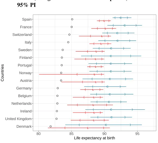
Figure 3 shows the life expectancy forecast with the LC-coherent and CoDa-coherent model in 2011, compared with the observed value. The LC-coherent model underesti-mated the life expectancy of 13 out of 15 countries by the end of the forecast period. The CoDa-coherent model under-predicted the life expectancy of 6 out of 15 countries in 2011 and predicted life expectancy better for 9 countries, in comparison with the LC-coherent model. The prediction intervals (PI) with the CoDa-coherent model are generally wider than with the LC-coherent model. The LC models are generally known to produce very narrow PI (Keilman and Pham 2006). In 2011, the PI of the LC-coherent model con-tains the actual life expectancy at birth for 86.7% of the countries (13/15) for the 95% coverage; and 66.7% (10/15) of the countries for the 80% coverage. However, the CoDa-coherent model might produce PI that are too wide. In 2011, the CoDa-CoDa-coherent model contained the actual life expectancy for 100% (15/15) and 86.7% (13/15) of the countries for the 95% and 80% coverage, respectively.
The CoDa-coherent model produced somewhat more accurate life expectancy and age pattern forecasts for the years 1995 to 2011. However, the CoDa-coherent model tended to overpredict life expectancy in this period, especially the life expectancy of the Netherlands. The noncoherent CoDa model is, however, generally less biased.
5.2 Life expectancy in 2050 5.2.1 More optimistic forecasts
Figure 3: Female life expectancy at birth in 2011 for 15 countries observed and forecast with the LC-coherent and CoDa-coherent models, using 1960–1994 as reference period, and their 80% and 95% PI
CO L C O L C O L C OL C O L C O L C O L C O L C O L CO L C O L C O L C O L C O L C O L ) ) ) ) ) ) ) ) ) ) ) ) ) ) ) ) ) ) ) ) ) ) ) ) ) ) ) ) ) ) ( ( ( ( ( ( ( ( ( ( ( ( ( ( ( ( ( ( ( ( ( ( ( ( ( ( ( ( ( ( Denmark United Kingdom Ireland Netherlands Belgium Germany Austria Norway Portugal Finland Sweden Italy Switzerland France Spain
75 80 85 90
Life expectancy at birth
Countr
ies
O O
O Observed LLL LC-coherent CCC CoDa-coherent
Source: HMD (2016) and authors’ calculations.
Notes: The countries are listed by order of life expectancy observed in 2011.
change in the age-specific death rates from one year to another (see Appendix F for more details on the RMIs) – for the CoDa and CoDa-coherent models can change over time, while they stay constant with the LC and LC-coherent models whenκtis forecast with a random walk with drift, as shown in Appendix F. By using a CoDa methodology, the main LC model problem – i.e., the fixed RMIs (Booth, Maindonald, and Smith 2002; Booth and Tickle 2008; Kannisto et al. 1994) – can then be overcome. As shown in the previous section, the CoDa model is generally less biased. However, the CoDa-coherent model tends to overestimate life expectancy at birth.
previ-Figure 4: Female life expectancy at birth, observed 1960–2011 and forecast 2012–2050 for 15 European countries using four forecasting mod-els
CoDa CoDa-coherent
LC LC-coherent
65 70 75 80 85 90 95
65 70 75 80 85 90 95
1975 2000 2025 2050 1975 2000 2025 2050
Year
Lif
e e
xpectancy at bir
th
Source: HMD (2016) and authors’ calculations.
than negative, or vice versa, the PI bounds might be asymmetric. This is, for example, the case of Norway when forecast with the LC-coherent model.
Figure 5: Female life expectancy at birth for 15 countries, observed in 2011 and forecast in 2050 with the LC-coherent and CoDa-coherent models, using 1960–2011 as reference period, and their 80% and 95% PI C O L C O L C O L C O L C O L C O L C O L C O L C O L C O L C O L C O L C O L C O L C O L ) ) ) ) ) ) ) ) ) ) ) ) ) ) ) ) ) ) ) ) ) ) ) ) ) ) ) ) ) ) ( ( ( ( ( ( ( ( ( ( ( ( ( ( ( ( ( ( ( ( ( ( ( ( ( ( ( ( ( ( Denmark United Kingdom Ireland Netherlands Belgium Germany Austria Norway Portugal Finland Sweden Italy Switzerland France Spain
80 85 90 95
Life expectancy at birth
Countr
ies
O O
OObservedLLLLC-coherentCCCCoDa-coherent
Source: HMD (2016) and authors’ calculations.
5.2.2 Coherence in the forecasts
Figure 6 shows the range (maximum–minimum values) of life expectancy among the se-lected 15 countries. Between 1960 and 2011, the range of life expectancy values decrease from 8.87 years to 3.28 years, mainly due to Portugal catching up with the other countries. Since the 1980s, the range of life expectancy values remains around 3.6 years, confirming the need for coherent forecasting among Western European countries.
Figures 4 and 6 show that adding a common factor to the LC and CoDa models suc-ceeds in reducing the long-term divergence in the forecast life expectancy. For example, under the LC model the difference between the maximum and minimum in the forecast life expectancies in 2050 is 5.77 years, while for the LC-coherent model that gap is 2.68 years. Similar results are found when comparing the CoDa and CoDa-coherent models, with ranges of 5.68 and 2.84 respectively. Using a trend common to Western European countries thus allows one to forecast life expectancy in a more coherent way and avoids increasing divergence in the long term. However, the coherent models predict a further convergence, albeit modest, of life expectancy values even if the range stayed approxi-mately constant in the last three decades.
Figure 6: Range of female life expectancy at birth for 15 European coun-tries, observed from 1960–2011 and forecast from 2012–2050 using four methods
4 6 8 10
1975 2000 2025 2050
Year
Lif
e e
xpectancy range (m
ax−
min)
Observed CoDa-coherent CoDa LC-coherent
LC
6
Discussion
The CoDa methodology is a new forecasting approach and this article is the first to ex-plore its potential to forecast life expectancy coherently among many countries. The results show that using a CoDa-coherent model is a compelling strategy to forecast mor-tality. One important advantage of the model is the changing RMIs over time, which overcomes the problematic fixed RMI assumption of the LC model. This last aspect of the LC model has been criticized for yielding too pessimistic forecasts (Booth, Maindon-ald, and Smith 2002; Kannisto et al. 1994). The noncoherent CoDa methodology allows for more optimistic and less biased forecasts for Western European countries. However, the CoDa-coherent model might sometimes be too optimistic in its forecast.
The changes in the RMIs can come from two aspects of the model: 1) the use of the clrtransformation, which does not produce constant RMI due to the closing procedure C[](see Appendix F); and 2) the use of thedt,xas indicator. Due to the relation between indicators in the life table, modeling an indicator in a certain way might lead to different modeling of other life table indicators, producing different RMIs. More detailed analyses should be performed on the consequences of using different indicators for the forecast results.
Despite somewhat more accurate forecasts, the PI are wider with a CoDa method – suggesting that the forecasts carry more uncertainty – than with an LC method. These results can be considered as inconsistent, but the LC model is known to produce some-what small PI (Keilman and Pham 2006). As mentioned previously, the wider PI from the CoDa models might come from the more pronounced fluctuations of the CoDa time index. The random variation of the respective mortality matrices seems to be captured by κtwith CoDa, but byβxwith the LC model, as shown in Figures 1 and 2. Future research should try to provide a more detailed explanation for these results, look deeper into the causes of the wider PI for CoDa, and consider new ways to estimate the PI.
As mentioned previously, bothkt,i in the LC-coherent and CoDa-coherent are not guaranteed to reach a constant, e.g., if the trend has recorded a long-term increasing or decreasing trend. In this case, the coherent model might fail, as the population’s mortality diverges more and more from the average trend. Mortality for such populations should perhaps not be forecast coherently in the remaining countries. However, in our results such patterns were rarely observed for the selected countries.
shortcomings of the LC model. Oeppen (2008) also showed that this method provides interesting possibilities for forecasting mortality by causes of death.
Further development of the method in different contexts should be the subject of future research, including, among others, cohort forecasts. By reading our results in a cohort perspective, the life expectancy at birth for females born in 1960 in France is pre-dicted to be 88.8 years with the LC-coherent model and 93.1 with the CoDa-coherent model. However, no information on cohort effects has been considered in the models to produce proper cohort forecasts. This could be attained, for example, by adapting the Renshaw and Haberman (2006) model to CoDa.
7
Conclusion
Both LC and CoDa models and their coherent variants (LC-coherent and CoDa-coherent) share some similarities: the parametersβxandκtare found by applying a SVD to a cen-tered matrix and the time index is extrapolated using time series models. However, the models differ in many ways. The key difference is that the forecasts are based on differ-ent indicators: mt,xanddt,x. The use of a specific indicator implies a method adapted to the indicator’s characteristics, as presented earlier. The use of different indicators and methods implies that the parameters have different interpretations and the models have different assumptions. As mentioned previously, the CoDa model is not based on a con-stant RMI assumption, as with the LC model. Furthermore, over time, thedt,x are not free to vary independently from one another, as themt,xcan, an aspect which appears in their covariance structure.
In this article, we forecast mortality acknowledging that there is coherence among Western European countries using compositional data analysis of life table deaths. This procedure is a promising new way to provide a coherent mortality forecast, as it 1) pre-serves coherence among countries, 2) acknowledges covariance between components, 3) explains a large proportion of the observed variability, and 4) allows the rate of mortality improvement to change over time. Our results show that using a CoDa-coherent model to forecast mortality for the period 1995–2011 increased the accuracy of the forecast for many of the selected countries.
8
Acknowledgement
References
Aitchison, J. (1986). The statistical analysis of compositional data. London: Chapman and Hall.
Aitchison, J., Barceló-Vidal, C., Martín-Fernández, J., and Pawlowsky-Glahn, V. (2000). Logratio analysis and compositional distance.Mathematical Geology32(3): 271–275. doi:10.1023/A:1007529726302.
Barbieri, M., Wilmoth, J., Shkolnikov, V., Glei, D., Jasilionis, D., Jdanov, D., Boe, C., Riffe, T., Grigoriev, P., and Winant, C. (2015). Data resource profile: The Human Mortality Database (HMD).International Journal of Epidemiology44(5): 1549–1556. doi:10.1093/ije/dyv105.
Bergeron-Boucher, M.P., Ebeling, M., and Canudas-Romo, V. (2015). Decomposing changes in life expectancy: Compression versus shifting mortality. Demographic Re-search33(14): 391–424.doi:10.4054/DemRes.2015.33.14.
Bohk-Ewald, C. and Rau, R. (2017). Probabilistic mortality forecasting with varying age-specific survival improvements. Genus73(1): 1–37.doi:10.1186/s41118-016-0017-8.
Booth, H., Hyndman, R., Tickle, L., and de Jong, P. (2006). Lee–Carter mortality fore-casting: A multi–country comparison of variants and extensions. Demographic Re-search15(9): 289–310.doi:10.4054/DemRes.2006.15.9.
Booth, H., Maindonald, J., and Smith, L. (2002). Applying Lee–Carter under conditions of variable mortality decline. Population Studies 56(3): 325–336. doi:10.1080/00324720215935.
Booth, H. and Tickle, L. (2008). Mortality modelling and forecasting: A review of meth-ods. Annals of Actuarial Science3(1–2): 3–43. doi:10.1017/S1748499500000440.
Brass, W. (1971). On the scale of mortality. In: Brass, W. (ed.).Biological aspects of demography. London: Taylor and Francis: 69–110.
Cairns, A.J., Blake, D., Dowd, K., Coughlan, G.D., and Khalaf-Allah, M. (2011). Bayesian stochastic mortality modelling for two populations. ASTIN Bulletin41(1): 29–59.doi:10.2143/AST.41.1.2084385.
Camarda, C. (2012). Mortality smooth: An R package for smoothing poisson counts with p-splines.Journal of Statistical Software50(1): 1–24.doi:10.18637/jss.v050.i01.
Egozcue, J.J., Pawlowsky-Glahn, V., Mateu-Figueras, G., and Barcelo-Vidal, C. (2003). Isometric logratio transformations for compositional data analysis. Mathematical Ge-ology35(3): 279–300.doi:10.1023/A:1023818214614.
HMD (2016). Human Mortality Database. [electronic resource]. University of California, Berkeley and Max Planck Institute for Demographic Research. www.mortality.org.
Hyndman, R.J., Booth, H., and Yasmeen, F. (2013). Coherent mortality forecasting: The product-ratio method with functional time series models. Demography50(1): 261– 283.doi:10.1007/s13524-012-0145-5.
Kannisto, V., Lauritsen, J., Thatcher, A.R., and Vaupel, J.W. (1994). Reductions in mor-tality at advanced ages: Several decades of evidence from 27 countries. Population and Development Review20(4): 793–810.
Keilman, N. and Pham, D.Q. (2006).Prediction intervals for Lee–Carter-based mortality forecasts. Paper presented at the European Population Conference 2006, Liverpool, United Kingdom, June 21–24, 2006.
Lee, R.D. (1998). Probabilistic approaches to population forecasting. Population and Development Review24(419): 156–190.doi:10.2307/2808055.
Lee, R.D. and Carter, L.R. (1992). Modeling and forecasting US mortality. Journal of the American Statistical Association87(419): 659–671.
Lee, R.D. and Miller, T. (2001). Evaluating the performance of the Lee–Carter method for forecasting mortality.Demography38(4): 537–549.doi:10.1353/dem.2001.0036.
Li, N. and Lee, R.D. (2005). Coherent mortality forecasts for a group of popu-lations: An extension of the Lee–Carter method. Demography 42(3): 575–594. doi:10.1353/dem.2005.0021.
Lloyd, C.D., Pawlowsky-Glahn, V., and Egozcue, J.J. (2012). Compositional data analy-sis in population studies. Annals of the Association of American Geographers102(6): 1251–1266.doi:10.1080/00045608.2011.652855.
Martín-Fernández, J., Barceló-Vidal, C., and Pawlowsky-Glahn, V. (2003). Dealing with zeros and missing values in compositional data sets using nonparametric imputation.
Mathematical Geology35(3): 253–278.doi:10.1023/A:1023866030544.
Mert, M.C., Filzmoser, P., Endel, G., and Wilbacher, I. (2016). Compositional data analysis in epidemiology. Statistical Methods in Medical Research 1–14. doi:10.1177/0962280216671536.
Swedish Social Insurance Agency: 55–82.
Oeppen, J. (2008). Coherent forecasting of multiple-decrement life tables: A test using Japanese cause of death data. Paper presented at the European Population Conference 2008, Barcelona, Spain, July 9–12, 2008.
Oeppen, J. and Vaupel, J.W. (2002). Broken limits to life expectancy.Science296(5570): 1029–1031.doi:10.1126/science.1069675.
Pawlowsky-Glahn, V. and Buccianti, A. (2011). Compositional data
analysis: Theory and applications. New Jersey: John Wiley. http://www.dx.doi.org/10.1002/9781119976462doi:10.1002/9781119976462.
Pawlowsky-Glahn, V. and Egozcue, J. (2006). Compositional data and their analysis: An introduction.Geological Society264(1): 1–10. doi:10.1144/GSL.SP.2006.264.01.01.
Preston, S., Heuveline, P., and Guillot, M. (2001). Demography: Measuring and model-ing population processes. Oxford: Blackwell.
Raftery, A.E., Chunn, J.L., Gerland, P., and Ševˇcíková, H. (2013). Bayesian proba-bilistic projections of life expectancy for all countries. Demography50(3): 777–801. doi:10.1007/s13524-012-0193-x.
Renshaw, A. and Haberman, S. (2006). A cohort-based extension to the Lee–Carter model for mortality reduction factors. Insurance: Mathematics and Economics38(3): 556–570.doi:10.1016/j.insmatheco.2005.12.001.
Russolillo, M., Giordano, G., and Haberman, S. (2011). Extending the Lee–Carter model: A three-way decomposition. Scandinavian Actuarial Journal2011(2): 96– 117. doi:10.1080/03461231003611933.
Schinzinger, E., Denuit, M.M., and Christiansen, M.C. (2016). A multivariate evolution-ary credibility model for mortality improvement rates. Insurance: Mathematics and Economics69(2): 70–81. doi:10.1016/j.insmatheco.2016.04.004.
Stoeldraijer, L., van Duin, C., van Wissen, L., and Janssen, F. (2013). Impact of dif-ferent mortality forecasting methods and explicit assumptions on projected future life expectancy: The case of the Netherlands. Demographic Research29(13): 323–354. doi:10.4054/DemRes.2013.29.13.
Thatcher, R.A., Kannisto, V., and Vaupel, J.W. (1998). The force of mortality at ages 80 to 120. Odense: Odense University Press.
Torri, T. and Vaupel, J. (2012). Forecasting life expectancy in an
Vaupel, J. and Yashin, A. (1987). Repeated resuscitation: How lifesaving alters life tables.
Demography24(1): 123–135. doi:10.2307/2061512.
White, K.M. (2002). Longevity advances in high-income countries, 1955–1996. Popula-tion and Development Review28(1): 59–76. doi:10.1111/j.1728-4457.2002.00059.x.
Wilmoth, J.R. (1995). Are mortality projections always more pessimistic when dis-aggregated by cause of death? Mathematical Population Studies 5(4): 293–319. doi:10.1080/08898489509525409.
Wilson, C. (2001). On the scale of global demographic convergence 1950– 2000. Population and Development Review 27(1): 155–171. doi:10.1111/j.1728-4457.2001.00155.x.
Wilson, C. (2011). Understanding global demographic convergence since 1950.
Appendix A: CoDa operators and method
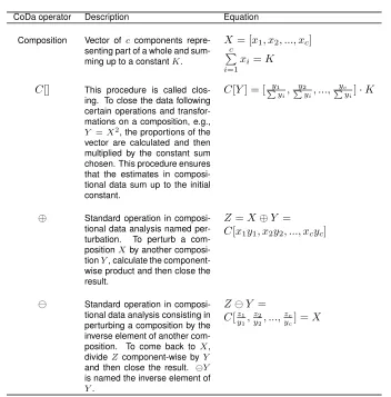
Table A-1 summarizes the different CoDa operators and concepts used in this paper.
Table A-1: CoDa operators and methods used, their descriptions, and equa-tions
CoDa operator Description Equation
Composition Vector of ccomponents
repre-senting part of a whole and
sum-ming up to a constantK.
X = [x1,x2, ...,xc] c
P
i=1
xi=K
C[] This procedure is called
clos-ing. To close the data following certain operations and transfor-mations on a composition, e.g.,
Y =X2, the proportions of the
vector are calculated and then multiplied by the constant sum chosen. This procedure ensures that the estimates in composi-tional data sum up to the initial constant.
C[Y] = [ y1
Py
i,
y2
Py
i, ..., yc
Py
i]·K
⊕ Standard operation in
composi-tional data analysis named
per-turbation. To perturb a
com-positionX by another
composi-tionY, calculate the
component-wise product and then close the result.
Z=X⊕Y =
C[x1y1,x2y2, ...,xcyc]
Standard operation in composi-tional data analysis consisting in perturbing a composition by the inverse element of another
com-position. To come back toX,
divideZ component-wise byY
and then close the result. Y
is named the inverse element of
Y.
Z Y =
C[z1 y1,
z2 y2, ...,
Table A-1: (Continued)
CoDa operator Description Equation
clr() The centered log-ratio (clr)
transformation is one of the
log-ratio representations of
compositional data. This trans-formation is used to represent a composition as a real vector
(U), on which standard
statisti-cal analyses can be used. The
clr-coordinates of a vector X
are the logarithm of the compo-nents divided by its geometric mean.
g= (x1·x2·...·xc)1/c clr(X) = [ln(x1
g ),ln( x2
g), ...,ln( xc
g)]
clr(X) =U
clr−1() The inverseclrtransformation is
the procedure used to re-enter compositional data form,
follow-ing aclrtransformation (fromU
toX). The exponential ofclr
-coordinates are obtained and then closed.
clr−1(U) =C[eu1,eu2, ...,euc]
clr−1(U) =X
AD The Aitchison distance is a
mea-sure of dissimilarity between two
compositions. In this paper,
the AD measure is used as a measure of accuracy between a forecast composition and an ob-served composition. The AD is the square root of the sum of the squared difference between two
compositions expressed in clr
-coordinates.
AD=
c P
i=1
(clr(xi)−clr(yi))2 1/2
Source: Aitchison 1986; Pawlowsky-Glahn and Egozcue 2006; Pawlowsky-Glahn and Buccianti 2011
Additionally, we give here the step-by-step procedure of the CoDa method presented in the main text to forecastdt,x:
2. We obtain a second matrixF, with elementsft,x, by perturbing the matrixDby the column geometric means for each age, αx, by using the CoDa perturbation operator . This step centers the matrix to better visualize the structure:
ft,x=dt,x αx.
3. The next step is to unrestrict the data. Aitchison (1986) showed that compositional data is confined to a restricted space where the components can only vary between 0 and a given limit. Aitchison (1986) suggested using log-ratio transformations to allow the data to vary freely. We here apply the centered log-ratio (clr) transfor-mation:
ht,x=clr(ft,x) =ln( ft,x
gt
), (9)
wheregtare the geometric means over age at timet. We thus obtain a new trans-formed matrix,H, with elementsht,x. This new space, where the data is free to vary from−∞to∞, is known as the “real space.”
4. A singular value decomposition (SVD) is then applied to the matrixH.
5. A low-rank approximation of the matrixH,H∗, is constructed and forecast. Oep-pen (2008) compared a rank-1 and rank-2 approximation of the matrixHand se-lected an ARIMA(0,2,2) model to forecast the time index for Japan, based on the best AIC criterion. In this article, we suggest using a rank-1 approximation of the matrixH, as no major gains in explained variance are obtained, for most countries, by using a rank-2 approximation. The time index is forecast with an ARIMA(0,1,1) model, based on the best BIC value.
6. To transform the matrix back into compositional data, F∗, the inverse centered log-ratio is used:
ft,x∗ =clr−1(ht,x∗ ) =C[eh∗t,x], (10)
whereh∗t,xare the elements of the matrixH∗andC[]is a closing procedure (see Table A-1).
d∗t,x=ft,x∗ ⊕αx. (11)
Appendix B: Prediction intervals
The method used to calculate the prediction intervals (PI) is built on the Keilman and Pham (2006) model and allows us to consider two sources of uncertainty in the forecasts: Estimates of the parameters and extrapolated values of the time index. The following steps apply to the PI of the LC and CoDa models.
1. Estimate the model, extrapolate the time indexκtusing the selected time series model, and construct the matrixκtβx.
2. For each time-age interval, the model provides an error (t,x) (Keilman and Pham 2006). For the CoDa model, the errors are found within the clr transform (see equation (5)). We thus make the hypothesis that the parameterαx, found before theclrtransformation, is correct. The residuals (t,x) are placed in a table. A new table of residuals is created by assigning to each age and year a randomly chosen row and column of the original table. The simulated residuals are added to the fit-ted value,κtβxin step 1. This random allocation procedure is repeatedntimes. For each of thennew tables of values, the model chosen in step 1 is estimated. We thus obtainnestimates ofκtandβx, and take into account the uncertainty in estimating these parameters.
3. For each simulation of step 2, a new time index is found and extrapolated using the selected time series model. At eachnestimate ofκt, PI are estimated using nκsimulations with resampled errors (bootstrap). We obtain a set ofnnκfuture mortality trends. This step considers the uncertainty in the extrapolated value of the time index.
4. For each of thennκ future mortality trends, a life table is calculated. Prediction intervals for age-specific death rates, life table deaths, and life expectancy are ob-tained by finding the 0.025 and 0.975 percentiles of the simulated data for the 95% PI and the 0.1 and 0.9 percentiles for the 80% PI.
for both common and deviation factors, obtainingnnκsimulations for the common fac-tor andndndκ simulation for the deviation term. The errors for the deviation factor at step 2 are found byclr(dt,x αx eκtβx) = kt,ibx,i +t,x,i. For eachnnκ simu-lation of the common factor, we added thend
ndκsimulation for the deviation. We thus obtainnnκndndκsets of future mortality trends. The number of simulations aren=100, nκ=100,nd=100, andndκ=100, leading to a total of 100,000,000 simulations.
Appendix C: Data
Germany
Data for Germany in the HMD is available starting in 1990 only. However, data is avail-able for East and West Germany separately starting in 1956. To obtain longer series for Germany, we combined death counts and exposure to risk data for East and West Germany, taking account of their population size. Life tables for Germany were then calculated starting in 1960.
Average mortality
The average mortality for the 15 selected countries is based on the average of the observed age-specific death rates (m¯t,x):
¯ mt,x=
I P
i=1 mt,x,i
I ,
whereIis the number of countries. These average age-specific death rates weight all the countries equally irrespective of their population size. A life table is then calculated us-ing the average death rates followus-ing standard methods (Preston, Heuveline, and Guillot 2001).
Age 80 to 120 smoothed with a Kannisto model
Vaupel 1998) for old-age mortality and applied it to ages 80 to 120 using a Poisson log-likelihood procedure.
Problems with zeros
When zeros are present in a composition, the log-ratio representation of compositional data is problematic (Martín-Fernández, Barceló-Vidal, and Pawlowsky-Glahn 2003). By applying a Kannisto model to ages 80 to 120, we avoid the problem at old ages. However, for some countries, life table deaths can equal 0 at younger ages for some specific years.
In a life table context, the 0 values occur because no deaths have been observed or counted at a specific age xand timet. Treatment of 0 values is thus done on the observed death counts (Dt,x). Procedures were suggested by Martín-Fernández, Barceló-Vidal, and Pawlowsky-Glahn (2003) to treat zero counts (essential zeros). We use a multiplicative replacement strategy. If we have a compositionXof the observed deaths Dx with P parts, X = [x1,x2, ....,xP], containing zeros, we want to replace it by a composition R with P parts,R= [r1,r2, ....,rP], without zeros:
rj=
δ,
ifxj= 0 (1−zδ
K)xj, ifxj>0
whereδis the imputed value on partxj,zis the number of zeros counted in the compo-sitionX, andKis the constant of the sum constraint (P
xj =K). The value ofδis half of the minimumDt,xobserved over all ages and years, whenDt,x >0, divided by the total number of deaths observed the year the zero was recorded:
δt= min
t,x(Dt,x)/2
120 P
x=0 Dt,x
∀Dt,x>0.
Once the composition R is found, we multiply it by 120 P
x=0
Dt,x to create a new set
Appendix D: The fitted models
Figure A-1 shows the life table deaths for Spanish females, on a log scale, at selected ages (0, 15, 30, 45, 60, 75, 90, and 105) observed and fitted with the LC, LC-coherent, CoDa, and CoDa-coherent models. For most age groups and for all four models, the fit is generally good. The coefficient of determination (R2) value for ages 0, 45, 60, 75, 90, and 105 is 90% and over for all four models. The fit at ages 15 and 30 is however poorer, especially for the CoDa and CoDa-coherent models, withR2 values between 75% and 90%. This value is over 85% with the LC and LC-coherent models at these same two ages. The number of deaths at age 15 and 30 are, however, relatively low, and the errors in modeling and forecasting them will thus have little impact on life expectancy (Lee and Carter 1992). On the other hand, both CoDa models fit the mortality at higher ages very well. The number of deaths at these ages is often important and has been more influential on life expectancy since the second half of the 20thcentury (Bergeron-Boucher, Ebeling, and Canudas-Romo 2015).
Using the coherent version of the LC and CoDa models also moderately increases the fit at some ages. Similar results are found when looking at the model fits for themt,x.
Figure A-1: Life table deaths (dt,x) at specific ages (0, 15, 30, 45, 60, 75, 90,
and 105) with a radix of 1 observed (dot) and fitted (lines) with the LC and CoDa models, as well as their coherent extension, Spanish females, 1960–2011 0 15 30 45 60 75 90 105 0 15 30 45 60 75 90 105 0 15 30 45 60 75 90 105 0 15 30 45 60 75 90 105 CoDa CoDa-coherent LC LC-coherent −8 −6 −4 −8 −6 −4
1960 1980 2000 1960 1980 2000
Year
Log lif
e tab
le deaths
Appendix E: Evaluating the models, all countries
Figure A-2: Female life expectancy at birth observed from 1960 to 2011 (in black) and forecast from 1995 to 2011 for 15 European countries using four forecasting models
CoDa CoDa-coherent LC LC-coherent
75
80
85
75
80
85
75
80
85
75
80
85
75
80
85
A
ustr
ia
Belgium
Denmar
k
Finland
Fr
ance
1960 1970 1980 1990 2000 2010 1960 1970 1980 1990 2000 2010 1960 1970 1980 1990 2000 2010 1960 1970 1980 1990 2000 2010 Year
Lif
e e
xpectancy at bir
Figure A-2: (Continued)
CoDa CoDa-coherent LC LC-coherent
75
80
85
75
80
85
75
80
85
75
80
85
75
80
85
Ger
man
y
Ireland
Italy
Norw
a
y
the Nether
lands
1960 1970 1980 1990 2000 2010 1960 1970 1980 1990 2000 2010 1960 1970 1980 1990 2000 2010 1960 1970 1980 1990 2000 2010 Year
Lif
e e
xpectancy at bir
Figure A-2: (Continued)
CoDa CoDa-coherent LC LC-coherent
75
80
85
75
80
85
75
80
85
75
80
85
75
80
85
P
or
tugal
Spain
Sw
eden
Switz
er
land
United Kingdom
1960 1970 1980 1990 2000 2010 1960 1970 1980 1990 2000 2010 1960 1970 1980 1990 2000 2010 1960 1970 1980 1990 2000 2010 Year
Lif
e e
xpectancy at bir
th
Appendix F: Rates of mortality improvement (RMIs)
The rate of mortality improvement (RMI) at each age implied by the Lee–Carter (LC) model is not supported by empirical findings (e.g., Kannisto et al. 1994). The LC model assumes constant RMIs, while empirical data shows that the RMIs have been increasing, especially at older ages (Kannisto et al. 1994). When using a CoDa model, the RMIs can change over time. The RMI for an indicatorIforecast with a modelM is here defined by:
RM It,xI,M =−I˙t,x It,x
, (12)
where the dot on the top of the variable indicates its derivative with respect to time. For the Lee–Carter model, the RMI calculated for themt,xis equal to
RM It,xm,LC=−κ˙tβx, (13)
whereκ˙tis equal to the drift when forecasting with a random walk with drift: κ˙t = d+t;t= 0. The RMIs for the LC model is thus constant over time, although differing from age to age. When the life table radix is 1, the CoDa model can be rewritten as:
ˆ dt,x=αx
eβxκt Sclr,t
1 Sαt
, (14)
whereSα,tandSclr,tare the sum at timetof the matricesαxC[eκtβx]andeκtβx respec-tively, used in the closure procedure, as
C[eκtβx] = e κtβx
Sclr,t
and
αx⊕C[eκtβx] =
αxC[eκtβx] Sα,t
.
RM It,xd,CoDa= ˙ Sα,t Sα,t
+ ˙ Sclr,t Sclr,t
−κ˙tβx. (15)
As for the LC model,κ˙twith the CoDa model is equal to the drift when forecasting with a random walk with drift, making the term −κ˙tβx a constant. Thus, the terms
˙ Sα,t Sα,t and
˙ Sclr,t
Sclr,t determine ifRM I d,CoDa
t,x is constant or not. To assess howRM I d,CoDa t,x
changes over time, we calculated the RMIs for the forecastdˆt,x, using a random walk with drift to forecastκt. The RMIs for discrete data can be estimated as:
RM It,xI,M =−ln(It+1,x It,x
). (16)
Figure A-3 shows that the RMIs for thedˆt,xforecast with CoDa are not constant over time. The increase of theRM It,xd,CoDaover time is not linear: The increase is accelerating until the middle of the 2030s and then starts to decelerate. The RMIs at each age evolve in parallel and the difference between two consecutive ages is equal to−κ˙t(βx−βx+1). At some ages, the RMI is negative, e.g., 105, meaning that the density of deaths is increasing at these ages.
Figure A-3: Rate of mortality improvement at specific ages for French females’ life table deaths (dt,x) forecast with a CoDa methodology, 2011–
2050
0
15 30,60,75 45
90
105
−0.04 0.00 0.04 0.08
2010 2020 2030 2040 2050
Year
RMI
The RMIs for two different indicators are hard to compare. Thus, from the forecasts of CoDa based ondt,x, age-specific death rates (mt,x) were constructed and their RMIs calculated. Figure A-4 shows the RMIs of themt,xfrom both LC and CoDa models. The figure confirms that the RMIs for the CoDa model are not constant at all ages.
Figure A-4: Rate of mortality improvement at specific ages for French females’ death rates (mt,x) forecast with an LC and CoDa methodology,
2011–2050
0
15
30
45 60 75
90
105
0
15
30
45 60 75
90
105
CoDa LC
0.00 0.02 0.04 0.06 0.08
2010 2020 2030 2040 2050 2010 2020 2030 2040 2050
Year
RMI
Appendix G: Jump-off adjustment
We adjusted the forecasts to correct for the jump-off year level for the CoDa and CoDa-coherent models using the following equation:
djT:T+N,x= ˆdT:T+N,x⊕[dT,x dˆT,x], (17)
whereT is the last year observed,N is the numbers of years forecast anddt,x,dˆt,xand djt,xare the life table deaths observed, fitted, and forecast, and adjusted for the jump-off level, respectively. We use a similar method for the LC and LC-coherent models:
ln(mjT:T+N,x) =ln( ˆmT:T+N,x) + [ln(mT,x)−ln( ˆmT,x)], (18)
wheremt,xare the age-specific death rates at timet. To avoid extrapolating the random variation of the last year observed (T), we smooth it using a P-spline smoothing procedure for Poisson death counts (Camarda 2012).
We also adjusted the PI in such a way that the median of the simulations, used to calculate the PI, is equal to the forecast value for the life expectancy at birth:
B0,tj =B0,t+ (ˆe0,t−M0,t), (19)
whereB0,tis the PI bounds (upper or lower) of the life expectancy at birth at timetand ˆ
e0,tandM0,tare the life expectancy at birth and the median forecasts, respectively. For most cases, the median was very close to the forecast life expectancy.
Furthermore, the forecast ofκt, in some cases, recorded a break in its trend at year T + 1when forecasting with the ARIMA(0,1,1) model due to the MA component. We thus also adjustκtsuch as:
κjT+1:T+n=κT+1:T+n+ [d−(κT+1−κT)] (20)