20
The Determinants of Gini Coefficient in Iran Based on Bayesian Model
Averaging
Mohsen Mehrara
Faculty of Economics, University of Tehran, Tehran, Iran [email protected]
Mojtaba Mohammadian
MSc in Economics, University of Tehran, Tehran, Iran [email protected]
Abstract: This paper has tried to apply BMA approach in order to investigate important influential variables on Gini coefficient in Iran over the period 1976-2010. The results indicate that the GDP growth is the most important variable affecting the Gini coefficient and has a positive influence on it. Also the second and third effective variables on Gini coefficient are respectively the ratio of government current expenditure to GDP and the ratio of oil revenue to GDP which lead to an increase in inequality. This result is corresponding with rentier state theory in Iran economy. Injection of massive oil revenue to Iran's economy and its high share of the state budget leads to inefficient government spending and an increase in rent-seeking activities in the country. Economic growth is possibly a result of oil revenue in Iran economy which has caused inequality in distribution of income.
Keywords: Gini coefficient, Bayesian Model Averaging (BMA).
JEL classifications: H53, C01, I38
1. Introduction
The economic theories on the income distribution entails a vast array of potential factors by which income inequality can be influenced, with little guidance on selection of appropriate variables to include in Gini coefficient regression. The lack of an accepted empirical specification for use in Gini coefficient regression thus generates uncertainty regarding, for example, which explanatory variables must be included in the model, which functional forms are appropriate, or which lag length captures dynamic responses. In econometrics, all these problems are known as problems of model uncertainty (De luca and Magnus, 2011).
Much of the lengthy econometric literature on the subject of model selection is to do estimate large, flexible models and then performing sequence of tests and various restrictions to find a single best model which has all the irrelevant variables omitted (Koop, 2003). Estimating highly flexible models is far from a solution to addressing model uncertainty (e.g. Danilov and Magnus, 2004). It raises concerns about “overfitting” to arrive at specifications
21
This paper sets out a BMA approach to assess how macroeconomic factors affectthe Gini coefficient in Iran during 1976-2010.Section 2 presents a brief review of theoretical and empirical literature on income distribution. We also present the empirical results of the paper in section 3, and section 4 concludes.
2. Theoretical Literature
The primary studies concerning determinants of income inequality investigate the effect of economic growth on income inequality. Argument in this field is started by Kuznets’s
investigation. Kuznets (1955) found an inverted-U shape between per capita income and inequality based on a cross-section of countries:as countries developed, income inequality first increased, peaked, and then decreased. The major driving force was presumed to be structural change that occurred because of labor shifts from a poor and less productive traditional sector to a more productive and differentiated modern sector. Following Kuznets’s study, investigation of 60s and 70s were conducted to test Kuznets’s inverted-U hypothesis based on cross-section of countries. These studies were confirmed Kuznets’s hypothesis (e.g.
Kravis, 1960; Oshima, 1962; Paukert, 1973). But further studies have tested on individual countries challenged Kuznets’sinverted-U hypothesis and evaporated it(e.g. Anand and Kanbor, 1993;Fields, 1989;Deininger and Squire, 1997).
Many studies have been done onother influential factors in Income distribution, including inflation, unemployment, investment, education, government expenditures, taxation, financial development,trade openness and et cetera. In the following we refer to a number of these studies.
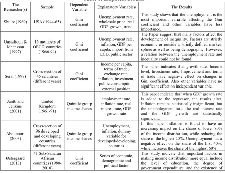
Table 1: Empirical Studies
The Results Explanatory Variables Dependent Variable Sample The Researcher(s)
This study shows that the unemployment is the most important variable affecting the Gini coefficient and other variables have less importance.
Unemployment rate, wholesale price, real GDP growth, trend Gini
coefficient USA (1944-65)
Shultz (1969)
The Paper suggest that many factors affect the development of inequality. Factors are strictly economic or outside a strictly defined market-sphere as well as being demographic. However, a relation between the unemployment rate and inequality could not be found.
Unemployment rate, inflation, GDP per capita, import from LCD, public sector Gini
coefficient 16 members of
OECD countries (1966-94) Gustafsson &
Johansson (1997)
The paper indicates that growth rate, Income level, Investment rate, Improvement and terms of trade have negative effect on changes in Gini coefficient. Also other variables have no significant effect on independent variable. Income per capita,
terms of trade, exchange rate, inflation, investment, public consumption, external position Gini coefficient Cross-section of 45 countries (different years) Seral (1997)
This paper indicate that when GDP growth rate is added to the regressor, the results alter. Inflation remains statistically insignificant, but the unemployment rate, the real interest rate and the GDP growth are statistically significant.
employment rate, inflation rate, real interest rate, GDP
growth rate Quintile group income shares United Kingdom (1961-91) Jantti and Jenkins (2001)
In this paper Inflation is found to have an increasing impact on the shares of lower 80% of the income distribution, while reducing the share of the highest 20%. Unemployment has a negative effect on the share of the first 40%, while increases the share of the highest 60%. Unemployment, inflation, dummy variable for developed/developing countries Quintile group income shares Cross-section of 96 developed and developing countries (different years) Abounoori (2003)
This study indicate that important factors in making income distribution more equal include the level of education, the degree of government expenditure, and the existence of Series of economic,
22
democracy. The Kuznets inverted U- relationship is not supported by the data.
3. Data and Empirical Results
In both theoretical and empirical studies, many different kinds of variables have been considered as significant determinants of Gini coefficient. So in this research, by application of the method of Bayesian Model Averaging (BMA), the effects of influential factors on Gini coefficient which have been regarded in previous studies are investigated.We use Stata program to obtain the coefficient of BMA estimates.
3.1. Data
The variables used in the model arefrom time series data between 1976-2010. All of the data is obtained from Central Bank of Iran (CBI). The variables are regarded based on growth rate and ratio, though all the variables are stationary. Each of variable of model has been presented briefly in Table (2). In advance we concisely explain about some variables of this model.
· The dependent variable is Gini coefficient. Therefore we investigate influential variables on it. The Gini coefficient is the most frequently used indicator of inequality. It is defined as a ratio with values between zero and one in which zero means perfect quality and one means complete inequality.
· The primary studies concerning determinants of income distribution investigate the effect of income level on income inequality. So we use real GDP growth as one of explanatory variable. Also to determine whether income inequality is square root related with economic growth or not, the square of real GDP growth rate is used to examine it.
· Regarding the dependency of Iran to revenue of exported oil and influence of oil revenue on most macroeconomic variables, we consider the ratio of oil revenue to GDP in model.
· Due to importance of education role on income distribution, we use two variables of literacy rate and ratio of the number of public high school student to population (Human capital index) in model.
· One of the subjects discussed in redistribution of incomes is presence of government and its expenditure in economy. Here we include three variables of the ratio of government current expenditure to GDP, the ratio of education department to GDP and the ratio of hygiene and treatment expenditure to GDP in the model in order to investigate their effects on Gini coefficient.
· There are two viewpoints about the relationship between financial development and income distribution. The first viewpoint is argued by Greenwood and Jovanovic (1990), is considered inverse U-shaped relationship between financial development and income inequality. In contrast to the Greenwood-Jovanovic theory, the second viewpoint is assumed a negative linear relationship between these two variables (Banerjee and Newman, 1993; Galor and Zeira, 1993). Accordingly we consider the ratio of M2 (broad money) to GDP and its square as explanatory variables in model to
examine these theories.
23
· We use dummy variable in the model in order to consider the effect of war (1980-1988) on income distribution. This dummy variable adopts one for war years and zero for other years.
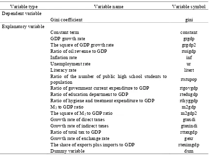
Table 2: List of model’s variables
Variable type Variable name Variable symbol
Dependent variable
Gini coefficient gini
Explanatory variable
Constant term constant
GDP growth rate grgdp
The square of GDP growth rate grgdp2
Ratio of oil revenue to GDP rtoigdp
Inflation rate inf
Unemployment rate ur
Literacy rate litert
Ratio of the number of public high school students to
population rtstupop
Ratio of government current expenditure to GDP rtgovgdp Ratio of education department to GDP rtedugdp Ratio of hygiene and treatment expenditure to GDP rthyggdp
M2 to GDP ratio m2gdp
The square of M2 to GDP ratio m2gdp2
Growth rate of direct taxes gtaxdi
Growth rate of indirect taxes gtaxindi
Ratio of total tax to GDP rttaxgdp
Growth rate of exchange rate gexr
The share of exports plus imports to GDP rteximgdp
Dummy variable dum
3.2. Empirical Results Based on BMA
One of the most important privileges about BMA analyzing is the high level of trust in coefficients estimated in explanatory variables. Because these coefficients are not estimated based on just one model but they are derived from averaging model of estimated coefficients in every single variablewith 262144 (=218) recapitulations or effective samplings.The
coefficient for each of BMA estimates is calculated in this way:
ߚመଵൌ ߣߚመଵ ூ
ୀଵ
ɉ is the possibility of "i" numbers of model and ߚଵ is an estimation ofߚଵ which is gained
24
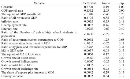
Table 3: The results of BMA estimation
Variable Coefficient t-ratio pip
Constant 0.3720 6.19 1.00
GDP growth rate 0.1312 2.03 0.90
The square of GDP growth rate -0.1202 -0.40 0.20
Ratio of oil revenue to GDP 0.1195 0.85 0.53
Inflation rate 0.0032 0.23 0.11
Unemployment rate 0.0007 0.46 0.23
Literacy rate -0.0283 -0.67 0.40
Raito of the Number of public high school students to
population -0.0738 -0.28 0.20
Ratio of government current expenditure to GDP 0.2092 1.25 0.68 Ratio of education department to GDP -0.0215 -0.25 0.11 Ratio of hygiene and treatment expenditure to GDP -0.5765 -0.54 0.31
M2 to GDP ratio 0.0037 0.08 0.13
The square of M2 to GDP ratio 0.0060 0.17 0.13
Growth rate of direct taxes -0.0060 -0.54 0.29
Growth rate of indirect taxes -0.0007 -0.25 0.11
Ratio of total tax to GDP -0.0116 -0.12 0.11
Growth rate of exchange rate 0.0014 0.22 0.10
The share of exports plus imports to GDP 0.0042 0.29 0.13
Dummy variable 0.0002 0.34 0.17
As a rough guideline for “robustness” of a regressor, a value pip = 0.5 is sometimes
recommended (Raftery, 1995), corresponding approximately with an absolute t-ratio of |t | = 1
(Masanjala and Papageorgiou, 2008). Regarding pip ≥ 0.5 for robustness of a regressor, the results of the table (3) may be explained as follows:
· We see that GDP growth rate is by far the most robust auxiliary regressor with pip = 0.90. It has a positive impact on Gini coefficient. The coefficient of this variable has been obtained 0.13 which indicates that averagely for each percent increase in the economic growth, % 0.13 will be added to the Gini coefficient. Therefore the nature of economic growth in Iran is inclined to more inequality. As a matter of fact, economic growth of Iran is generally in conjunction with oil revenue increase or price perform and liberalization policies which worsen the distribution of income.
· The second effective variable on Gini coefficient is the ratio of government current expenditure to GDP with pip = 0.68.The coefficient of this variable is positive which means an increase in this ratio results in higher degree of inequality. This is probably due to more extensive use of government services by high-income groups of people whereas low-income groups have less chance of using government service. In fact, welfare policies and social spending of government for supporting vulnerable groups has not been efficient.
· The ratio of oil revenue to GDP is the third important auxiliary regressor with pip = 0.53 and it has a positive impact onGini coefficient. Considering economic condition of Iran, oil revenue has an impact on GDP, economic structure and providing the state budget. This result is corresponding with rentier state theory1 in Iran economy. So that interest groups try to possess greater share of oil rents by penetrating into budgeting
1In political science and international relations theory, a rentier state is a state which derives all or a
25
and financial resource allocation. Accordingly it seems oil revenue increase has expanded higher opportunities of rent-seeking and corruption in Iran economy. Besides competitive ability of national products has decreased with increase in availability of foreign exchange resources and more imports of consumption goods and ground is prepared for non-productive and speculative activities and income gap increasing. · Other considered variables have not strong correlation with Gini coefficient with pip
less than 0.5. In fact it seems the other variables have affected the economic inequality from main variables of economic growth, government current expenditure and oil revenue so that after controlling the above variables they have no important effect on Gini coefficient.
3.3. Selection of Optimum Models
"STATA" program present vselect command in order to select variables after performing a linear regression. This command determine the best subsets of each predictor size by using leaps-and-bounds algorithm and provides the five information criteria2 for each of these
models in order to select the optimist model.The optimal model is the one model with these
qualities: the smallest value of Akaike’s information criterion (AIC),Akaike’s corrected
information criterion(AICc) and Bayesian information criterion (BIC); the largest value of R2ADJ (adjusted); and a value of Mallows’s Cp that is close to the number of predictors in the models +1 or the smallest among the other Mallows’s Cp values. These guidelines help avoid
the controversy of which information criterion is the best. Sometimes there is no single model that optimizes all the criteria. There are no fixed guidelines for this situation. Generally, we can narrow the choices down to a few models that are close in optimization (Lindsey and Sheather, 2010). Then we make an arbitrary choice among them. We see the results of vselect command in Table (4):
Table (4): The results of vselect command Optimal Models Highlighted
Preds R2ADJ C AIC AICC BIC
1 .6112954 33.30965 -183.156 -88.67847 -180.163
2 .7417969 13.055 -195.7375 -100.659 -191.248
3 .7781721 8.265046 -199.8671 -103.9949 -193.8811
4 .803071 5.512912 -202.9541 -106.0733 -195.4715
5 .8276937 3.056856 -206.562 -108.432 -197.5829
6 .833581 3.374332 -206.9547 -107.3047 -196.4791
7 .8465719 2.834394 -208.9311 -107.455 -196.959
8 .850569 3.544957 -209.1493 -105.4994 -195.6807
9 .8567865 4.032786 -209.9562 -103.7348 -194.9911
10 .8573041 5.233345 -209.5426 -100.2927 -193.081
11 .8552178 6.722027 -208.5988 -95.79093 -190.6407
12 .8543642 8.061635 -208.0149 -91.03159 -188.5603
13 .8536042 9.383222 -207.5358 -85.65054 -186.5847
14 .8464512 11.292 -205.7457 -78.0958 -183.2981
2An information criterion is a function of a regression model’s explanatory power and complexity. The
26
15 .8389738 13.15531 -204.0629 -69.61293 -180.1188
16 .8301197 15.0552 -202.2971 -59.79001 -176.8565
17 .8194576 17.00375 -200.4181 -48.30662 -173.481
18 .8066135 19 -198.4269 -34.777 -169.9933
Selected Predictors 1: rtoigdp
2: grgdp rtgovgdp 3: grgdp rtgovgdp litert
4: grgdp rtgovgdp grgdp2 litert 5: grgdp rthyggdp rtoigdp gtaxdi litert
6: grgdp rteximgdp rthyggdp rtoigdp dum gtaxdi 7: grgdp rthyggdp gexr ur rtoigdp gtaxdi rtstupop 8: grgdp rthyggdp gexr ur rtoigdp gtaxdi inf rtstupop
9: grgdp rteximgdp rthyggdp gexr ur rtoigdp dum gtaxdi m2gdp2
10: grgdp rteximgdp rthyggdp gexr ur rtoigdp dum gtaxdi m2gdp2 gtaxindi 11: grgdp rteximgdp rthyggdp gexr ur rtoigdp dum gtaxdi inf m2gdp2 gtaxindi
12: grgdp rteximgdp rthyggdp gexr ur rtoigdp dum gtaxdi rtgovgdp grgdp2 inf rttaxgdp 13: grgdp rteximgdp rthyggdp gexr ur rtoigdp dum gtaxdi rtgovgdp grgdp2 inf rttaxgdp rtedugdp
14: grgdp rteximgdp rthyggdp gexr ur rtoigdp dum gtaxdi rtgovgdp grgdp2 inf rttaxgdp rtedugdp
m2gdp2
15: grgdp rteximgdp rthyggdp gexr ur rtoigdp dum gtaxdi rtgovgdp grgdp2 inf rttaxgdp rtedugdp
m2gdp2 gtaxindi
16: grgdp rteximgdp rthyggdp gexr ur rtoigdp dum gtaxdi rtgovgdp grgdp2 inf rttaxgdp rtedugdp litert
m2gdp2 gtaxindi
17: grgdp rteximgdp rthyggdp gexr ur rtoigdp dum gtaxdi rtgovgdp grgdp2 inf rttaxgdp rtedugdp litert
m2gdp2 gtaxindi m2gdp
18: grgdp rteximgdp rthyggdp gexr ur rtoigdp dum gtaxdi rtgovgdp grgdp2 inf rttaxgdprtedugdp litert
m2gdp2 gtaxindi m2gdp rtstupop
Invoking vselect on the data, we find that R2
ADJ and AIC both select the nine-predictor
model. Mallows’sCp advocatesthe eighteen-predictor model when we choose a model with Cp
close to the number ofpredictors +1. Otherwise, when choosing the smallest Cp value, we will
choose the seven-predictor model. The level of difference for each criterion from theAIC-chosen predictor size to its own theAIC-chosen size is minimal. So we choose the seven-predictor model. The optimal model on AICc and BIC is the five-predictor model.
4. Conclusion
27
The results indicate that the GDP growth rate is the most robust auxiliary regressor affecting the Gini coefficient, leading to more inequality. Economic growth is out of favor with low income groups. Thus economic growth policy needs to be revised fundamentally.The second influential factor on Gini coefficient is the ratio of government current expenditure to GDP. The coefficient of this variable is positive which means an increase in this ratio and government interventionworsens the distribution of income. Therefore transfer payments and government expenditure not only failed to achieve one of its rudimentary goals, but also caused more inequality. Also it seems the expenditure is the origin of distribution of rents and corruption and way of its distribution among different groups causes more inequality. The third influential variable on Gini coefficient is the share of oil revenue to GDP which worsens distribution of income. The effect of this variable can happen directly by means of spreading rent-seeking activities or indirectly by means of an increase in imports of consumption goods and decrease of competitive ability of domestic products, reduction of protectionism and the expansion of speculative activity. Other considered variables have not strong correlation with Gini coefficient specially the ratio of M2 to GDP and its square. So this is inconsistent with
Greenwood-Jovanovich theory which assumes inverse U-shaped relationship between financial development and income inequality. Moreover the square of M2 to GDP coefficient
is positive which contrasts to this theory.
5. References
[1] Abounoori, E. (2003). Unemployment, Inflation and Income Distribution: A Cross-country Analysis. Iranian Economic Review (IER), 8(9), 1-11.
[2] Anand, S., & Kanbur, S. R. (1993). Inequality and development a critique. Journal of Development economics, 41(1), 19-43.
[3] Banerjee, A. V., & Newman, A. F. (1993). Occupational choice and the process of development. Journal of political economy, 274-298.
[4] Danilov, D., & Magnus, J. R. (2004). On the harm that ignoring pretesting can cause. Journal of Econometrics, 122(1), 27-46.
[5] De Luca, G., & Magnus, J. R. (2011). Bayesian model averaging and weighted average least squares: Equivariance, stability, and numerical issues. Stata Journal, 11(4), 518. [6] Deininger, K., & Squire, L. (1997). Economic growth and income inequality: reexamining the links. Finance and Development, 34, 38-41.
[7] Fields, G. S. (1989). Changes in poverty and inequality in developing countries. The World Bank Research Observer, 4(2), 167-185.
[8] Galor, O., & Zeira, J. (1993). Income distribution and macroeconomics. The review of economic studies, 60(1), 35-52.
[9] Greenwood, J., & Jovanovic, B. (1990). Financial development, growth, and the distribution of income. The Journal of Political Economy, 98(5), 1076-1107.
[10] Gustafsson, B., & Johansson, M. (1999). In search of smoking guns: What makes income inequality vary over time in different countries?. American Sociological Review, 585-605.
[11] Hopkins, M. (2004). The determinants of income inequality: a Bayesian approach to model uncertainty. Unpublished, Unpublished manuscript, Department of Economics, Gettysburg College, Gettysburg, PA, 76.
[12] Koop, G. (2003).Bayesian Econometrics, John Wiley & Sons Ltd, England.
[13] Kravis, I. B. (1960). International differences in the distribution of income. The Review of Economics and Statistics, 408-416.
28
[15] Lindsey, C., & Sheather, S. (2010). Variable selection in linear regression. Stata Journal, 10(4), 650.
[16] Mahdavy, H. (1970). The pattern and problems of economic development in rentier states: the case of Iran, in Studies in the Economic History of the Middle East, ed. M.A. Cook (Oxford University Press, Oxford 1970).
[17] Masanjala, W. H., & Papageorgiou, C. (2008). Rough and lonely road to prosperity: a reexamination of the sources of growth in Africa using Bayesian model averaging. Journal of Applied Econometrics, 23(5), 671-682.
[18] Oshima, H. T. (1962). The international comparison of size distribution of family incomes with special reference to Asia. The Review of Economics and Statistics, 439-445. [19] Paukert, F. (1973). Income distribution at different levels of development: A survey of the evidence. International Labor Revenue, 108(2), 97-125.
[20] Raftery, A. E. (1995). Bayesian model selection in social research. Sociological methodology, 25, 111-164.
[21] Sarel, M. (1997). How Macroeconomic Factors Affect Income Distribution-The Cross-Country Evidence. International Monetary Fund.
[22] Schultz, T. P. (1969). Secular trends and cyclical behavior of income distribution in the United States: 1944-1965. In Six papers on the size distribution of wealth and income (pp. 75-106). NBER.