Vol. 7, No. 4, 2015 Article ID IJIM-00313, 11 pages Research Article
Numerical solution of two-dimensional fuzzy Fredholm integral
equations using collocation fuzzy wavelet like operator
N. Hassasi ∗, R. Ezzati †‡
————————————————————————————————– Abstract
In this paper, first we propose a new method to approximate the solution of two-dimensional linear fuzzy Fredholm integral equations of the second kind based on the fuzzy wavelet like operator. Then, we discuss and investigate the convergence and error analysis of the proposed method. Finally, to show the accuracy of the proposed method, we present two numerical examples.
Keywords : Fuzzy linear system; Two-dimensional fuzzy Fredholm integral equation; Fuzzy wavelet like operator.
—————————————————————————————————–
1
Introduction
T
hby Dubois and Prade [e concept of fuzzy integrals was initiated11] and then investi-gated by Kaleva [21], Goetschel and Voxman [20], Nanda [25] and others. In [35], the Henstock in-tegral of fuzzy-valued functions is defined, while the fuzzy Riemann integral and its numerical in-tegration was investigated by Wu in [36]. In [17], the authors introduced some quadrature rules for the integral of fuzzy-number-valued mappings. Kaleva [21] proposed the existence and unique-ness of the solution of fuzzy differential equations using the Banach fixed point principle. Mordeson and Newman [24], started the study of the sub-ject of fuzzy integral equations (FIE).Many authors applied the Banach fixed point principle, as a powerful tool, to show the exis-tence and uniqueness of the solution of FIE [5,6,
16, 29, 30, 31]. In [19, 26], sufficient conditions
∗Department of Mathematics, Karaj Branch, Islamic
Azad University, Karaj, Iran.
†Corresponding author. [email protected]
‡Department of Mathematics, Karaj Branch, Islamic
Azad University, Karaj, Iran.
for bounded solutions of FIE are given. Recently, the iterative techniques are applied to solve fuzzy Fredholm integral equations of the second kind (FFIE-2) by researchers [7, 15, 28]. Friedman et al. [16] presented a numerical algorithm to solve FFIE-2 based on successive approximations method. Also, Friedman et al. [17] investigated numerical procedures for solving such equations by using the embedding method. In [8], the suc-cessive approximations method is used for solving nonlinear fuzzy Fredholm integral equations. The authors of [44] presented iterative method and quadrature rules for solving nonlinear FFIE-2. In [9], Bica et al. developed an iterative numerical method to solve fuzzy HammersteVoltera in-tegral equations with constant delay. In [10], the same method has been applied to obtain the solu-tion that take values in the set of right-sided fuzzy numbers for a fuzzy Volterra integral equation with constant delay arising in epidemiology. For numeric-analytic methods to solve FFIE-2, one can refer [1,4,12,13,14,18,27,32,33,34,43]. Since many real-valued problems in engineering and mechanics can be brought in the form of two-dimensional fuzzy Fredholm integral
tions (2DFFIE), it is important that we develop quadrature rules and numerical methods for solv-ing such equations. Recently, some researchers investigated solving such equations. In [?], the authors applied modified Homotopy perturbation method to solve 2DFFIE. The authors of [38] pro-posed quadratur rules for numerical solution of two-dimensional fuzzy integrals. In this work, the authors also obtained numerical solution of linear 2DFFIE by using iterative technique. Also, solv-ing nonlinear 2DFFIE by ussolv-ing quadrature rules is done in [42].
Recently several researchers have attempted to develop ”fuzzy wavelets” based models and sys-tems. Wavelet theory is a relatively new and an emerging area in mathematical research. Also, wavelets are the suitable and powerful tool for approximating functions based on wavelet basis functions. As we know, most of the methods to solve integral equations lead us to solve the lin-ear systems, but the singularity of these systems may cause some problems. So, by using fuzzy wavelet like operator with collocation points to obtain numerical solution of 2FFIE, such linear systems can be as sparse linear systems and it can reduce the cost of computation. In this paper, by using fuzzy wavelet like operator, we propose a numerical method to approximate the solution of linear 2FFIE.
f(x, y) =g(x, y)⊕λ
∫ d
c
∫b
a
K(x, y, s, t)⊗f(s, t)dsdt
(1.1) whereK(x, y, s, t) is an arbitrary kernel function over the square [a, b]×[c, d], andg(x, y) is a fuzzy real valued function ofx and y. Also, we present the error estimation for approximating the solu-tion of equasolu-tion(1.1).
The rest of the paper is organized as follows: In Section2, we review some elementary concepts of the fuzzy set theory and modulus of continuity. In Section5, we present the method for approximate the solution of (1.1) by using fuzzy wavelet like operator. The error estimation of this method is proved in Section 4. Finally in Section 5, we give two numerical examples for applicability of the proposed method and compare the numerical results with the exact solutions.
2
Preliminaries
In this Section, we review some necessary back-grounds and notions of fuzzy sets theory.
Definition 2.1 [3] A fuzzy number is a function
u:R−→[0,1] with the following properties: 1. u is normal, that is ∃x0 ∈ R such that
u(x0) = 1,
2. u is fuzzy convex set
(i.e.u(λx+ (1−λ)y) ≥min{u(x), u(y)} ∀x, y ∈ R, λ∈[0,1]),
3. u is upper semicontinuous on R,
4. The {x∈R:u(x)>0} is compact set.
The set of all fuzzy numbers denoted by RF.
Definition 2.2 [17] Suppose that u ∈ RF. The
r-level set of u is denoted by [u]r = [u(r)− , u+(r)] and is defined by [u]r ={x ∈R;u(x)≥r},where 0 < r ≤ 1. Also,[u]0 is called the support of u
and it is given as [u]0 = {x∈R:u(x)>0}. It follows that the r-level sets of u are closed and bounded intervals in R.
It is well-known that the addition and multiplica-tion operamultiplica-tions of real numbers can be extended toRF. In other words, for u, v∈RF and λ∈R,
we define uniquely the sumu⊕vand the product λ⊗u , by
[u⊕v]r= [u]r+ [v]r, [λ⊗u]r=λ[u]r, ∀r∈[0,1] where [u]r+ [v]r means the usual addition of two intervals ( as subset ofR) andλ[u]r means the usual product between a scalar and a subset of R. We use the same symbol∑both for the sum of real numbers and for the sum⊕( when the terms are fuzzy numbers ).
Definition 2.3 [17] An arbitrary fuzzy number is represented, in parametric form, by an ordered pair of functions (u(r),u¯(r)),0 ≤r≤1, which satisfy the following requirements:
1. u(r) is a bounded left continuous nondecreasing function over [0,1],
2. u¯(r) is a bounded left continuous nonincreasing function over [0,1],
3. u(r)≤u¯(r), 0≤r≤1.
4.The addition and scalar multiplication of fuzzy num-bers inRF are defined as follows:
u⊕v= (u(r) +v(r),u¯(r) + ¯v(r))
λ⊗u= {
(λu(r), λu¯(r)) λ≥0
λu¯(r), λu(r)) λ <0.
Definition 2.4 [3] For arbitrary fuzzy numbers u= (u,u¯)andv= (v,¯v)the quantity
D(u, v) = sup r∈[0,1]
is called the distance betweenuandv. It is shown that
(RF, D)is a complete metric space with the following
properties [7]:
1.D(u⊕w, v⊕w) =D(u, v), ∀u, v, w∈RF, 2.D(k⊗u, k⊗v) =|k|D(u, v), ∀u, v∈RF,∀k∈R, 3.D(u⊕v, w⊕e)≤D(u, w) +D(v, e),∀u, v, e∈RF.
Definition 2.5 [11] Let f, g: [a, b]×[c, d]−→RF be
fuzzy number valued functions. The uniform distance between f andg is defined by
D∗(f, g) = sup{(D(f(x, y), g(x, y));x∈[a, b], y∈[c, d]}.
Definition 2.6 [40] Letf, g : [a, b]×[c, d] −→ RF
. For each partition p = {x1, x2,· · ·, xn}of [a, b]
and q = {y1, y2,· · ·, yn} of [c, d] and for arbitrary
ξi : xi−1 ≤ ξi ≤ xi,2 ≤ i ≤ m and for arbitrary
ηj :yj−1≤ηj ≤yj,2≤j ≤n, let
Rp= m
∑
i=2
n
∑
j=2
f(ξi, ηj)⊗(xi−xi−1)(yj−yj−1).
The function f is called two- dimensional Riemann integrable toI∈RF if for everyϵ >0,
D(I, Rp)< ϵ In this case, we have
I= (F R) ∫ d
c
∫ b
a
f(x, y)dxdy.
Definition 2.7 [42] A function f : [a, b]×[c, d]→
RF is said to be continuous in x0 ∈ [a, b], y0 ∈
[c, d] if for each ϵ > 0 there exist δ > 0 such that
D(f(x, y), f(x0, y0))< ϵ,wheneverx∈[a, b], y∈[c, d]
and√(x−x0)2+ (y−y0)2< δ.We say thatf is fuzzy
continuous on[a, b]×[c, d]if f is continuous at each
(x0, y0)∈[a, b]×[c, d].
The space of all such functions is denoted by
CF([a, b]×[c, d]) .
Lemma 2.1 [40] Iff, g: [a, b]×[c, d]→RF are fuzzy
continuous functions, then the function F : [a, b]× [c, d]→R+ defined by
F(xJy) =D(f(x, y), g(x1y)) is continuous on [a, b], and [c, d]−→R+
defined byF(x, y) =D(f(x, y), g(x, y)) is continuous on [a, b],
and
D((F R)∫cd∫abf(x, y)dxdy,(F R)∫cd∫abg(x, y)dxdy)
≤ ∫ d
c
∫ b
a
D(f(x, y), g(x, y))dxdy.
Definition 2.8 . Let f : [a, b]×[c, d] → RF. One
callfa uniformly continuous fuzzy real number valued function, if and only if for anyϵ >0there existsδ >0
whenever √(x−s)2+ (y−t)2 ≤δ;x, s∈[a, b], y, t∈
[c, d],implies that D(f(x, y)f(s, t)) ≤ ϵ. one denotes it asf ∈CU
F([a, b]).
Definition 2.9 [39] A function f : [a, b]×[c, d] →
RF is said to be bounded if there exist M such that
∥f(x, y)∥F≤ M for any (x, y) ∈ [a, b]×[c, d], where
||f(x, y)||F=D(f(x, y),0) .
Corollary 2.1 [39] If f ∈ CF([a, b] ×[c, d]) , its
definite integral exists [42], furthemore
1. (F R)∫cd∫abf(x, y, r)dxdy=∫cd∫abf(x, y, r)dxdy,
2. (F R)∫cd∫abf(x, y, r)dxdy=∫cd∫abf(x, y, r)dxdy
Remark 2.1 Consider two-dimensional fuzzy Fredholm integral equation of the second kind
f(x, y, r) =g(x, y, r) +λ
∫ d
c
∫b
a
K(x, y, s, t)f(s, t, r)dsdt
In order to design numerical scheme for solving above equation, we first replace it by the system
f(x, y, r) =g(x, y, r) +λ
∫ d
c
∫b
a
K(x, y, s, t)f(s, t, r)dsdt
f(x, y, r) =g(x, y, r) +λ
∫ d
c
∫ b
a
K(x, y, s, t)f(s, t, r)dsdt
where
K(x, y, s, t)f(s, t, r) =
{
K(x, y, s, t)f(s, t, r) K(x, y, s, t)≥0 K(x, y, s, t)f(s, t, r) K(x, y, s, t)<0. K(x, y, s, t)f(s, t, r) =
{
K(x, y, s, t)f(s, t, r) K(x, y, s, t)≥0 K(x, y, s, t)f(s, t, r) K(x, y, s, t)<0. Corollary 2.2 [40] If f, g ∈ RF are Henstock integrale
mappings on [a, b] × [c, d] and if D(f(x, y), g(x, y)) is Lebesgue integrable, then
D((F H)
∫ d
c
∫ b
a
f(x, y)dxdy,(F H)
∫ d
c
∫ b
a
g(x, y)dxdy)
≤(L)
∫ d
c
∫ b
a
D(f(x, y), g(x, y))dxdy.
Definition 2.10 [3] Letf, g: [a, b]×[c, d]→RF
be a bounded function, then function
ω[a,b]×[c,d](f,0) :R+∪ {0} →R+,
ω[a,b]×[c,d] = sup{D(f(x, y), f(s, t))| x, s ∈
where R+ is the set of positive real numbers, is
called the modulus of continuity of f on [a, b]× [c, d].
Some properties of the modulus of continuity are presented below: [7]
1. D(f(x, y), f(s, t))≤
ω[a,b]×[c,d](f,√(x−s)2+ (y−t)2)
,
for anyx, s∈[a, b] andy, t∈[c, d];
2. ω[a,b]×[c,d](f, δ) is increasing function of δ,
3. ω[a,b]×[c,d](f,0) = 0,
4. ω[a,b]×[c,d](f, δ1 + δ2) ≤ ω[a,b]×[c,d](f, δ1) +
ω[a,b]×[c,d](f, δ2) for any δ1, δ2≥0 and
f : [a, b]×[c, d]−→RF,
5. ω[a,b]×[c,d](f, nδ) ≤ nω[a,b]×[c,d](f, δ) for any
δ≥0, n∈N,andf : [a, b]×[c, d]→RF.
6. ω[a,b]×[c,d](f, λδ)≤([λ]+1)ω[a,b]×[c,d](f, δ) for anyδ, λ≥0, and anyf : [a, b]×[c, d]→RF,
where [.] is the ceiling of the number.
In [2], the following theorem is proved.
Corollary 2.3 [2] Let f ϵCF([a, b]× [c, d]) and
the scaling function φ(x, y) a real-valued bounded function with it supp
φ(x, y)⊆[−α, α]×[−β, β],0< α <+∞,0< β < +∞, φ(x, y)≥0 such that
+∞
∑
j=−∞ +∞
∑
i=−∞
φ(x−i)φ(y−j) = 1
on [a, b]×[c, d]. Fork∈Z+, x, y ∈[a, b]×[c, d] , put
(Bkf)(x, y) = +∞
∑
j=−∞ +∞
∑
i=−∞
f( i 2k,
j 2k)⊗
φ(2kx−i)φ(2ky−j) (2.2)
which is a fuzzy-wavelet-like operator. Then
D((Bkf)(x, y), f(x, y))≤ω[a, b]×[c, d](f,
α 2k,
β 2k)
D∗((Bkf), f)≤ω[a,b]×[c,d](f,
α 2k,
β 2k)
for all x, y ∈ R and k ∈ Z+. If f ∈ CFU([a, b]× [c, d]) , then as k → +∞ one gets ω[a,b]×[c,d](f,2αk,
β
2k) → 0 and limk→+∞Bkf = f, point wise and uniformly with rates.
3
Solving
2
FFIE of the second
kind
Here, we use fuzzy wavelet like operator defined by (2.2) due to approximate solution of equation (1.1). To do this, we approximate the solution of (1.1) by (2.2). So, by substituting (2.2) in (1.1) we conclude that
∞ ∑
j=−∞
∞ ∑
i=−∞
f( i 2k,
j
2k)⊗φ(2
kx−i).φ(2ky−j)
∼
=g(x, y) +λ
∫ d
c
∫ b
a
K(x, y, s, t)⊗
∞ ∑
j=−∞
∞ ∑
i=−∞
f( i 2k,
j
2k)⊗(φ(2
ks−i)φ(2kt−j)dsdt (∗)
By using 2ks−i=u and 2kt−j =v, we get
(∗)∼=g(x, y)+
λ 22k
∞ ∑
j=−∞
∞ ∑
i=−∞
f( i 2k
j 2k)⊗
∫ 2kd−j
2kc−j
∫ 2kb−i
2ka−i
K(x, y,u+i 2k ,
v+j
2k )φ(u)φ(v)dudv
(3.3) Now, by using the following scaling function [38]
φ(x, y) = {
1 −12 ≤x, y≤ 12
0 otherwise (3.4)
in (3.3), we conclude that
2kd−1 ∑
j=2kc
2kb−1 ∑
i=2ka
f( i 2k,
j
2k)⊗φ(2
kx−i)φ(2ky−j)∼=
g(x, y) + λ 22k
∑2kd−1 j=2kc
∑2kb−1 i=2kaf(2ik,
j 2k)⊗ ∫ 1
2
−1 2
∫ 1 2 1 2
K(x, y,u+i 2k ,
v+j
2k )φ(u)φ(v)dudv
For fixed k, suppose that
Ai,j,k(x, y) =
λ 22k ∫ 1 2 −1 2 ∫ 1 2 −1 2
K(x, y,u+i 2k ,
v+j 2k )
φ(u)φ(v)dudv,
i= 2ka,2ka+ 1,· · ·,2kb−1,
j= 2kc, 2kc+ 1,· · ·,2kd−1
Clearly, we can write (3.5) in the following form
2kd−1 ∑
j=2kc
2kb−1 ∑
i=2ka
f( i 2k,
j
2k)⊗φ(2 kx
p−i)φ(2kyq−j)
∼
=g(xp, yq)⊕ 2kd−1
∑
j=2kc
2kb−1 ∑
i=2ka
f( i 2k,
j
2k)⊗Ai,j,k(xp, yq)
(3.6) Now, we use collocation points, xp =
p 2k,yq =
q
2k, p= 2
ka,2ka+ 1, . . . ,2kb−1, q= 2kc,2kc+
1· · ·2kd−1 in (3.6). We have:
2kd−1 ∑
j=2kc
2kb−1 ∑
i=2ka
f( i 2k,
j
2k)⊗φ(2 kx
p−i)φ(2kyq−j)
=g(xp, yq)⊕ 2kd−1
∑
j=2kc
2kb−1 ∑
i=2ka
f( i 2k,
j
2k)⊗Ai,j,k(xp, yq)
p= 2ka, 2ka+ 1, . . . , 2kb−1
q = 2kc, 2kc+ 1, . . . , 2kd−1
Thus, we obtain the following 2n×2n, n= 2k(b− a) , fuzzy linear system of equations:
C⊗X=Y ⊕B⊗X,
where
X= (f(a, c), f(a+1 2k, c+
1
2k),· · ·, f(b−
1 2k, d−
1 2k))
t
Y = (g(a, c), g(a+ 1 2k, c+
1
2k),· · ·, g(b−
1 2k, d−
1 2k))
t,
B = (Bi,j)2n×2n, Bij =Ai,j,k(xp, yq),
C = (ci,j)2n×2n, cij =φ(2kxp−i)φ(2kyq−j)
Here, we suppose that b −a ∈ N, d−c ∈ N, where N is set of natural numbers. Clearly, the above system is a dual fuzzy linear system. For solving this system, one can refer to [37]. Finally, by solving this system and using Eq (2.2), we can present the approximate solution of (1.1).
4
Error Estimation
Corollary 4.1 Consider linear 2FFIE of the second kind as follows:
f(x, y) = (g(x, y)⊕λ
∫ d
c
∫ b
a
K(x, y, s, t)⊗f(s, t)dsdt,
where K(x, y, s, t) is an arbitrary continues kernel function having same sign in the square a≤x, s≤b, c≤y, t≤d, andg(x, y)̸= 0 is a con-tinuous fuzzy function over a≤x≤b, c≤y≤d. Under hypothesis of Theorem(2.3) , we have:
D(f(x, y), (Bkf)(x, y))≤M|λ|(b−a)(d−c)
ω[a,b]×[c,d](f, α 2k,
β 2k)
where M = max|K(x, y, s, t)|, a ≤ x, s ≤ b and c≤y, t≤d, and
(Bkf)(x, y) =
∞ ∑ j=−∞ ∞ ∑ i=−∞
f( i 2k,
j 2k)⊗
(φ(2kx−i)φ(2ky−j)
is the approximate solution of equation (1.1). Proof. We would like to estimate
D(f(x, y), (Bkf)(x,y)) =D(g(x, y)⊕
λ
∫ d
c
∫ b
a
K(x, y, s, t)⊗f(s, t)dsdt,
g(x, y)⊕λ∫cd∫abK(x, y, s, t)⊗(Bkf)(s, t)dsdt) =
D(λ
∫ d
c
∫ b
a
K(x, y, s, t)⊗f(s, t)dsdt,
λ
∫ d
c
∫b
a
K(x, y, s, t)⊗(Bkf)(s, t)dsdt) ≤ |λ|
∫ d
c
∫b
a
|K(x, y, s, t)|.D(f(s, t),(Bkf)(s, t))dsdt ≤ |λ|
∫ d
c
∫ b
a
M.D∗(f, Bkf)dsdt ≤
M|λ|(b−a)(d−c)ω[a,b]×[c,d](f,
α 2k,
β 2k)■ It is obvious that
(Bkf)(x, y) =
∞ ∑ j=−∞ ∞ ∑ i=−∞
f( i 2k,
j 2k)⊗
φ(2kx−i)φ(2ky−j)
(Bkf)(x, y) =
∞ ∑ j=−∞ ∞ ∑ i=−∞
f( i 2k,
j 2k)⊗
Now, we consider two cases as follows:
(a)K(x, y, s, t)≥0, (b)K(x, y, s, t)<0. In case (a) , we have:
e=f(x, y)−Bkf)(x, y) = [g(x, y)+
λ
∫ d
c
∫ b
a
K(x, y, s, t)⊗f(s, t)dsdt]− [g(x, y) +λ
∫ d
c
∫ b
a
K(x, y, s, t)(Bkf)(s, t)dsdt]
=λ
∫d
c
∫ b
a
K(x, y, s, t)⊗f(s, t)dsdt−
λ
∫ d
c
∫ b
a
K(x, y, s, t)(Bkf)(s, t)dsdt
=λ
∫d
c
∫ b
a
K(x, y, s, t)[f(s, t)−(Bkf)(s, t)dsdt similary we have:
e=f(s, t)−(Bkf)(s, t)
g(x, y) +λ
∫ d
c
∫ b
a
K(x, y, s, t)f(s, t)dsdt]
−[g(x, y) +λ
∫ d
c
∫ b
a
K(x, y, s, t)(Bkf)(s, t)dsdt].
=λ
∫ d
c
∫ b
a
K(x, y, s, t)f(s, t)dsdt
−λ
∫ d
c
∫ b
a
K(x, y, s, t)(Bkf)(s, t)dsdt
. =λ ∫ d c ∫ b a
K(x, y, s, t)[f(s, t)−Bkf)(s, t)]dsdt
Hence
e=e−e=λ
∫ d
c
∫b
a
K(x, y, s, t)[f(s, t)−(Bkf)(s, t)dsdt
λ
∫ d
c
∫ b
a
K(x, y, s, t)[f(s, t)−(Bkf(s, t)]dsdt
=λ
∫ d
c
∫ b
a
K(x, y, s, t)([f(s, t)−(Bkf)(s, t)])
+[f(s, t)−(Bkf)(s, t)])dsdt,
and
∥e∥=∥e+e∥≤ |λ|
∫d
c
∫ b
a
∥K(x, y, s, t)||[∥f(s, t)−(Bkf)(s, t)∥]
+∥f(s, t)−(Bkf)(s, t)∥]dsdt.]
Since K(x, y, s, t) is an arbitrary continues ker-nel function over the square a ≤ x, s ≤ b, c ≤ y, t ≤ d ,there exist M > 0 such that M = max|K(x, y, s, t)|. So, we can write
∥e∥≤ |λ|M
∫ d
c
∫ b
a
[∥f(s, t)−(Bkf)(s, t)∥
+∥f(s, t)−(Bkf)(s, t)∥]dsdt. (4.7)
On the other hand, we have:
f(s, t)−Bkf(s, t) =f(s, t)
∞ ∑ j=−∞ ∞ ∑ i=−∞
φ(2kx−i)φ(2ky−j)−
∞
∑
j=−∞ ∞
∑
i=−∞
f( i 2k,
j 2k)⊗φ(2
k
x−i)φ(2ky−j)
=
∞
∑
j=−∞ ∞
∑
i=−∞
[f(s, t)−f( i 2k,
j 2k)]φ(2
k
x−i)(p(2ky−j),
Therefore
∥f(s, t)−(Bkf)(s, t)∥=
∞ ∑ j=−∞ ∞ ∑ i=−∞
[f(s, t)−f( i 2k,
j 2k)]
φ(2kx−i)(φ(2ky−j)∥
≤ ∑∞ j=−∞
∞
∑
i=−∞
∥f(s, t)−f( i 2k,
j 2k)]∥φ(2
k
x−i)(φ(2ky−j)
≤ ∑∞ j=−∞
∞
∑
i=−∞
ω[f∥x− i 2k, y−
j 2k∥]
φ(2kx−i)(φ(2ky−j), (∗∗)
Notice that, under hypotheses of Theorem (2.3), we conclude that
−α≤2kx−i≤α⇒ −α 2k ≤x−
i 2k ≤
α 2k
⇒ |x− i 2k|≤
α 2k,
−β≤2kx−i≤β ⇒ −β
2k ≤x−
i 2k ≤
β 2k
⇒ |x− i 2k|≤
β 2k.
Hence
(∗∗)≤
∞
∑
j=−∞ ∞
∑
i=−∞
φ(2kx−i)φ(2ky−j)
ω[a,b]×[c,d]( ¯f ,
α 2k,
β
2k) =ω[a,b]×[c,d]( ¯f ,
α 2k,
β 2k) Therefore, as k→+∞ we get
∥f(s, t)−(Bkf)(s, t)∥→0
Similarly, we conclude
So we obtain that
∥e||=∥e+e∥→0,
as k→+∞.
In case (b) we have K(x, y, s, t)<0. So
e= [g(x, y) +λ
∫ d
c
∫ b
a
K(x, y, s, t)f(s, t)dsdt
−[g(x, y) +λ
∫ d
c
∫ b
a
K(x, y, s, t)(Bkf)(s, t)dsdt]
= +λ
∫ d
c
∫ b
a
K(x, y, s, t)(f(s, t)−Bkf)(s, t)dsdt
and similarly way, we have:
e=λ
∫ d
c
∫ b
a
K(x, y, s, t)[f(s, t)−(Bkf)(s, t)]dsdt
Hence
∥e∥=∥e+e∥
≤ |λ|M
∫ d
c
∫ b
a
∥K(x, y, s, t)∥[∥f(s, t)−(Bkf)(s, t)∥+
∥f(s, t)−(Bkf)(s, t)∥]dsdt
≤ |λ|M(b−a)(d−c)[ω[a,b]×[c,d](f , α 2k,
β bk)
+ω[a,b]×[c,d](f ,
α 2k,
β 2k)
Clearly, we have:
∥e∥=∥e+e∥→0,as k→+∞.
5
Numerical examples
To illustrate the efficiency of the presented method in Section , we give two examples. Also, we compare the numerical solutions obtained by using the proposed method with the exact solu-tions. Trough this section, we suppose that
φ(x, y) = {
1 −12 ≤x, y≤ 12 0otherwise
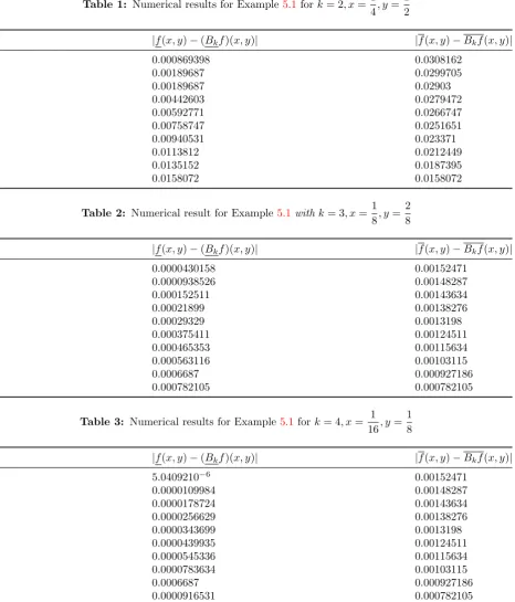
Example 5.1 Consider the following linear 2FFIE of the second kind
g(x, y, r) = (x.siny 2)(r
2+r)
g(x, y) = (x.siny 2)(4−r
3−r)
K(x, y, s, t) =x2ys; 0≤x, y, s, t≤1
Also, let a=o, b= 1. The exact solution of this example is given by
f(x, y, r) = [(x.siny 2)−
16 21(cos
1 2−1).x
2y](r2+r)
f(x, y, r) = [(x.siny 2)−
16 21(cos
1 2−1).x
2y](4−r3−r)
By using the proposed method in Section 5, we can present the approximate solution for this ex-ample. To compare the numerical results with the exact solution for different values of x, y and k, see Tables 1-3.
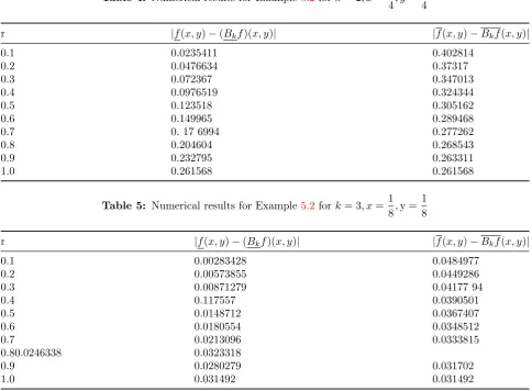
Example 5.2 Consider the following linear 2FFIE ofthe second kind
g(x, y, r) =r(1 3r+
8
3)(1 +x+y− 7 12xy)
g(x, y) = (2r2−4r+ 5)(1 +x+y− 7 12xy) K(x, y, s, t) =xyst; 0≤x, y, s, t≤1
Also, let a= 0, b= 1. The exact solution of this example is given by
f(x, y, r) =r(1 3r+
8
3)(x+y+ 1)
f(x, y, r) = (2r2−4r+ 5)(x+y+ 1)
By using the proposed method in Section 5, we can present the approximate solution for this ex-ample. To compare the numerical results with the exact solution for different values of x, y and k, see Tables 4-5.
6
Conclusion
Table 1: Numerical results for Example5.1fork= 2, x= 1 4, y=
1 2
r |f(x, y)−(Bkf)(x, y)| |f(x, y)−Bkf(x, y)|
0.1 0.000869398 0.0308162
0.2 0.00189687 0.0299705
0.3 0.00189687 0.02903
0.4 0.00442603 0.0279472
0.5 0.00592771 0.0266747
0.6 0.00758747 0.0251651
0.7 0.00940531 0.023371
0.8 0.0113812 0.0212449
0.9 0.0135152 0.0187395
1.0 0.0158072 0.0158072
Table 2: Numerical result for Example 5.1withk= 3, x= 1 8, y=
2 8
r |f(x, y)−(Bkf)(x, y)| |f(x, y)−Bkf(x, y)|
0.1 0.0000430158 0.00152471
0.2 0.0000938526 0.00148287
0.3 0.000152511 0.00143634
0.4 0.00021899 0.00138276
0.5 0.00029329 0.0013198
0.6 0.000375411 0.00124511
0.7 0.000465353 0.00115634
0.8 0.000563116 0.00103115
0.9 0.0006687 0.000927186
1.0 0.000782105 0.000782105
Table 3: Numerical results for Example 5.1fork= 4, x= 1 16, y=
1 8
r |f(x, y)−(Bkf)(x, y)| |f(x, y)−Bkf(x, y)|
0.1 5.0409210−6 0.00152471
0.2 0.0000109984 0.00148287
0.3 0.0000178724 0.00143634
0.4 0.0000256629 0.00138276
0.5 0.0000343699 0.0013198
0.6 0.0000439935 0.00124511
0.7 0.0000545336 0.00115634
0.8 0.0000783634 0.00103115
0.9 0.0006687 0.000927186
1.0 0.0000916531 0.000782105
References
[1] S. Abbasbandy, E. Babolian, M. Alavi, Nu-merical method for solving linear fredholm fuzzy integral equations of the second kind, Chaos Solutions an Fractals 31 (2007) 138-146.
[2] R. Ezzati, F. Mokhtarnejad, N. Hassasi, Some fuzzy-wavelet-like operators and their
convergence, Mathematical Problems in En-gineering (2013), Article ID 832831, 10 pages,http://dx.doi.org/10.1155/2013/ 832831/.
[3] G. A. Anastassiou, Fuzzy mathematics: Ap-proximation theory, Springer-Verlag Berlin Heidelberg (2010).
Ab-Table 4: Numerical results for Example5.2fork= 2, x= 1 4, y=
1 4
r |f(x, y)−(Bkf)(x, y)| |f(x, y)−Bkf(x, y)|
0.1 0.0235411 0.402814
0.2 0.0476634 0.37317
0.3 0.072367 0.347013
0.4 0.0976519 0.324344
0.5 0.123518 0.305162
0.6 0.149965 0.289468
0.7 0. 17 6994 0.277262
0.8 0.204604 0.268543
0.9 0.232795 0.263311
1.0 0.261568 0.261568
Table 5: Numerical results for Example5.2fork= 3, x= 1 8,y =
1 8
r |f(x, y)−(Bkf)(x, y)| |f(x, y)−Bkf(x, y)|
0.1 0.00283428 0.0484977
0.2 0.00573855 0.0449286
0.3 0.00871279 0.04177 94
0.4 0.117557 0.0390501
0.5 0.0148712 0.0367407
0.6 0.0180554 0.0348512
0.7 0.0213096 0.0333815
0.80.0246338 0.0323318
0.9 0.0280279 0.031702
1.0 0.031492 0.031492
basbandy,Numerical solution of linear Fred-holm fuzzy integral equations of the second kind by Adomin method, Appl. Math. Com-put. 161 (2006) 733-744 .
[5] K.Balachandran, K. Kanagarajan,Existence of solutions general nonlinear fuzzy Volterra-Fredholm integral equations, Appl. Math. Stochastic Anal. 3 (2005) 333-343.
[6] K. Balachandran, P. Prakash, Existence of solutions of nonlinear fuzzy Volterra-Fredholm integral equations, Indian J. Pure Appl. Math. 33 (2002) 329-343.
[7] B. Bede, S. G. Gal, Quadrature rules for integrals of fuzzy-number-valued functions, Fuzzy Sets and Systems 145 (2004) 359-380.
[8] A. M. Bica, Error estimation in the approx-imation of the solution of nonlinear fuzzy Fredholm integral equations, Information Sci-ences 178 (2008) 1279-1292.
[9] A. M. Bica, C. Popescu, Numerical solu-tions of the nonlinear fuzzy Hammerstein-Volterra delay integral equations, Informa-tion Sciences 223 (2013) 236-255.
[10] A. M. Bica, One-sided fuzzy numbers and applications to integral equations form epi-demiology, Fuzzy Sets and Systems 219 (2013) 27-48.
[11] D. Dubois, H. Prade, Towards fuzzy differ-ential calculus, Fuzzy Sets and Systems 8 (1982) 1-7.
[12] R. Ezzati, S. Ziari, Numerical solution and error estimation of fuzzy Fredholm integral equation using fuzzy Bernstein polynomials, Aust. J. Basic Appl. Sci. 5 (2011) 2072-2082.
[14] M. Friedman, M. Ma, A. Kandel, Numerical methods for calculating the fuzzy integral, Fuzzy Sets and Systems 83 (1996) 57-62.
[15] M. Friedman, M. Ma, A. Kandel, On fuzzy integral equations, Fund. Inform. 37 (1999) 89-99.
[16] M. Friedman, M. Ma, A. Kandel, Solutions to fuzzy integral equations with arbitrary ker-nels, International Journal of Approximate Reasoning 20 (1999) 249-262.
[17] M. Friedman, M. Ma, A. Kandel, Numer-ical solutions of fuzzy differential and inte-gral equations, Fuzzy Sets and Systems 106 (1999) 35-48.
[18] S. Ziari, R. Ezzati, S. Abbasbandy, Numeri-cal solution of linear fuzzy Fredholm integral equations of the second kind using fuzzy Haar wavelets, Commun. Comput. Inf. Sci. 299 (3) (2012) 79-89.
[19] D. N. Georgiou, I. E. Kougias, Bounded so-lutions for fuzzy integral equations, Int. J. Math. Math. Sci. 31 (2002) 109-114.
[20] R. Goetschel, W. Voxman,Elementary fuzzy calculus, Fuzzy Sets and Systems 18 (1986) 31-43. O. Kaleva, Fuzzy differential equa-tions, Fuzzy Sets and Systems 24 (1987) 301-317.
[21] J. Mordeson, W. Newman, Fuzzy integral equations, Inform. Sci. 87 (1995) 215229.
[22] S. Nanda,On integration of fuzzy mappings, Fuzzy Sets and Systems 32 (1989) 95-101.
[23] J. J. Nieto, R. Rodriguez-Lopez, Bounded solutions for fuzzy differential and integral equations, Chaos Solitons Fractals 27 (2006) 1376-1386.
[24] N. Parandin, M. A. Fariborzi Araghi, The numerical solution of linear fuzzy Fredholm integral equations of the second kind by using finite and divided differences methods, Soft Computing 15 (2010) 729-741.
[25] J. Y. Park, S. Y. Lee, J. U. Jeong, The ap-proximate solution of fuzzy functional inte-gral equations, Fuzzy Sets and Systems 110 (2000) 79-90.
[26] J. Y. Park, J. U. Jeong, On the existence and uniqueness of solutions of fuzzy Volttera-Fredholm integral equations, Fuzzy Sets and Systems 115 (2000) 425-431.
[27] J. Y. Park, J. U. Jeong, A note on fuzzy integral equations, Fuzzy Sets Systems 108 (1999) 193-200.
[28] J. Y. Park, H. K. Han,Existence and unique-ness theorem for a solution of fuzzy Volterra integral equations, Fuzzy Sets Systems 105 (1999) 481-488.
[29] A. Jafarian, S. Measoomy Nia, S. Tavan, A numerical scheme to solve fuzzy linear Volterra integral equations system, Journal of Applied Mathematics (2012) Article ID 216923, 17 pages http://dx.doi.org/doi: 10.1155/2012/216923/.
[30] H. Sadeghi Goghary, M. Sadeghi Goghary, Two computational methods for solving lin-ear Fredholm fuzzy integral equations of the second kind by Adomian method, Appl. Math. Comput. 161 (2005) 733-744.
[31] M. Shafiee, S. Abbasbandy, T. Allahviran-loo, Predictor-corrector method for nonlin-ear fuzzy Volterra integral equations, Aust. J. Basic Appl. Sci. 5 (2011) 2865-2874.
[32] C. Wu, Z. Gong, On Henstock integral of fuzzy-number-valued functions, Fuzzy Sets and Systems 120 (2001) 523-532.
[33] H. C. Wu, The fuzzy Riemann integral and its numerical integration, Fuzzy Sets and Systems 110 (2000) 1-25.
[34] M. Friedman, M. Ming, A. Kandel, Fuzzy linear systems, Fuzzy Sets and Systems 96 (1998 ) 201- 209.
[35] G. A. Anastassiou, Fuzzy wavelet type op-erators, Nonlinear Functional Analysis and Applications 9 (2004) 251 269.
[37] S. M. Sadatrasoul, R. Ezzati, Quadrature Rules and Iterative Method for Numerical Solution of Two-Dimensional Fuzzy Integral Equations, (2014) Article ID 413570.
[38] F. Mokhtarnejad, R. Ezzati, Existence and uniqueness of the solution of fuzzy-valued in-tegral equations of mixed type, Iranian Jour-nal of Fuzzy Systems 12 (2015) 87-94.
[39] R. Ezzati, S. Ziari, Numerical Solution of Two-Dimensional Fuzzy Fredholm Integral Equations of the Second kind Using Fuzzy Bivariate Bernestein Polynomials, Fuzzy Sets and Systems 15 (2013) 84-89.
[40] S. M. Sadatrasoul, R. Ezzati, Itera-tive method for numerical solution of two-dimensional nonlinear fuzzy in-tegral equations, Fuzzy Sets Syst. 12 (2014)http://dx.doi.org/doi: 10.1016/j.fss.2014.12.008.
[41] M. Baghmisheh, R. Ezzati, Numerical solu-tion of fuzzy Fredholm integral equasolu-tions of the second kind using hybrid of block-pulse functions and Taylor series, Advances in Dif-ference Equations (2015) http://dx.doi. org/doi:10.1186/s13662-015-0389-7/.
[42] R. Ezzati, S. Ziari, Numerical solution of nonlinear fuzzy Fredholm integral equations using iterative method, Appl. Math. Com-put. 225 (2013) 33-42.
[43] F. Mokhtarnejad, R. Ezzati, The numerical solution of nonlinear Hammerstein fuzzy in-tegral equations by using fuzzy wavelet like operator, Journal of Intelligent and Fuzzy Systems 28 (2015) 1617-1628.
[44] S. M. Sadatrasoul, R. Ezzati, Numerical so-lution of two-dimensional nonlinear Ham-merstein fuzzy integral equations based on optimal fuzzy quadrature formula, Journal of Computational and Applied Mathematics 292 (2016) 430-446.
Nader Hassasi was born in Marand, Iran in 1974. He received his B.S. degree in Teaching Math-ematics in 1997 from Marand Branch Islamic Azad University, and M.S. in 1999 from Lahijan Branch Islamic Azad University. He is currently the member of board at the IAU-Malayer Branch where he is a Scientific Club member since (2007). Since 2011 he is Ph.D research student in Numerical Analysis at Islamic Azad University, Karaj Branch, Iran. His main research interest is fuzzy mathematics especially, on numerical solution of fuzzy integral equations.