A Modified Degenerate Kernel Method for the System of Fredholm Integral Equations of the Second Kind

(1)

Vol. 14, No. 1 (2019), pp 43-53 DOI: 10.7508/ijmsi.2019.01.005

A Modified Degenerate Kernel Method for the System of

Fredholm Integral Equations of the Second Kind

Ahmad Molabahrami

Department of Mathematics, Ilam University, PO Box 69315516, Ilam, Iran. E-mail: [email protected]

Abstract. _{In this paper, the system of Fredholm integral equations of} the second kind is investigated by using a modified degenerate kernel method (MDKM). To construct a MDKM the source function is approxi-mated by the same way of producing degenerate kernel. The interpolation is used to make the needed approximations. Lagrange polynomials are adopted for the interpolation. The equivalency of proposed method and Lagrange-collocation method is shown. The error and convergence analy-sis of the algorithm are given strictly. The efficiency of the approach will be shown by applying the procedure on some prototype examples.

Keywords: A system of Fredholm integral equations of the second kind, De-generate kernel method, A modified deDe-generate kernel method, Lagrange in-terpolation method, Lagrange-collocation method.

2000 Mathematics subject classification: 45B05.

1. Introduction

The solutions of integral equations have a major role in the fields of science and engineering. A physical event can be modeled by the differential equa-tion (ODE/PDE), an integral equaequa-tion (IE) or an integro-differential equaequa-tion

Received 24 April 2016; Accepted 15 February 2017 c

2019 Academic Center for Education, Culture and Research TMU

43

(2)

(IDE) or a system of these [10]. In this study, we consider the system of Fred-holm integral equations of the second kind of the form [14]

ui(x) =fi(x) + ri X j=1

λij Z b

a

Kij(x, t, u(t))dt, i= 1,2, ..., m, (1.1)

where x _∈ [a, b], λij is a parameter, fi(x) is the source (or data) function, Kij is the kernel function, u(t) = (u1(t), ..., um(t)) and ui(x), i = 1,2, ..., m, are the unknown functions that will be determined. For the linear case, it is assumed that Kij(x, t, u(t)) =Pm_r=1γijrkijr(x, t)ur(t). We rewrite Eq. (1.1) in the matrix form as follows

u(x) =f(x) + Z b

a

K(x, t, u(t))dt, (1.2) where

f(x) = (f1(x), ..., fm(x))T ,

K(x, t, u(t)) = (k1, ..., km)T_,

ki = ri P j=1

λijKij(x, t, u(t)), i= 1,2, ..., m.

There are several analytical and numerical methods for solving integral equa-tions, such as homotopy methods [4, 14, 6], an iterative method [3], a matrix based method [5] and differential transform method [15].

In this paper, a review of degenerate kernel is given. Then we introduce a mod-ified of degenerate kernel method by approximating source function using the same way of producing degenerate kernel. We use the Lagrange interpolation method to obtain the needed approximations and we show that for this case the modified degenerate kernel method is equivalent to the Lagrange-collocation method. The error and convergence analysis of the modified degenerate kernel method are given strictly.

2. The Degenerate Kernel Method

The degenerate kernel method (DKM) is a well-known classical method for solving Fredholm integral equations of the second kind, and it is one of the easiest numerical methods to define and analyze [1, page 23]. This method for a given degenerate kernel is called direct computation method (DCM) [11] and [16, page 141].

We work in the space X = C[a, b] with k · k∞. We define the the integral

operatorK of (1.2) as follows

K[u(x)] = Z b

a

K(x, t, u(t))dt. (2.1)

(3)

For the linear case, the integral operator denoted by (2.1) reduces as follows

Ku(x) = Z b

a

K(x, t)u(t)dt. (2.2) The integral operatorKis assumed to be a compact operator onX into X. The kernel functionK is approximated as follows

Kn(x, t, u(t)) = n X i=1

φi(x)ψi(t, u(t)), (2.3) such that the associated integral operatorsKn satisfy

lim

n_→+∞kK − Knk= 0. (2.4)

Generally, we prefer this convergence to be rapid to obtain rapid convergence of un, touwhereunis the solution of the approximating equationun_−Kn[un] =f. For this purpose, for linear case, we first outline a theorem as already given in [1, page 24, Theorem 2.1.1]. Then, we extend the mentioned theorem for the nonlinear case.

Theorem 2.1. Assume 1− K : X −−→1−1

into X, with X a Banach space and K

bounded. Further, assume _Kn is a sequence of bounded linear operators with (2.4). Then

1. Then the operators(1− Kn)−1 _{exist from}_X _onto_X _{for all sufficiently}

largen, sayn≥N, and

(1− Kn)

−1 6

(1− K)

−1 1−

(1− K)

−1

kK − Knk

, n>N.

2. For the equationsu− K[u] =f andun− Kn[un] =f,n≥N, we have

ku−unk ≤

(1− Kn)

−1

kKu− Knuk (2.5)

Proof. Refer to [1] by settingλ= 1.

Remark 2.2. In using piecewise polynomial interpolation with polynomials of degreeP >0, it is straightforward to show that the errorku−unk∞isO(hP+1)

providedK(x, t) andu(x) are sufficiently differentiable [1, page 41]. Now, we extend Theorem 2.1 for the nonlinear case.

Theorem 2.3. Assume _K is bounded. Further, assume _Kn is a sequence of

bounded operators with (2.4) andKsatisfies uniform Lipschitz condition

kK[u]− K[un]k∞≤LKku−unk∞, (2.6) where L_K _≥ 0 and 1−L_K > 0. Thus, for the equations u_{− K}[u] = f and

un− Kn[un] =f, we have

ku−unk_∞6 K˜n

1−L_K, (2.7)

(4)

where_K˜n=kK[un]− Kn[un]k_∞.

Proof. We have

u₋un =K[u]− K[un] +K[un]− Kn[un], therefore

ku−unk∞≤LKku−unk∞+ ˜Kn,

this ends the proof.

Remark 2.4. From (2.4) and (2.7), we find that ifkK − Knkconverges rapidly to zero, then the same is true ofku−unk_∞.

2.1. Solution of DKM. DKM transforms a Fredholm integral equation of the second kind to a system of algebraic equations. To handle Eq. (1.2), by using DKM, we can express the procedure as follows

1. Substituting (2.3) into (1.2) gives un(x;α) =f(x) +

n X i=1

αiφi(x), (2.8)

where

αi= Z b

a

ψi(t, u(t))dt, i= 1, ..., n, (2.9) andα= (α1, ..., αn).

2. Replacing Eq. (2.8) into (2.9) leads to the following algebraic system

αi= Z b

a ψi



t, f(t) + n X j=1

αjφj(t) 

dt, i= 1, ..., n. (2.10) 3. Solving Eq. (2.10) provides values of αi, i = 1, ..., n, for substituting

them into the Eq. (2.8) to obtain solution of Eq. (1.2).

Remark 2.5. In [1, page 26, Theorem 2.1.2], under some assumptions, it was shown that the linear form of the algebraic system (2.10) is nonsingular.

3. The Modified Degenerate Kernel Method

The modified degenerate kernel method (MDKM) is obtained by approx-imating source function using the same way of producing degenerate kernel denoted by Eq. (2.3) [11]. Then we write

fn(x) = n X i=1

βiφi(x), (3.1)

whereβi, i= 1,2, ..., n, are known. Therefore Eqs. (2.8) and (2.10) become as follows

un(x;α) = n X

i=1

(αi+βi)φi(x), (3.2)

(5)

and

αi= Z b

a ψi

 t,

n X j=1

(αj+βj)φj(t) 

dt, i= 1, ..., n, (3.3) respectively. In this case, we have the approximate equationun− Kn[un] =fn.

Remark 3.1. The nonlinear algebraic systems denoted by Eqs. (2.10) and (3.3) are nontrivial systems to solve, and usually some variant of Newton’s method is used to find an approximating of solution. A major difficulty is that the integrals in them will need to be numerically evaluated. Also, the role of initial guesses in Newton’s method is very important, for more details refer to [11].

Remark 3.2. In Lagrange interpolation, for collocation nodesxr,r= 1,2, ...n, we assume thatφi(xr) =δir. On the other hand, from Eqs. (2.3) and (3.1) we findψi(t, u(t)) =K(xi, t, u(t)) andβi =f(xi) respectively.

Remark 3.3. In what follows, we show that when the Lagrange interpolation method is used for the needed approximations, MKDM is equivalent to the Lagrange-collocation method. In Lagrange interpolation method, we choose φi(x) =li(x),i= 1,2, ..., n, whereli(x) are Lagrange polynomials at collocation nodes xi, i = 1,2, ..., n. From Eq. (3.2) we have u(xr) ≈un(xr;α) = αr+ f(xr),r= 1, ..., n. Therefore, Eq. (3.3) is equivalent to the following algebraic system

ui=fi+ Z b

a K

 xi, t,

n X j=1

ujlj(t) 

dt, i= 1, ..., n. (3.4) where ui =u(xi) and fi =f(xi), i= 1, ..., n. By solving Eq. (3.4) the values ofui,i= 1, ..., n, is provided approximately such as ˜ui,i= 1, ..., n. Thus, the n-order Lagrange interpolation approximation of solution is fund as ˜un(x) = Pn

j=1uj˜ lj(x). It is clear that Eq. (3.4) is equivalent torn(xi) = 0,i= 1, ..., n, where rn(x) is residual in the approximation when using u(x) ≈un(x). For˜ more details on relationship of degenerate kernel and projection methods, on Fredholm integral equations of the second kind, refer to [12]

Remark 3.4. According to the Remark 3.3, the presented algorithm can give an exact solution of Eq. (1.2) when this equation has an exact solution in the form of a polynomial.

3.1. Error and convergence analysis of MDKM. There are two major approaches to the error analysis of equation u− K[u] = f: (1) Linearize the problem and apply the Banach fixed point theorem, (2) Apply the theory asso-ciated with the rotation of a completely continuous vector field [2, page 542]. Here, we modify the second part of the Theorem 2.1.

(6)

Theorem 3.5. Under the assumptions of Theorem 2.3, for the equations u₋

K[u] =f andun_{− K}n[un] =fn, we have

ku−unk_∞6 en(f) + ˜Kn

1−L_K , (3.5)

whereen(f) =kf−fnk_∞,K˜n =kK[un]− Kn[un]k_∞.

Proof. We have

u−un=f−fn+K[u]− K[un] +K[un]− Kn[un], therefore

ku−unk∞≤en(f) +LKku−unk∞+ ˜Kn,

this completes the proof.

Remark 3.6. From (2.4) and (3.5), we find that ifkK − Knkanden(f) converge rapidly to zero, then the same is true ofku−unk_∞.

Remark 3.7. As shown in Remark 3.3, MDKM is equivalent to the Lagrange-collocation method, therefore, for the linear case, we can use the following theorem as already given in [1, page 55, Theorem 3.1.1] and [2, page 479, Theorem 12.1.2].

Theorem 3.8. Let X be a Banach space, and let _{Xn_|n_≥1} be a sequence of finite dimensional subspaces, say of dimension dn. Let Pn : X → X, be

a bounded projection operator. Assume K : X → X is bounded and 1− K : X −−→1−1

into X. Further, assume

kK − PnKk →0 as n→ ∞,

Then for all sufficiently large n, say n_≥N, the operator (1− PnK)−1 exists

as a bounded operator fromX toX. Moreover, it is uniformly bounded

sup n_≥N

(1− PnK)

−1 <∞.

For the solutions of equations(1− K)u=f and(1− PnK)un=Pnf, we have u−un= (1− PnK)−

1

(u− Pnu),

and the two-sided error estimate

ku_{− P}nu_k

k1− PnKk ≤ k

u₋un_{k ≤}

(1− PnK)

−1

ku− Pnuk.

This leads to a conclusion that_ku−unk converges to zero at exactly the same speed as_ku_{− P}nu_k.

Proof. Refer to [1, 2] by settingλ= 1.

(7)

4. Test Examples

To show the efficiency of the present procedures described in the previous part, we present some examples. For comparison the solution given by MDKM with the exact solution, we report the maximum error which is defined by

kEui[a, b]k= max

a_≤x_≤b|ui(x)−ui,n(x)|, (4.1) where ui,n(x) is the n-order approximation of ui(x) corresponding to the n-order solution given by MDKM.

Example _4.1. _{Consider the following system of the Fredholm integral}

equa-tions of the second kind with some non-degenerate kernels 

   

u1(x) = 3₄x₋e x

(x−1)+1 x2 +

R1 0 e

xt_u1(t)dt+R1

0 xtu2(t)dt,

u2(x) = 2 3x

2₋2₋e−x_(x2_+2x+2)

x3 +

R1 0 x

2_tu1(t)dt₊R1 0 e−

xt_u2(t)dt.

(4.2)

The exact solution is (u1(x), u2(x)) = (x, x2_{). By choosing three equally-spaced} collocation nodes, to make a degenerate approximation of the kernel as well as an approximation of same order to the source functions, and using the MDKM, we find     

α1,1,1=1₂, α1,2,1= 4−2√e, α1,3,1= 1, α1,1,2=1₄, α2,1,1=α2,1,2=1

3, α2,2,2= 16− 26

√_e, α2,3,2= 2−5 e, (4.3) and                   

u1(x;α) =−4x2α1,2,1+ (2x2−1)α1,3,1+ 2x2−3x+ 1α1,1,1 +xα1,1,2+ 4xα1,2,1−8√ex2+ 13x2_{+ 8}√_ex₋51

4x− 1 2,

u2(x;α) =x2α2,1,1−4(x−1)xα2,2,2+ (2x−1)xα2,3,2+x−1 3

−2x2

3 + (x−1)(2x−1)α2,1,2+ 2 5 e−

4 3

x−1 2

x

+2(95

√_e

−156₎(x₋1)x 3√e .

(4.4)

Substituting (4.3) in (4.4) gives the exact solution of Eq. (4.2) u1(x) =x, u2(x) =x2.

It is important to notice that, in Eq. (4.2), we havef1(0) =−12andf2(0) =− 1 3. Also, by choosing three Chebyshev collocation nodes, for needed approxima-tions and using Newton method to obtain numerical solution of the correspond-ing algebraic system, by increascorrespond-ing the significant digits to 50, MDKM gives the exact solution of Eq. (4.2).

(8)

0 1 2 3 4 0

10 20 30 40 50

x u1

H

x

L

0 1 2 3 4

-1.0

-0.5

0.0 0.5 1.0

x u2

H

x

L

Figure 1. _{Comparison of the exact solution with approximation}

solutions given by MDKM for Example 4.2. Solid line: exact solu-tion, dashed line: 9th-order and dotted line: 5th-order approxima-tions.

equa-tions of the second kind with some non-degenerate kernels [13, 7] 

   

u1(x) = 2ex₊ex+1

−1 x+1 −

R1 0 e

x₋t_u1(t)dt₋R1 0 e

(x+2)t_u2(t)dt,

u2(x) =ex₊_e₋x₊ex+1₋1 x+1 −

R1 0 e

xt_u1(t)dt

−R1

0 ex+tu2(t)dt.

(4.5)

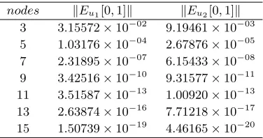
The exact solution is (u1(x), u2(x)) = (ex_{, e}−x_{). Fig. 1 and Table 1 show the} results of applying the interpolation with equally-spaced collocation nodes to make the degenerate approximations for the non-degenerate kernels as well as source functions in Eq. (4.5). In this case, the obtained results are related to the numerical solutions of the corresponding algebraic system. This numerical results are obtained by using the Newton method by increasing the significant digits to 50.

Table 1. Results for Example 4.2.

nodes kEu₁[0,1]k kEu₂[0,1]k

3 3.15572×10−02 ₉_.₁₉₄₆₁_×₁₀−03

5 1.03176×10−04 ₂_.₆₇₈₇₆_×₁₀−05

7 2.31895×10−07 ₆_.₁₅₄₃₃_×₁₀−08

9 3.42516×10−10 ₉_.₃₁₅₇₇_×₁₀−11

11 3.51587×10−13 ₁_.₀₀₉₂₀_×₁₀−13

13 2.63874×10−16 ₇_.₇₁₂₁₈_×₁₀−17

15 1.50739×10−19 ₄_.₄₆₁₆₅_×₁₀−20

(9)

0 1 2 3 4 0

1 2 3 4 5

x u1

H

x

L

0 1 2 3 4

-1.0

-0.5

0.0 0.5 1.0 1.5 2.0 2.5

x u2

H

x

L

Figure 2. _{Comparison of the exact solution with approximation}

solutions given by MDKM for Example 4.3. Solid line: exact solu-tion, dashed line: 9th-order and dotted line: 5th-order approxima-tions.

equa-tions of the second kind with some non-degenerate kernels [13, 8, 9] 

   

u1(x) =x+1₃cos(x) +1₂xsin2(1)−R1

0 tcos(x)u1(t)dt− R1

0 xsin(t)u2(t)dt, u2(x) =f2(x)−R1

0 e xt2

u1(t)dt−R1

0 (x+t)u2(t)dt.

(4.6) wheref2(x) = cos(x) +ex

−1

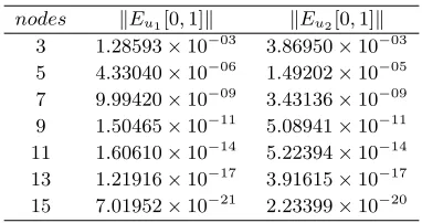
2x + (x+ 1) sin(1) + cos(1)−1. The exact solution is (u1(x), u2(x)) = (x,cos(x)). Fig. 2 and Table 2 show the results of applying the interpolation with equally-spaced collocation nodes to make the degenerate approximations for the non-degenerate kernels as well as source functions in Eq. (4.6). Similar to the Example 4.2, the obtained results are related to the numerical solutions of the corresponding algebraic system. This numerical results are obtained by using the Newton method by increasing the significant digits to 50. It is important to notice that, in Eq. (4.6), we have f2(0) =

1

2+ sin(1) + cos(1).

Table 2. Results for Example 3.

nodes kEu₁[0,1]k kEu₂[0,1]k

3 1.28593×10−03 ₃_.₈₆₉₅₀_×₁₀−03

5 4.33040×10−06 ₁_.₄₉₂₀₂_×₁₀−05

7 9.99420×10−09 ₃_.₄₃₁₃₆_×₁₀−09

9 1.50465×10−11 ₅_.₀₈₉₄₁_×₁₀−11

11 1.60610×10−14 ₅_.₂₂₃₉₄_×₁₀−14

13 1.21916×10−17 ₃_.₉₁₆₁₅_×₁₀−17

15 7.01952×10−21 ₂_.₂₃₃₉₉_×₁₀−20

(10)

5. Conclusion

In this paper, a modified degenerate kernel method (MDKM) was applied to the system of Fredholm integral equations of the second kind. The results show that the MDKM is a promising tool to handle this type of equations. We used the Lagrange polynomials as base functions for needed approxima-tions, and in this case, the MDKM becomes as a collocation method, namely Lagrange-collocation method. The alternative of using Bernstein and Cheby-shev polynomials as well as sinc functions are also possible. Finally, extension of the method to higher dimensional can be accommodated. We pointed out that the corresponding analytical and numerical results are obtained using

Mathematica_.

Acknowledgements

The author would like to thank the anonymous referees for their constructive comments and suggestions. Many thanks are due to the Ilam University of Iran for financial support.

References

1. K. Atkinson,The Numerical Solution of Integral Equations of the Second Kind,

Cam-bridge University Press, UK, 1997.

2. K. Atkinson, W. Han,Theoretical Numerical Analysis (A Functional Analysis

Frame-work), Springer-Verlag, New York, 2009, Third Edition.

3. A. Hashemi Borzabadi, M. Heidari, A Successive Numerical Scheme for Some Classes of

Volterra-Fredholm Integral Equations,Iranian Journal of Mathematical Sciences and

Informatics,10_{, (2015), 1-10.}

4. E. Hetmaniok, D. Slota, T. Trawinski and R. Witula, Usage of the Homotopy Analysis Method for Solving the Nonlinear and Linear Integral Equations of the Second Kind,

Numer. Algor.67_{, (2014), 163-185.}

5. S. Hosseini, S. Shahmorad, F. Talati, A matrix based method for two dimensional

nonlinear Volterra-Fredholm integral equations.Numer. Algor.,68_{, (2015), 511-529.}

6. H. Jafari, M. Alipour, M. Ghorbani, T-Stability Approach to the Homotopy

Perturba-tion Method for Solving Fredholm Integral EquaPerturba-tions,Iranian Journal of Mathematical

Sciences and Informatics,8_{, (2013), 49-58.}

7. K. Maleknejad, M. Shahrezaee, H. Khatami, Numerical solution of integral equations

system of the second kind by Block-Pulse functions,Applied Mathematics and

Compu-tation,166_{, (2005), 15-24.}

8. K. Maleknejad, N. Aghazadeh, M. Rabbani, Numerical solution of second kind

Fred-holm integral equations system by using a Taylor-series expansion method, Applied

Mathematics and Computation,175_{, (2006), 1229-1234.}

9. K. Maleknejad, F. Mirzaee, Numerical solution of linear Fredholm integral equations

system by rationalized Haar functions method,Int. J. Comput. Math.,80_{(11), (2003),}

1397-1405.

10. A. Molabahrami, An algorithm based on the regularization and integral mean value

methods for the Fredholm integral equation of the first kind,Appl. Math. Modelling,

37_{, (2013), 9634-9642.}

(11)

11. A. Molabahrami, Direct computation method for solving a general nonlinear Fred-holm integro-differential equation under the mixed conditions: Degenerate and

non-degenerate kernels,Journal of Computational and Applied Mathematics,282_{, (2015),}

34-43.

12. A. Molabahrami, The relationship of degenerate kernel and projection methods on

Fred-holm integral equations of the second kind,Commun. Numer. Anal.1_{, (2017), 1-6.}

13. J. Rashidinia, M. Zarebnia, Convergence of approximate solution of system of Fredholm

integral equations,J. Math. Anal. Appl.,333_{, (2007), 1216-1227.}

14. A. Shidfar, A. Molabahrami, Solving a system of integral equations by an analytic

method,Math. Comput. Model.,54_{(2011) 828-835.}

15. A. Tari, M. Rahimi, S. Shahmorad, F. Talati, Solving a class of two-dimensional

lin-ear and nonlinlin-ear Volterra integral equations by the differential transform method.J.

Comput. Appl. Math.,228_{, (2009), 70-76.}

16. A.-M. Wazwaz, Linear and Nonlinear Integral Equations: Methods and Applications,

Higher Education Press, Beijin, 2011.