Development of a methodology for collaborative control within a WEC array

Development of a methodology for collaborative

control within a WEC array

Meunier Paul-Emile

, Cl´ement Alain H.

, Gilloteaux Jean-Christophe

, and Kerkeni Sofien

E-mail: [email protected], [email protected], [email protected]

†_{D-ICE Engineering, 1 rue de la Noe, 44300 Nantes, France}

E-mail: [email protected]

Abstract—It has been established that Wave Energy Converters efficiency can be improved by control. One of the main challenges of reactive control is the non-causality of the optimal controller. This study presents a methodology to solve the non-causality issue by providing a deterministic forecast of the controlled body velocities. This forecast is achieved by using the measurements of the states of the most up wave device of the array. The reactive control approach also implies strong instabilities due to the extreme dynamics of the controlled devices. The proposed method suggests to mitigate this behavior by applying a window function on the optimal controller impedance. In order to maximize the efficiency of the resulting control and ensure the robustness of the system, a stability analysis is conducted. Optimal sets of parameters are determined and applied to a time domain simulation of an array of 10 cylindrical floating WECs. The results obtained show an average efficiency of the array of83% of the maximum energy retrievable in the waves.

Index Terms—wave energy converter, optimal control, causal-ity, energy, efficiency, stability

NOMENCLATURE

B(ω) [N.s/m] hydrodynamic damping matrix

Ma(ω) [N.s2/m] added mass matrix

M [kg] mass matrix

Ks [N/m] hydrodynamic stiffness matrix

V(ω), v(t) [m/s] device velocity vector

Fex(ω), fex(t) [N] excitation force vector Fu(ω), fu(t) [N] PTO force vector Ξ(x, ω), η(x, t)[m] surface elevation

Zi [N.s/m] intrinsic impedance matrix

Znet [N.s/m] net impedance matrix

Zu [N.s/m] controller impedance matrix

hu,m,n [N.s/m] controller impulse response

tprev [s] forecast time

f [Hz] frequency

Hs [m] significant wave height

Tp [s] peak period

I. INTRODUCTION

Wave Energy Converters (WEC) are devices able to retrieve a part of the energy contained in the waves and to convert it into electricity. These systems are excited by wave energy which is then absorbed by a sub-system called the Power Take-Off (PTO). Many studies have been performed to increase the efficiency of the WECs and therefore improve the bankability of wave energy in the very competitive market of energy.

These efficiency improvements are performed using a suitable real-time control. In order to retrieve a maximum of energy, in regular waves the machines should be in resonance with the waves. More specifically the velocity of the floating body should be in phase with the excitation force of the incoming wave. A first step toward this goal is to dimension the floating body to tune its natural frequency to the one of the dominant sea state observed at the installation area. Nevertheless, in irregular waves the system will never be in resonance with each of the components of the spectrum. Some sophisticated control strategies such as the latching [1] tend to improve this behavior by adapting the system wave by wave but still using a passive PTO. Now, considering a reactive PTO which is bidirectional, i.e. for which it is possible to retrieve and give energy to the system, many types of control can achieve an even better efficiency, as for instance the Model Predictive Control (MPC) [8]. The common thread between these reactive PTO control strategies is to instantly adapt the natural frequency of the system to the instantaneous frequency of the incident wave.

The impedance of the optimal controller is well known and can easily be derived in frequency domain. However, to actually perform this control in the real physical world, it has to be implemented in time domain. This implementation is by far not as trivial as the frequency form. The impulse response of the optimal controller is non causal [6] [10], which implies that the excitation force on the body has to be known, then predicted, over a near future. This forecast can be performed, for instance, by using wave gauges and using a wave propagation model. However it would involve a high installation and maintenance costs. Moreover, a large number of gauges must be in place to surround the farm and adapt to the wave direction modifications. In this work, the information necessary to control one or several WECs is proposed to be deduced from the dynamics of the other bodies in an array. More precisely, the velocity of an up-wave body is used to forecast the velocity of a down-wave device. This makes possible the application of optimal control.

Optimal control on a WEC produces an extremely intense dynamic of the system. The amplitude of the device can easily reach 5 times the amplitude of the incoming waves. Theoret-ically, the amplitude and velocity tend to infinity when the

SPECIAL ISSUE OF THE TWELFTH EUROPEAN WAVE AND TIDAL ENERGY CONFERENCE, 27 SEPTEMBER - 1 AUGUST 2017, CORK, IRELAND

©EWTEC 2017. THIS IS AN OPEN ACCESS ARTICLE DISTRIBUTED UNDER THE TERMS OF THE CREATIVE COMMONS ATTRIBUTION 4.0 LICENCE (CC BY

h p://creativecommons.org/licenses/by/4.0/). UNRESTRICTED USE (INCLUDING COMMERCIAL), DISTRIBUTION AND REPRODUCTION IS PERMITTED PROVIDED THAT CREDIT IS GIVEN TO THE ORIGINAL AUTHOR(S) OF THE WORK, INCLUDING A URI OR HYPERLINK TO THE WORK, THIS PUBLIC LICENSE AND A COPYRIGHT NOTICE.

wave frequency tends to zero or infinity. Even for frequencies close to the natural frequency of the device, the amplitude can be really higher than the wave and increases when the wave frequency move off. This behavior of the optimal control brings many design and modeling issues: the small amplitude hypothesis used in linear theory is no longer respected, the controller is unstable, and the ratio between total and net power is huge which implies no energy yield if the efficiency of electric chain is included in the model [9]. To cope with these issues, a window is applied on the controller impedance to ensure the stability of the system in the area of interest.

II. METHODOLOGY OF THE CONTROLLER

A. Framework of the study

Within the framework of this study, generic point absorbers oscillating in heave only are considered. The WEC array is composed of identical floating cylinders that have the following characteristics:

• radius5m

• draft10m

• mass8.05_·105_kg

• water depth 50m

This example is chosen in order to get high accuracy analytical results of the hydrodynamic coefficients using the method developed in [5]. This allows to get a good a consistency between the coefficients even for the high frequencies (over the frequencies where the Response Amplitude Operator tends to zero) which is important in a didactic point of view to explain the behavior of velocity transfer functions (II-E). However, this level of accuracy is not needed for the proper working of the method as the dynamic of the floating bodies never reaches these frequencies. Moreover, different body geometries can be considered using ad-hoc softwares such as the open-source solution NEMOH [2], developed at LHEEA lab, to compute the hydrodynamic coefficients.

B. Theoretical background

The hydrodynamic coefficients are obtained using potential linear theory in frequency domain. For the sake of clarity, only one degree of freedom (heave) is considered for each body. Then, in frequency domain, the equation obtained from the fundamental principle of dynamic for aN body array can be expressed as

B(ω) +jω[M+Ma(ω)−

Ks

ω2]

V(ω) =Fex(ω)+Fu(ω)

(1) whereB(ω)andMa(ω)are respectively the hydrodynamic

damping and added mass[N, N]sized matrices. The diagonal terms correspond to the direct terms i.e. the force of the body on itself, and the extra diagonal terms correspond to the crossed terms i.e. the forces applied from a body to another one. M and Ks are respectively the mass and hydrostatic

stiffness [N, N] sized diagonal matrices. V(ω),Fex(ω), and

Fu(ω)are respectively the velocity, excitation force, and PTO

force[N]sized vectors.

The parameters B(ω),Ma(ω),M andKsdepends on the

geometry of the floating body and govern its dynamics. It is convenient to gather these terms in a compact formZiwhich

represents the intrinsic impedance of the system, as below

Zi=B(ω) +jω[M+Ma(ω)−

Ks

ω2] (2)

which gives the compact form of the dynamic equation

ZiV(ω) =Fex(ω) +Fu(ω) (3)

The second member of equation 3 contains the forces applied to the system. The excitation force Fex(ω) =

Hex(ω)Ξ(x, ω), where Hex(ω) is the excitation force

coef-ficient [N] sized vector and the scalar Ξ(x, ω) is the Fourier transform of the free surface elevation at the reference point of the domain, account for the effects of the potentials of the incident and diffracted wave on the system. The PTO force

Fu(ω)is the force applied to the system in order to extract or

supply energy to the system.

To get the equation of motion in time domain, an inverse Fourier transform is applied to equation 3. The result for one body is the so called Cummins equation [4].

[M+Ma∞] ˙v(t) +

ˆt

−∞

h(t−τ)v(τ)dτ+Ksx(t) =fex(t) +fu(t) (4)

In the case of a WEC array, a system of linear equations is formed instead of a scalar for equation 4. The convolution kernelh(t)represents the radiation force and is defined as the following inverse Fourier transform:

h(t) =_F−1_{B(ω) +jω[Ma(ω)−Ma∞]} (5) C. Optimal control

The control of the WEC is achieved by applying a force on the system using the PTO. By doing so, the dynamic of the system is modified, so that the performances of the device are improved. The impedance of the optimal controller is well known and is easily shown to be the conjugate of the intrinsic impedance of the system [7], which gives the following formulation of the PTO force:

Fu(ω) =−Z¯i(ω)V(ω) (6)

As the impedance of the system is a complex number, the controller is alternatively supplying energy to the system and then taking it back. When the energy flux is oriented to the system, the power is considered reactive. This energy given to the system is not lost as it generates a global improvement on the total energy recovered. Though, the losses associated to the efficiency of the PTO are always present whatever the energy flux orientation and are consequently cumulating. Practically, there are energy losses when supplying energy to the system and when recovering the energy which can drastically reduce the efficiency of the whole system [9]. The term Fu(ω)

impedances can be factorized which allows to obtain the net impedance of the system:

Zi(ω) + ¯Zi(ω)V˜(ω) =Fex(ω) (7)

2_<[Zi(ω)]V˜(ω) =Fex(ω) (8)

Znet(ω)V˜(ω) =Fex(ω) (9)

Equation 9 gives two conditions on the behavior of the controller. As the net impedance is purely real, the velocity of the bodies are synchronized with the excitation force applied on them (the phase condition) and the amplitude of the controller is defined as V(ω) = Fex(ω)/2B(ω) (the

amplitude condition). Most of control strategies are based on phase control but optimal reactive control is more specifically putting the system in a permanent resonance state by adapting the system natural frequency to the incident wave to wave period.

D. Non causality of the controller

As the control of the WEC is performed in real time, the expression of the controller transfer function has also to be defined in time domain. The instantaneous force applied to the PTO is obtained by an inverse Fourier transform of equation 10:    Fu,I .. . Fu,N   =−    ¯

Zi,I,I · · · Z¯i,I,N

..

. . .. ... ¯

Zi,N,I · · · Z¯i,N,N

      VI .. . VN    (10)

⇓ F−1

      

fu,I(t) =P N n=I

´+∞

−∞ hu,I,n(t−τ)vn(τ)dτ

.. .

fu,N(t) =P N n=I

´+∞

−∞ hu,N,n(t−τ)vn(τ)dτ

(11)

withhu,m,n(t) =

´+∞

−∞ Z¯i,m,n(ω)e

+iωt_dω

wheren is referencing to the body generating the force, and mto the body affected by it.

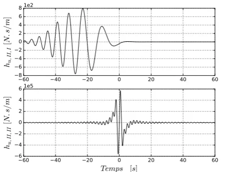
When doing this operation, one of the challenges of optimal control appears. The impulse responses hu,m,n(t) of optimal

controller prove to be non causal (Figure 1 on page 3) which is revealed by a non null impulse response in the negative times. A non causal impulse response corresponds to a response of the system preceding the input. Practically, the only way to compute the convolutions and therefore the optimal force to apply to the PTO, in order to get a maximal absorption of the energy contained in the wave, would be to forecast the velocities of the controlled devices.

However, it’s worth noting that magnitude of the impulse response of the off-diagonal term is significantly inferior to the one of the diagonal term and therefore can be neglected.

60 40 20 0 20 40 60

8 6 4 2 0 2 4 6 8

h

,I

[

N

.s

/m

]

60 40 20 0 20 40 60

Temps

[

s

]

h

[

N

.s

/m

]

Fig. 1. Impulse responses of controller impedances for the down-wave device of a two body array spaced by 200m. The kernel hu,II,I (up) corresponds to the crossed term and the kernelhu,II,II(down) corresponds to the direct term.

This is an interesting property as taking into account the off-diagonal term would imply a way longer forecast horizon to cancel the non causality. The farm geometry condition that could allow to include the crossed terms of the controller is a pattern where the controlled devices are close together (to ensure short radiation impulse responses) and the distance to the first up-wave device is sufficiently large to ensure a long enough forecast horizon.

In brief, in order to compute the PTO force, the forecast of the controlled body velocity is essential. The collaborative control strategy aims at providing the velocity forecast for the control bodies by gathering this information from the state vector of the most up-wave body in the array.

E. Velocity forecast from neighbor velocity

The velocity forecast is made possible by establishing the transfer functions connecting the device velocity of the different floating bodies composing the array. The input of the system is defined as the velocity of the most up-wave device with respect to the wave direction, and the output is the velocity of the down-wave devices. From the equation of motion in frequency domain (3), it as achievable to deduce this relation.



  

Znet,I,I · · · Znet,I,N . . . . .. . . .

Znet,N,I · · · Znet,N,N         VI . . . VN     =     Hex,I . . . Hex,N     Ξ (12)



   

Hex,I Znet,I,II · · · Znet,I,N .

. .

. .

. . ..

. . .

Hex,N Znet,N,II · · · Znet,N,N 

    

   

Ξ

VII . . .

VN 

   

=



   

Znet,I,I . . .

Znet,N,I 

   

VI (13)

Written in a more compact form as:

ZMVM =ZIVI (14)

The solution of this linear system for each frequency gives the free surface elevation and the velocity of the floating bodies of the array, as a function of the velocity of the up-wave body (15):

Hv(ω) =Z−_M1(ω)ZI(ω) (15)

The Hv matrix obtained, contains the transfer function

Ξ/VI linking the free surface elevation to the velocity of the

up-wave body, and the transfer function Vn/VI linking the

velocities of the down-wave devices to the up-wave one. From now on, the Hv matrix will be called the velocity transfer

function.

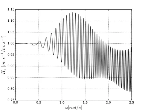
In the case of an array composed of two devices spaced by a distance of200m, the velocity transfer function is presented in Figure 2 on page 4. For low frequencies, the function tends toward 1 as the wavelengths tend toward infinity so the two floating bodies are synchronized. As the frequency increases the function starts to oscillate, so each body will alternatively benefit from the group effect of the array as a function of the wavelength. The behavior of the transfer function in high frequencies does not present any major interest as the RAO of the bodies is null in this frequency band, so there is no displacement.

0.0 0.5 1.0 1.5 2.0 2.5

ω

[

rad/s

]

0.80 0.85 0.90 0.95 1.00 1.05 1.10 1.15

H

[

m

.s

−

1

/m

.s

−

1

]

Fig. 2. Amplitude of the velocity transfer functionHv, linking the velocity of the up-wave device to the one of the down-wave device in the case of an array composed of two devices spaced by200m.

With the aim of getting the temporal response of this trans-fer function, an inverse Fourier transform should be applied to

it and the result should be convoluted with the velocity of the up-wave device. This allows to get the optimal velocity of any floating body in the array in real time, however the values are obtained at the present time and does not constitute a forecast of the velocity.

F. Pseudo-causal form of the controller

The forecast of the velocity is obtained by taking advantage of the propagation time of the waves between the up-wave device and the down-wave device. This propagation time is exposed in the impulse response of the velocity transfer function with a visible delay increasing as the distance with the up-wave device increases. For the calculation, in time domain, of the velocity of the down-wave devices, it is possible to apply a change of variable in the convolution kernel in order to obtain the velocity values at the different time (17), which corresponds to a time shift of the convolution kernel. Yet, this is possible as long as the velocity transfer function impulse response stays causal, which implies to stay in the limit of the forecast horizon. The value of this time shift is, in a first approach, chosen as the limit value of the forecast horizon tprev.

vn(t) =

ˆ +∞

−∞

hv,n(t−τ)vI(τ)dτ (16)

vn(t+tprev) =

ˆ +∞

−∞

hv,n(t+tprev−τ)vI(τ)dτ (17)

The time shift of the impulse response of the velocity transfer function has allowed to obtain the velocity forecast needed to perform the calculation of the force to apply to the PTO in order to get the maximum efficiency of the optimal reactive control. It is important to notice that the first up-wave body cannot be optimally controlled as there is no up-wave body to provide it the velocity forecast. The optimal control force is equal to the sum of the convolution of the direct impedance term with the controlled body velocity and the convolutions of the non diagonal terms with the velocities of the other bodies. This corresponds to apply the control corresponding to the dynamics of the body itself and taking into account the radiation forces from the other bodies. As mentioned previously (II-D), the contribution of the non diagonal terms of the controller impedance are here considered as negligible. Consequently, only the direct term is retained in the calculations (18).



  

  

fu,II(t) =

´+∞

−∞ hu,II,II(t−τ)vI(τ)dτ

.. .

fu,N(t) =

´+∞

−∞ hu,N,N(t−τ)vI(τ)dτ

(18)

With the forecast obtained previously, the velocities of the controlled bodies can be expressed asvn(τ+tprev). In order



  

  

fu,II(t) =

´+∞

−∞ hu,II,II(t−tprev−τ)vI(τ+tprev)dτ

.. .

fu,N(t) =

´+∞

−∞ hu,N,N(t−tprev−τ)vI(τ+tprev)dτ

(19) The new impulse responses of the controller are conse-quently shifted to the right. If the controlled bodies are sufficiently distant from the up-wave body, then the impulse response becomes pseudo-causal (Figure 3 on page 5), i.e. the impulse response in the negative time is almost null. Consequently, it is possible to compute the force to apply to the PTO in a deterministic way, with a low error.

30 20 10 0 10 20 30 40

Temps

[

s

]

4 2 0 2 4 6

h

II

,I

I

[

N

.s

/m

]

1e5

hu hu+tprev

Fig. 3. Time shift of the controller impulse responsefor the down-wave device of an array composed of two bodies spaced by200m.

To sum up the modifications applied to the controller impedance, the non diagonal terms are set to zero, and the first up-wave body is set to have a passive PTO as it cannot be controlled by applying the current method. These modi-fications leads to the new form of the controller impedance (20):

Zu=



    

BP T O 0 · · · 0

0 Z¯i,II,II . .. ...

..

. . .. . .. 0

0 _{· · ·} 0 Z¯i,N,N



    

(20)

The control strategy suggests to use the up-wave body, with respect to the wave orientation, as a sensor in order to provide velocity forecasts for the rest of the array which allows to apply a reactive control on it. Though the first body cannot be controlled in the same manner, a passive PTO can still be applied on it which increases the overall efficiency of the array. The first up-wave body is consequently not only a sensor but a productive element of the WEC array. Moreover, as the direction of the waves may vary over time, the up-wave body can be a different device over time. This eases significantly the

adaptability of the forecast with respect to the wave orientation variations without the need of installing specific sensors all around the farm.

III. CONTROLLER INSTABILITIES AND WINDOWING

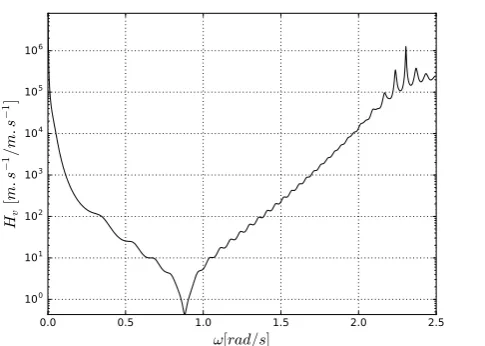
The collaborative control strategy has empowered the reac-tive control strategy on a WEC array. Yet, another challenge appears when dealing with optimal reactive control. The amplitude, and velocity of a floating body subject to optimal reactive control tend to infinity when frequency tends to zero and infinity, and present a minimum at the natural frequency of the system. These characteristics of the optimal reactive control implies extreme forces to apply to the PTO which induces instability to the controller. As the first up-wave body is controlled with a passive PTO, its motion will be maximal at its natural frequency and decreases around this point. The large difference in the dynamics of the controlled bodies and the up-wave body leads to a major change in the velocity transfer function (Figure 4 on page 5).

0.0 0.5 1.0 1.5 2.0 2.5

ω

[

rad/s

]

101 102 103 104 105 106

H

[

m

.s

−

1

/m

.s

−

1

]

Fig. 4. Amplitude of the velocity transfer function in logarithmic scale in the case of the up-wave body controlled with a passive PTO, for the down-wave device of an array composed of two bodies spaced by200m.

of the RAO and the bandwidth of the wave spectrum. The RAO gives the high frequency cut from which the body is not moving anymore, and the wave spectrum gives the low frequency cut with the highest wavelength found in it. When the window is applied, the controller is sub optimal, but its behavior stays close to optimality in the operational domain of the machine. These criteria present a good first approach to calibrate the controller window but the parameters can be tuned finely using a sensibility analysis methodology.

Furthermore, to limit the extreme behavior of the optimal control when the peak frequency of the sea state gets far from the natural frequency of the machine, the WEC should be designed to be naturally tuned with the dominant sea state where the machine is supposed to be set up. Also, the machine could be adapted to the slow variations of the sea states by varying the stiffness of a PTO added to the controller or by varying the mass of the machine using, for instance, ballast water management.

IV. SENSIBILITY ANALYSIS

This part of the study aims to provide a methodology whose purpose is to define the domain of stability of the controller, the best parameters, and the maximum energy retrievable by the farm.

A. Domain of the study

The domain of the study is established by defining the studied response and the factors that may have an effect on it and eventually the levels (values) of these factors used in the simulations. Here the studied response of the system is the energy harvested by the devices in order to maximize the overall efficiency of the farm. More precisely, an optimality coefficient (defined in IV-B) will be defined to refer to a normalized approach of the energy retrieved. It is important to notice that the selection of this response seems trivial but some other responses may be of interest when dealing with optimal reactive control such as the ratio between the total exchanged power and the net power retrieved. This point will be more extensively detailed in a future work. Concerning the factors, the bandwidth of the controller window has been shown to have an impact on the stability of the system and the energy retrieved which places it as a good candidate for the study. Likewise, the bandwidth of the controller window should be adapted to the peak period of the wave, so the impact of this factor is also of fundamental importance. Another essential factor is the forecast time. As seen in II-F, if the forecast time is too small the controller impulse response cannot be efficiently causalized and if the forecast time is too large, the velocity transfer function impulse response becomes non causal. Lastly, the forecast time is obviously related to the distance between the controlled body and the first up-wave body. The levels of the factors, i.e. the different values of the factors at which the output is evaluated, are chosen from previous expertise to limit the number of calculations while ensuring a sufficient range and resolution of the response (Table I on page 6).

Factor Levels

Distance [m] 200,400,600

Forecast time [s] 8,10,12,15,20,30

Peak period [s] 6,9,12

Low frequency cut [rad/s] 0.2,0.35,0.5,0.65,0.8

High frequency cut [rad/s] 1.0,1.5,2.0,2.5,3.0,3.5

TABLE I

FACTOR LEVELS EVALUATED IN THE STUDYANALYSIS IN THE CASE OF

AN ARRAY COMPOSED OF TWO BODIES SPACED BY200m.

Regarding the fixed parameters, an array of two WECs is chosen for this study. The simulations are run over a physical time of 30 minutes with a time step of0.05s. Each simulation is performed 10 times with a different phase set chosen randomly, then the response is averaged. The numerical integrations are performed with a Runge-Kutta 4 integrator. The significant wave height of the sea state is equal to2mbut this has no impact on the response as the model is fully linear. Also, the wave spectrum model used for the simulations is a Bretschneider spectrum defined by equation (21) [3].

S(f) = 5 16H

2

sfm4f−5e

[−5

4(

f fm)

−4_]

(21)

B. Optimality coefficient

The analysis of the energy retrieved by a WEC is not straightforward as the power contained in the wave varies with the peak period of the sea state and the maximal theoretical power of device may vary due to the farm effects. In order to ease this analysis, an optimality coefficient is defined as the ratio between the mean power actually retrieved Pmean,

over the theoretical maximumPth(26). First, the velocity and

the PTO force are calculated including the wave spectrum amplitude (22, 23), then the power absorbed vector PA(ω)

(24) is calculated taking into account the farm effects and using the full optimal control impedance for Zu. Lastly, the

maximum theoretical power is obtained by doing the sum of

PA(ω)over the frequencies (25).

V(ω) = [Zi(ω) +Zu(ω)]−1a(ω)Hex(ω) (22)

Fu(ω) =−Zu(ω)V(ω) (23)

PA(ω) =−

1 2<

F ¯V (24)

Pth=

X

PA(ω) (25)

Copt= 100

Pmean

Pth

(26)

C. Response analysis

Concerning the impact of the distance separating the con-trolled device to the up-wave body, the optimal forecast time increases with the distance. This observation was expected as the waves take a longer time to propagate from the sensor device to the controlled one. Therefore, a longer forecast time can be used without stepping in the non causal alteration of the velocity transfer function impulse response. With a longer time, the non causal part of the controller impulse response is even more reduced which produces a better efficiency.

The optimal value of the low cut-off frequency is mainly driven by the peak period of the sea state and the distance between bodies. The controller window size has to be set according to the wave spectrum in order to ensure a maximum efficiency. Thus, when the period of the wave increases, the controller window low cut-off frequency has to decrease to fit with the repartition of the energy. The distance impacts this parameter because a longer distance implies a longer forecast time. Waves with large wavelengths propagate faster, therefore longer wave periods can be causalized with a longer forecast time, hence the energy of the corresponding waves can be retrieved more efficiently.

The variation of the optimal value of the high cut frequency is slightly more subtle. In a general way, the high cut frequency optimal value is decreased as the peak period increases for the same reasons that the low cut frequencies vary. However, in some circumstances, two local maxima can appear. A local maximum operating with a widely opened window centered over the wave spectrum and another local maximum with a narrower window.

Peak period of 6s

Distance [m] 200 400 600

Forecast time [s] 10 15 20

Low cut frequency [rad/s] 0.5 0.5 0.5 High cut frequency [rad/s] 3.5 3.5 3.5

Peak period of 9s

Distance [m] 200 400 600

Forecast time [s] 10 15 20

Low cut frequency [rad/s] 0.35 0.35 0.2 High cut frequency [rad/s] 2.0 1.5 3.0

Peak period of 12s

Distance [m] 200 400 600

Forecast time [s] 10 15 20

Low cut frequency [rad/s] 0.2 0.2 0.2 High cut frequency [rad/s] 2.5 1.5 1.5

TABLE II

OPTIMAL PARAMETERSIN THE CASE OF AN ARRAY COMPOSED OF TWO BODIES

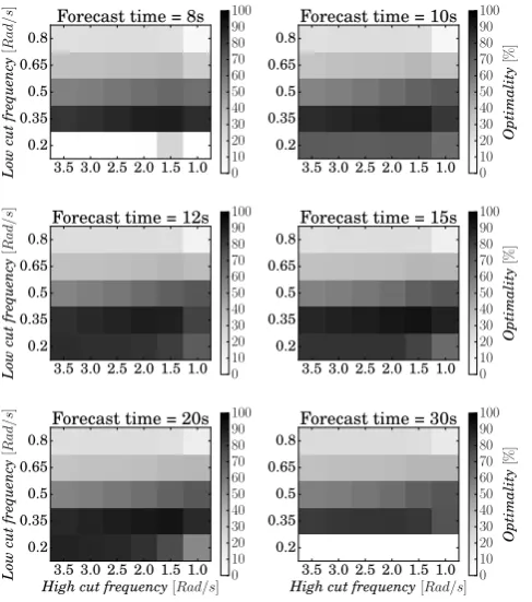
The study of the stability as a function of the different factors is another important part of the study. In order to portray the behavior of the system, one can fix the external factors and then visualize the optimality coefficient matrices as a function of the internal parameters (Figure 5 on page 7). Here, the bottom left corner of each matrix represents the narrowest window and the top right corner, the widest window of the controller impedance. In some cases the simulations have shown that the controller became instable. In these

situations the average power obtained tends to _−∞ so the results are arbitrarily set to zero percent of optimality for clarity sake.

In the cases where the appropriate forecast time is selected, the stability area is sizable and the first instable points of operation are far away from the optimal operational point. Moreover, the gradient around the maximum point is quite low which provides more than 50% of optimality in a large range of internal parameters. Concretely, this ensure some robustness of the system to external changes. However, when the forecast time is to short or to large, instable operational points can appear close to the maximum points. In these cases, the stability of the system cannot be assured. This shows the importance of the stability analysis when deploying a reactive control strategy. Also this behavior can be explained by the fact that the maximum efficiency point is obtained when the low frequency cut is at a low level. In these conditions the window is large and tends to retrieve the whole energy of the wave spectrum, however increasing a little bit this window adds waves that cannot be causalized.

The forecast time has a big range of acceptable values which increases with the distance between bodies. As soon as the time is long enough to causalize the controller impulse response without un-causalize the velocity transfer function impulse response, the optimality coefficient matrix is virtually not impacted by the forecast time. This behavior consolidates the robustness of the system.

1.0 1.5 2.0 2.5 3.0 3.5 0.2 0.35 0.5 0.65 0.8 Low cut frequency [ R ad/s ]

Forecast time = 8s

0 10 20 30 40 50 60 70 80 90 100 1.0 1.5 2.0 2.5 3.0 3.5 0.2 0.35 0.5 0.65 0.8

Forecast time = 10s

0 10 20 30 40 50 60 70 80 90 100 Optimality [%] 1.0 1.5 2.0 2.5 3.0 3.5 0.2 0.35 0.5 0.65 0.8 Low cut frequency [ R ad/s ]

Forecast time = 12s

0 10 20 30 40 50 60 70 80 90 100 1.0 1.5 2.0 2.5 3.0 3.5 0.2 0.35 0.5 0.65 0.8

Forecast time = 15s

0 10 20 30 40 50 60 70 80 90 100 Optimality [%] 1.0 1.5 2.0 2.5 3.0 3.5

High cut frequency[Rad/s]

0.2 0.35 0.5 0.65 0.8 Low cut frequency [ R ad/s ]

Forecast time = 20s

0 10 20 30 40 50 60 70 80 90 100 1.0 1.5 2.0 2.5 3.0 3.5

High cut frequency[Rad/s]

0.2 0.35 0.5 0.65 0.8

Forecast time = 30s

0 10 20 30 40 50 60 70 80 90 100 Optimality [%]

V. SIMULATION OF A10BODY ARRAY

The stability analysis of the previous section has allowed to determine the optimal parameters to apply to the controller in order to maximize its efficiency. These parameters are herein tested on a 10 body farm configuration. The geometry of the farm is presented in Figure 7 on page 8, the controlled bodies are positioned in a square pattern and every devices is spaced of200m. The waves propagates from the left to the right and the first upwave body is equipped with a passive PTO tuned to the sea state conditions. The purposes of this simulation are to show that the results obtained for a two body array can be extended with a good efficiency to an array composed of more devices and that the collaborative control methodology is effective in these conditions.

The simulation is run over a physical time of 60 minutes with a time step of0.01sin sea state conditions ofHs= 2m

significant wave height and Tp = 9s peak wave period with

a Bretschneider spectrum (21). The numerical integrations are performed with a Runge-Kutta 4 integrator.

A. Velocity forecast

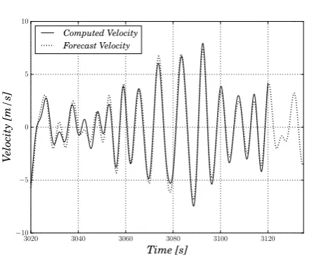
The velocity forecast is one of the key element of the method and should be the first result to check in order to make sure that the control can be performed in suitable conditions. In the case of the farm geometry studied here, the more significant velocity forecast is the one of the central body. This device is the most affected by the radiation forces of all the other devices especially due to the reactive control applied on them which induces important velocities and therefore con-siderable radiation forces. The forecast velocity is compared to the actual velocity computed during the simulation (Figure 6 on page 8).

3020 3040 3060 3080 3100 3120

Time [s] −10

−5 0 5 10

Velocity

[m/s]

Computed Velocity Forecast Velocity

Fig. 6. Comparison between the forecast velocity and the computed velocityof the central body of a 10 body array.

On the whole, the forecast velocity fits very well the actual velocity of the device but it is important to note that the forecast is more accurate on the long period waves than on the short period ones. On the short period waves where

the direction of the device velocity changes many times in few seconds, the forecast can be quite inaccurate, which will produce a poor control on this short amount of time. However these waves represent a small part of the whole energy contained in the spectrum which eventually induces a minimal efficiency drop.

B. Energy distribution

The maximum power retrievable by the machines taking into account the farm effects is calculated in the frequency domain in the same manner as in section IV-B. The results are presented in the case of a fully optimal controller impedance Zu = ¯Zi and for the modified controller impedance with

the off diagonal terms removed and the window applied on it (Figure 7 on page 8).

The first observation is that the passive PTO has a signifi-cantly smaller power capability than the reactive control with about a 8 time ratio. Also, in the first scenario, the farm effects are really important as the less energetic controlled device has a power capability of109kW and the most energetic one 468kW. As a reminder, all the WECs of the array are identical. In the case of the modified controller impedance, the variation of power between the devices of the array is less important with a minimum of 228kW and a maximum of 307kW. Moreover, there is a complete redistribution of the energy between the two scenarios where the less energetic body in the first case becomes the most energetic one. Therefore, the optimality coefficient used in the time domain simulation must be calculated using the modified controller theoretical power. However, the average power of the farm obtained in time domain should be compared to the average theoretical power of the farm with the fully optimal controller.

Concerning the average power, in the scenario of the fully optimal controller, the average theoretical power reaches 284kW, including the first up-wave body equipped with a passive PTO. In the second scenario, it reaches242kW which represents an efficiency drop of 15%. Nevertheless that’s the price you pay to ensure the stability and the causality of the system.

0 100 200 300 400 500 600

Position[m]

−200

−100 0 100 200

Posit

ion

[

m

]

36 342 350

350 468

109

468 190 336 190

0 100 200 300 400 500 600

Position[m]

−200

−100 0 100 200

Posit

ion

[

m

]

36 281 277

277 265

307

265 228 258 228

C. Optimality results

Due to optimal parameters obtained in the sensibility anal-ysis performed in section Section IV, the results produced with the time domain simulation show an excellent energetic production with the collaborative control strategy (Figure 8 on page 9). This confirms that the stability analysis on 2 bodies was a sufficient approximation for the 10 body array and that the collaborative control strategy can efficiently solve the non causality issue of the optimal reactive control, providing a deterministic velocity forecast of the controlled devices.

The results obtained in time domain are in good accordance with maximum theoretical power foreseen with the modified windowed controller with differences between1%and6%but always inferior to the maximum theoretical. All the controlled bodies present an optimality coefficient above 94%. The average power of the farm calculated in time domain is235kW which represents an efficiency drop of 3% compared to the modified windowed controller, which can be attributed to the pseudo causal approximation of the controller.

Lastly, the average power obtained in time domain reaches 83%of the maximum theoretical power retrievable with a fully optimal reactive control.

0 100 200 300 400 500 600

Position[m]

−200

−100 0 100 200

Posit

ion

[

m

]

35 272 267

267 263

303

263 218 244 218

0 100 200 300 400 500 600

Position[m]

−200

−100 0 100 200

Posit

ion

[

m

]

BPTO 97% 97%

97% 99%

99%

99% 96% 94%

96%

Fig. 8. Mean powers(left)and optimality coefficients(right)obtained in time domainfor a 10 body farm configuration. The first upwave body at the position [0, 0] is equipped with a passive PTO and all the others are operated with the collaborative control strategy.

VI. CONCLUSION

This study has shown the possibility to use the information from the up wave devices of the farm in order to solve the non causality of the optimal controller. To do so, the collabo-rative control strategy provides a deterministic forecast of the controlled body velocities using the velocity measurements of the up wave device of the array. Doing so, it is possible to get a pseudo-causal form of the controller. The non stability of the optimal reactive controller has also been highlighted. This challenge of the reactive control is solved by applying a window on the controller impedance.

In order to minimize the impact of the windowing on the control efficiency and to ensure the robustness of the controller, a stability analysis methodology has been developed and conducted. Optimal parameters of the method have been found for different sea state conditions and farm config-urations. The domain of stability has also been assessed, ensuring the robustness on a considerably large operational domain. Moreover, links between the different factors have

been highlighted thus helping to understand the behavior of the controller.

Lastly, a simulation of an array of 10 bodies have been car-ried out using the collaborative control strategy. The stability analysis performed on two bodies has proven to be a good approximation for the 10 body array. As a matter of facts, the time domain results obtained have shown an average 97% optimality coefficient compared to the maximum theoretical power of the modified windowed controller. Comparing to the fully optimal controller, which corresponds to the theoreti-cal maximum energy retrievable form the waves, the results presents 83%of efficiency.

It is important to remind that the method relies on a fully linear theory. The dynamics of the WECs obtained here does not respect the small amplitude hypothesis of the fully linear approach, which implies that the results may not be accurate and should be mitigated. Moreover, the high dynamics of the system implies considerable forces to apply to the PTO that would imply a really powerful machinery. These challenges could be sorted out with the stability analysis methodology by choosing another response to optimize. This response could take into account force and amplitude limitations as well as a constraint on the energy supplied to the device. This approach will be presented in a future work.

REFERENCES

[1] Aur´elien Babarit and Alain H. Cl´ement. Optimal latching control of a wave energy device in regular and irregular waves. Applied Ocean Research, 28(2):77–91, 2006.

[2] Aur´elien Babarit and G´erard Delhommeau. Theoretical and numerical aspects of the open source BEM solver NEMOH. In11th European Wave and Tidal Energy Conference (EWTEC2015), 2015.

[3] Charles L Bretschneider. Hurricane design-Wave practices.Transactions of the American Society of Civil Engineers, 124(1):39–62, 1959. [4] W E Cummins. The impulse response function and ship motions.

Technical report, 1962.

[5] Francesc Fabregas Flavia. A numerical tool for the frequency domain simulation of large clusters of wave energy converters. PhD thesis, Centrale Nantes, 2017.

[6] Johannes Falnes. On non-causal impulse response functions related to propagating water waves. Applied Ocean Research, 17(6):379–389, 1995.

[7] Johannes Falnes. Ocean waves and oscillating systems: linear inter-actions including wave-energy extraction. Cambridge university press, 2002.

[8] Francesco Fusco and John Ringwood. A study on Short-Term Wave Forecasting for time-domain Control of Wave Energy Converters.IEEE Transactions on Sustainable Energy, 1(2):99–106, 2010.

[9] Romain Genest, F´elicien Bonnefoy, Alain H Cl´ement, and Aur´elien Babarit. Effect of non-ideal power take-off on the energy absorption of a reactively controlled one degree of freedom wave energy converter.

Physics Procedia, 48:236–243, 2014.