Int. J. IndustrialMathematics (ISSN 2008-5621)
Vol. 12, No. 1, 2020 Article ID IJIM-1075, 9 pages Research Article
Computing the Matrix Geometric Mean of Two HPD Matrices: A
Stable Iterative Method
F. Kiyoumarsi∗†
Received Date: 2017-05-13 Revised Date: 2018-05-18 Accepted Date: 2019-06-18
————————————————————————————————–
Abstract
In this paper, a new iteration scheme for computing the sign of a matrix which has no pure imaginary eigenvalues is presented. Then, by applying a well-known identity in matrix functions theory, an algorithm for computing the geometric mean of two Hermitian positive definite matrices is constructed. Moreover, another efficient algorithm for this purpose is derived free from the computation of principal matrix square root. Finally, some tests are given to show their applicabilities.
Keywords: Iterative methods; HPD; Sign function; Stability; Convergence.
—————————————————————————————————–
1
Introduction
F
utentions of many researchers in Mathematicsnctions of matrices have attracted the at-due to several applications, refer to [9, pages 26-29] or [4,5,6]. Here, we focus on the computation of the geometric mean of two complex Hermitian positive definite (HPD) matrices, [10].For two HPD matrices, the mean GM(M, N) can be expressed uniquely as [17]
GM(M, N) =M#N :=M(M−1N)12. (1.1)
This is a special form of the more general map:
M#tB :=M(M−1N)t, t∈R, (1.2)
which has a geometrical interpretation as the parametrization of the geodesic joining M and
∗Corresponding author. kumarci [email protected], Tel:+98(913)1819862.
†Department of Mathematics, Shahrekord Branch, Is-lamic Azad University, Shahrekord, Iran.
N for a certain Riemannian geometry onPn, i.e., the set of n×n HPD matrices, [15].
It can be proved that M#N verifies all the properties required by a geometric mean [10], like
M#N =N#M, (1.3)
and ifM andN commute, thenM#N = (AB)12.
Thus, the definition is well established.
Notice that M#N solves the equation of Ric-cati:
Y M−1Y =N, (1.4)
and it can be proved that it is the unique posi-tive solution [2, page 106]. Moreover, using the properties of the principal square root one can derive
M#N =M(M−1N)12 = (N M−1) 1 2M =
N(N M−1)12 = (M N−1) 1
2N. (1.5)
Here we refer to Y as the principal matrix square root of M and write Y = M12 when it
solves the matrix equationF(Y)≡Y2−M = 0. The symbol M12 stands for the principal square
root of M. Such a matrix exists and is unique if
M has no nonpositive real eigenvalues, in partic-ular if M is positive thenM12 is positive.
Bhatia in [2, page 105] proposed another for-mulation for computing such a mean as follows:
M#N =M12(M−1/2N M− 1 2)
1 2M
1
2, (1.6)
for the two complex HPD matrices, viz, M and
N.
The rest of this paper is organized as follows. In Section 2, an iterative formula for computing matrix sign and its acceleration through a com-bination with Newton’s iteration (see e.g. [14] and the references therein) are presented. We also provide some discussions and illustrate how the new scheme could be constructed and imple-mented. An error analysis for computing ma-trix sign function is brought forward in Section
3. Note that the idea of computing the geometric mean using the sign function can also be found in [9, page 131] and has recently been revived in [18]. In Section 4, we show the numerical results and highlight the benefit of the technique. Fi-nally, several concluding comments are collected in Section5.
2
A stable iterative method
As pointed out by some practitioners, see e.g. [1] and the references cited therein, one efficient way to design new iterative methods for some ma-trix functions is to apply the zero-finding itera-tive methods for solving operator equations which here is a matrix equation. Following such a strat-egy, we here must solve the following nonlinear matrix equation
F(Y) :=Y2−I = 0, (2.7)
where I is an identity matrix. This could result an iterative method for calculating the matrix sign function. To this end, let us take into ac-count the following cubically convergent scheme [13]
{
yk =lk−sk,
lk+1 =lk−
(
1 + f(yk)
f(lk)−53f(yk)
)
sk, (2.8)
withsk= ff′((llkk)).
By applying (2.8) for solving the scalar version of (2.7), we uniquely obtain the following itera-tion scheme (in the reciprocal form):
lk+1 =
lk(5 + 7l2k)
1 + 9l2k+ 2l4k, k ≥0. (2.9)
It is possible to still improve the results by per-forming one Newton’s step at the end of a three-step iteration, after (2.8), in what follows:
yk=lk−sk,
zk=lk−
(
1 + f(yk)
f(lk)−53f(yk)
)
sk,
lk+1=zk−f′(zk)−1f(zk).
(2.10)
In this way, a sixth-order accelerated scheme is attained as comes next (again in the reciprocal form) via solving the scalar version of (2.7):
lk+1 =
2lk(5 + 7l2k)(1 + 9lk2+ 2l4k)
1 + 43lk2+ 155lk4+ 85lk6+ 4l8k, k ≥0.
(2.11) Now, it is pointed out that global convergence behavior of the main contributed scheme (2.11) can be investigated in a similar way to equations (17)-(21) of [19, pages 4-5].
The attraction basins of (2.11) for finding the solution of the polynomial equation l2−1 = 0 in the square [−2,2]×[−2,2] of the complex plane is offered in Figure 1, which confirm the global convergence with the step size 0.01 in each di-mension for discretization of the domain. The basins of attraction have been shaded according to the number of iterates for converging to the roots ofl2−1 = 0. In addition, whatever the area is darker it requires more number of iterates to converge. The two white points in the positions
±1 indicate the exact solutions. For obtaining further background about how such fractals are drawn, the reader may refer to [21].
Figure 1: Attraction basins for (2.11) shaded ac-cording to the number of required iterations.
Figure 2: Attraction basins for (2.11) on the Rie-mann sphere.
straightforward to na¨ıvely extend (2.11) to ma-trix environment and uniquely attain
Yk+1= [10Yk+ 104Yk3+ 146Yk5+ 28Yk7]
×[I+ 43Yk2+ 155Yk4+ 85Yk6+ 4Yk8]−1, (2.12)
and further by factorizing to a more simple-to-implement version as follows:
Yk+1=Yk[10I + 104Yk2+ 146Yk4+ 28Yk6]
×[I+ 43Yk2+ 155Yk4+ 85Yk6+ 4Yk8]−1. (2.13)
The constructed iteration (2.13) is not a mem-ber of the Pad´e family of iterations introduced in [11] for computing the matrix sign function. Therefore, it is new with global convergence and worth investigating. This motivates us for further
investigation of (2.13). Note that the most con-cise definition of the matrix sign decomposition is given by [7]:
M =SN =M(M2)−1/2(M2)1/2. (2.14)
whereinS= sign(M) is the matrix sign function. A recent discussion about the link between ma-trix problems and nonlinear equation solvers are given in [12]. We state that all of such extensions in the scalar case and studying their orders are of symbolic computational nature [22].
It is often the case that scalar iterations in-volving derivatives of the scalar functions are not stable when applied to matrices in their simpli-fied form. Due to this, we must investigate the stability of (2.13) for finding S = sign(M) (see e.g. [16]). It is remarked that proving that a ma-trix iteration is stable boils down to showing that the Fr´echet derivative in a neighborhood of the solution has bounded powers [9, Definition 4.17]. However, we here study how small perturbations can be controlled along the iterates. This is done as follows.
Lemma 2.1 Let the complex matrix M =
[mi,j]n×n have no pure imaginary eigenvalue,
then the sequence {Yk}kk==0∞ generated by (2.13)
is stable using Y0 =M.
Proof. If Y0 is a function of M, then the
iter-ates from (2.13) are all functions ofM and hence commute with M. Let Γk be a numerical
per-turbation introduced at thekth iterate of (2.13). Next, one has
e
Yk=Yk+ Γk. (2.15)
Here, we perform a first-order error analysis, i.e., formally use approximations (Γk)i ≈ 0. The
es-timate is true as long as Γk is enough small.
We also use the identity (H +L)−1 ≃ H−1 − H−1LH−1, for any nonsingular matrix H, arbi-trary square matrix L. Using Γk+1 = Yek+1 −
Yk+1 = Yek+1 −S, one can verify (considering
e
Yk+1= (10Yek+ 104Yek3+ 146Ye
5
k + 28Ye
7
k)
×[I+ 43Yek2+ 155Yek4+ 85Yek6+ 4Yek8
]−1
= (10(Yk+ Γk) + 104(Yk+ Γk)3
+ 146(Yk+ Γk)5+ 28(Yk+ Γk)7)
×[I+ 43(Yk+ Γk)2+ 155(Yk+ Γk)4
+ 85(Yk+ Γk)6+ 4(Yk+ Γk)8]−1
≃(10(S+ Γk) + 104(S+ Γk)3
+ 146(S+ Γk)5+ 28(S+ Γk)7)
×[I+ 43(S+ Γk)2+ 155(S+ Γk)4
+ 85(S+ Γk)6+ 4(S+ Γk)8]−1
≃
(
S+1 2Γk−
1 2SΓkS
)
,
(2.16) and also by applying the equalities S2 = I and
S−1 =S to
Γk+1≃0.5Γk−0.5SΓkS. (2.17)
So because ∥Γk+1∥≤ 0.5∥Γ0 −SΓ0S∥, we have
the stability. The proof is ended. 2
The definition of the matrix geometric mean via (1.6) requires the computation of the matrix square root of M and its inverse. To use (2.13) for our aim, we remind an identity [9, page 108] as follows:
sign ([
0 M I 0
]) =
[
0 M12
M−12 0
]
, (2.18)
which indicates a consequential relationship be-tween principal matrix square root M12 and the
matrix sign function. Thus, we can computeM12
and M−12 at the same time using the identity
(2.18) by the new scheme (2.13). In our case,M
and N are HPD.
Another way for computing the matrix geomet-ric mean of two HPD matgeomet-rices without computing the principal matrix square roots, is via applying another identity [9, page 131] in what follows:
sign ([
0 M
N−1 0 ])
= [
0 C
C−1 0 ]
, (2.19)
where
C =M(N−1M)−12
=M(M−1N)12 =M#N. (2.20)
This gives immediately the geometric mean of two HPD matrices.
In this way, one is able to propose another it-eration for our purpose via matrix sign function. Although in this approach no direct computation of matrix square roots is needed, we need to com-pute the inverse of the HPD matrix N before starting the iteration method with a reasonable accuracy.
Now, we are able to propose a variant of the new scheme for computing the matrix geomet-ric mean without the calculation of the matrix square root in Algorithm 1.
This algorithm must be implemented using sparse array techniques so as to save much time. To be more precise, in Algorithm 1 and even if the matricesM andN and their geometric mean are dense, but two blocks always contain zero, which this could effectively decrease the compu-tational effort of the implementation of the pro-posed scheme.
It is also of requisite nature to remark that it would be favorable to still accelerate the scheme (2.13) for finding matrix sign and subsequently for matrix geometric mean. After the above dis-cussions, it could be inferred that we could con-struct methods of efficient higher order or to do some scaling approach in order to accelerate the initial phase of convergence. These could be in-vestigated for future works.
Algorithm 1. A way to calculateM#N. 1: ConsideringM,N and the initial
approximationY0 =
[
0 M
N−1 0 ]
2: Apply (2.13) as long as
∥Yk+1−Yk∥< ϵ
3: Use the block C based on the
identity (2.19) using the previous step
3
Convergence study
This section is dedicated to the convergence prop-erties of (2.13). Comprehensibly, when the new scheme is convergent for finding the matrix sign, then it could be used efficiently for our primary aim which is the computation of the matrix geo-metric mean of two complex HPD matrices.
sign (
0 M+E I 0
)
is a fixed point of the
itera-tion (2.13) for anyE such thatM+E is positive definite.
Theorem 3.1 Let the complex matrix M = [mi,j]n×n have no pure imaginary eigenvalues. If
Y0 = M, then the iterative method (2.13) con-verges toS =sign(M).
Proof. The convergence of rational iterations can be analyzed in terms of the convergence of the eigenvalues of the matrices Yk. The reason
for this is that if Y has a Jordan decomposi-tion Y =ZJ Z−1, then R(Y) =ZR(J)Z−1. Let
M have the following Jordan canonical form [9, page 107] Z−1M Z = Λ, and the terminology
Dk=Z−1YkZ, and (2.13), we obtain:
Dk+1 = [10Dk+ 104Dk3+ 146Dk5+ 28D7k]
[I+ 43D2k+ 155Dk4+ 85D6k+ 4Dk8]−1. (3.21) Notice that ifD0 is a diagonal matrix then based
on an inductive proof, all successive Dk are
di-agonal too. Now the relation (3.21) can be re-written as nuncoupled scalar iterations to solve
g(x) =x2−1 = 0 in what follows
uik+1= 10u
i
k+ 104uik
3
+ 146uik5+ 28uik7
1 + 43uik2+ 155uik4+ 85uik6+ 4uik8,
(3.22) where uik = (Dk)i,i and 1 ≤ i≤ n. From (3.21)
and (3.22), it is enough to study the convergence of {uik} to sign(λi), for all 1 ≤ i ≤ n. From
(3.22) and since the eigenvalues ofMare not pure imaginary, it is clear that sign(λi) =si =±1. As
such, we have:
uik+1−sign(λi)
uik+1+ sign(λi)
=
−(−sign(λi) +uik)6(sign(λi)−2uik)2
(sign(λi) +uik)6(sign(λi) + 2uik)2
. (3.23)
As|ui0|=|λi|>0,and
ui0−sign(λi)
ui0+ sign(λi)
<1. (3.24) This yields:
lim
k→∞
uik+1−sign(λi)
ui
k+1+ sign(λi)
= 0, (3.25)
and
lim
k→∞|u i
k|= 1 =|sign(λi)|. (3.26)
As long as (3.24) is broken, we can write the fol-lowing:
λik+1−sign(λi)
λik+1+ sign(λi)
=
−(−sign(λi) +λik)6(sign(λi)−2λik)2
(sign(λi) +λik)6(sign(λi) + 2λik)2
. (3.27)
It reveals that {ui
k} has convergence. So, we
ob-tain limk→∞Dk = sign(Λ). This reveals a sixth
rate of speed for the discussed iteration scheme and the proof is ended.
The iteration (2.13) requires one matrix inver-sion pre computing step and by using (2.18) ob-tains both M12 and M−
1
2, which are of interest
in (1.6). Notice that for computing the principal matrix square root of (M−12N M−
1 2)
1
2, we use the
Jordan Canonical Form [9, page 3].
4
Numerical experiments
The high-order globally-convergent scheme (2.13) denoted by PM (via computing the (M−12N M−
1 2)
1
2) and Algorithm 1 which is
denoted by AL2, are tested using Mathematica 10 in machine precision [8, chapters 2-3]. The following method (DB) [3] is also employed for the sake of comparisons
X0=M, L0=I, k= 0,1,· · ·,
Xk+1= 12[Xk+L−k1],
Lk+1 = 12[Lk+Xk−1].
(4.28)
This method generates the sequences {Xk} and
{Lk} which converge to M
1
2 and M− 1
2,
respec-tively. Then, one may use (1.5) for computing matrix geometric mean.
We also could similarly use the Newton’s method (NB) given by
Yk+1 = 0.5
[
Yk+Yk−1
]
, (4.29)
for matrix sign with an application of (2.18). This scheme is implemented along with steps 1-3 of Algorithm 1 for finding matrix geometric mean (use (4.29) instead of (2.13)).
results with NB and DB only. Accordingly meth-ods based on polar decomposition [10, formula (7)] are not considered for comparisons. They can be considered for numerical comparisons if we ex-tend our high-order globally-convergent method (2.13) for polar decomposition. Furthermore, we state that there is no breakdown in case of in-verting matrices in (2.13) or (4.29) since the input matrices are HPD and therefore there is no eigen-value on the imaginary axis to make the process breakdown.
Now, we compare the behavior of different methods and report the numerical results using
l∞for all norms involved with the stopping crite-rion
∥Yk+1−Yk∥∞≤ϵ= 10−6. (4.30)
The computer specifications are Windows 7 Ulti-mate, Intel(R) Core(TM) i5-4440 CPU 3.10GHz, 8.00 GB of RAM with 64-bit Operating System.
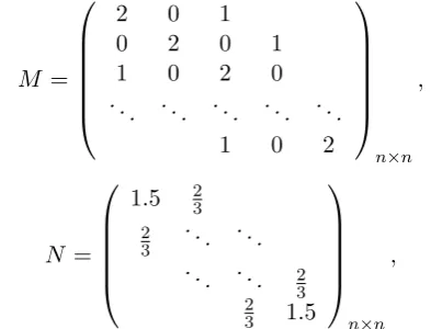
Example 4.1 [20] We consider two HPD matri-ces as follows:
M =
2 0 1
0 2 0 1
1 0 2 0
. .. ... ... ... ...
1 0 2
n×n
,
N =
1.5 23
2
3 . .. ... . .. ... 2
3 2 3 1.5
n×n
,
when n = 100. The results of comparisons for different methods are given in Table 1. In the meantime, we re-examine the above matrices for higher dimensional cases. Results for these cases are gathered up in Tables 2-4.
From the numerical results presented in Tables1
-4, we observe that the accuracy of approximations to the solution increases as the iteration process (2.13) proceed, showing the stable character of the proposed method. The acquired numerical re-sults agree with the theoretical discussions given in the Sections 2-3. The accuracy was measured via (4.30) for this test. Note also that in general the geometric mean of sparse matrices could be dense.
Table4includes a comparison of computational times. Accordingly, we can state that AL2 re-duces the number of iterations and the compu-tational time in finding the geometric mean fa-vorably. The execution time of the new method AL2 in Table 4 seems to grow faster in contrast to NB, thus we expect the latter to be asymptoti-cally better for very large scale matrices. But our proposed algorithm AL2 is a good choice for the moderate sizes. Another point is that although the two methods PM and AL2 are basically the same method applied to different matrices, they achieve much different accuracies in the compu-tation of the geometric mean. This phenomenon occurs since the implementations (structures) of these schemes are totally different to each other as it was seen in Section 2.
∥Y2−Y1∥ ∥Y3−Y2∥ ∥Y4−Y3∥ PM 9.20731 0.0000554761 2.7929×10⁻¹⁴ AL2 8.95253 0.000105972 5.81497×10⁻¹⁴
DB 0.566718 0.126108 0.0608576 NB 80.5 39.2501 17.6667
Table 1: Numerical simulations for Experiment4.1.
∥Y3−Y2∥ ∥Y4−Y3∥ ∥Y5−Y4∥ PM 0.0000554761 2.5209×10⁻¹⁴
AL2 0.000105972 3.85714×10⁻¹⁴
DB 0.126108 0.0608576 0.0218202 NB 39.2501 17.6667 5.84346
Table 2: Results of comparisons for Experiment 4.1
whenn= 200.
∥Y3−Y2∥ ∥Y4−Y3∥ ∥Y5−Y4∥ PM 0.0000554761 2.5209×10⁻¹⁴
AL2 0.000105972 5.712×10⁻¹⁴
DB 0.126108 0.0608576 0.0218202 NB 39.2501 17.6667 5.84346
Table 3: Computational evidences in Experiment4.1
forn= 300.
Example 4.2 In this experiment another exam-ple of different nature has been tested. Let us con-siderM and N to be two Hermitian positive def-inite matrices obtained by taking covariance ma-trix of two random complex matrices of the size
Methods PM AL2 DB NB
n= 100 0.66 0.10 0.56 0.55
n= 150 1.50 0.25 1.20 1.33
n= 200 2.84 0.56 2.19 2.30
n= 250 4.01 1.02 3.60 3.44
n= 300 6.71 1.96 5.07 5.28
n= 350 8.57 3.15 6.70 7.14
n= 400 11.72 6.73 8.82 9.58
n= 450 15.58 9.79 13.06 12.23
n= 500 20.89 13.36 17.25 15.51
n= 550 24.63 17.54 20.25 18.33
n= 600 31.31 21.95 27.69 22.24 Table 4: The elapsed times in Experiment4.1.
●●●●●●●● ● ●●●●●●●●●● ● ●●●●●●●●●●●●●●●●●●●● ●● ● ●●●●●●●●●●●●●●●● ●●●●●●●●●●●●●●●●● ●●● ■■■■■■■■ ■ ■ ■ ■■■■■■■■■■■■■■■■■■■■■■■■■■■■■■■■■■■■■■■■■■■■■■■■■■■■■■■■■■■■■■■■■■■■ ◆◆ ◆◆◆ ◆◆ ◆◆ ◆◆ ◆ ◆◆◆ ◆ ◆◆ ◆◆◆ ◆◆ ◆◆ ◆ ◆◆ ◆◆◆◆◆◆◆◆◆◆◆◆◆◆◆◆◆◆◆◆◆◆◆◆◆◆◆◆◆◆◆◆◆◆◆◆◆◆◆◆◆◆◆◆◆◆◆◆◆◆◆ ▲▲▲▲▲▲▲▲▲▲▲▲▲▲▲▲▲▲▲▲▲▲▲▲▲▲▲▲▲▲ ▲ ▲ ▲ ▲ ▲▲▲ ▲ ▲ ▲ ▲▲▲▲▲▲▲ ▲▲▲▲▲▲▲▲▲▲▲▲▲▲▲▲▲ ▲▲▲▲▲▲▲▲ ▲▲▲▲▲▲▲
20 40 60 80
10-13
10-10
10-7
10-4
10-1
▲ NB
◆ DB
■ AL2 ● PM
Figure 3: Error decay in Experiment4.2.
n = 50; SeedRandom[1];
M = Covariance@RandomComplex[1 + I, {n, n}];
N = Covariance@RandomComplex[2 + I, {n, n}];
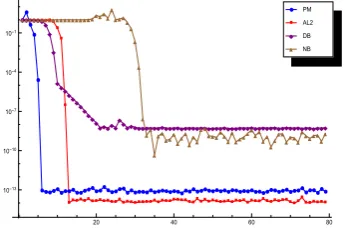
Here, we compare the results of different schemes in Figure 3 in terms of the residual ∥Yk+1−Yk∥∞
∥Yk+1∥∞ after 80 iterations without considering a tolerance to check the stability behavior as well. The quan-tity which is plotted in Figure 3 is ∥Yk+1−Yk∥∞
∥Yk+1∥∞ .
Results are in agreement with the above discus-sions. The interesting point is that only AL2 can reach accuracies higher than 10−9, which is an advantage of the proposed algorithm in contrast to the existing ones.
The higher accuracy of AL2 is due to its high rate of convergence while its computational time is reasonable since the process converges quickly to the matrix geometric mean and this yields in fewer computational effort in the whole of the im-plementation.
Example 4.3 Using the same conditions and criterions as in Experiment4.2, here we compare
the convergence history of different methods for the following two random complex matrices of the size 200×200:
n = 200; SeedRandom[123456]; M = Covariance@RandomComplex[300
- 4 I, {n, n}];
N = Covariance@RandomComplex[ 20, {n, n}];
The results are furnished in Figure 4 in terms of the residual ∥Yk+1−Yk∥∞
∥Yk+1∥∞ .
The results once again show that the presented schemes in this work are good choices for finding the matrix geometric mean of two HPD matrices and they support the theoretical results exposed previously. ● ● ● ● ● ●●●●●●●●●●●●●●●●●●●●●●●●●●●●●●●●●●●●●●●●●●●●●●●●●●●●●●●●●●●●●●●●●●●● ●●●●●● ■■■■■■■■■ ■ ■ ■ ■■■■■■■■■■■■■■■■■■■■■■■■■■■■■■■■■■■■■■■■■■■■■■■■■■■■■■■■■■■■■ ■■■■■■ ◆◆◆◆◆◆◆ ◆ ◆ ◆◆ ◆◆ ◆◆◆ ◆◆ ◆◆ ◆◆◆◆◆ ◆◆ ◆◆◆◆◆◆◆◆◆◆◆◆◆◆◆◆◆◆◆◆◆◆◆◆◆◆◆◆◆◆◆◆◆◆◆◆◆◆◆◆◆◆◆◆◆◆◆◆◆◆◆◆ ▲▲▲▲▲▲▲▲▲▲▲▲▲▲▲▲▲▲▲▲▲▲▲▲▲▲▲▲ ▲ ▲ ▲ ▲ ▲▲ ▲ ▲▲ ▲▲▲▲▲ ▲ ▲ ▲ ▲ ▲▲ ▲▲▲▲▲ ▲ ▲ ▲▲▲ ▲▲▲▲ ▲▲ ▲▲ ▲▲ ▲▲▲▲ ▲ ▲▲▲▲▲▲
20 40 60 80
10-13
10-10
10-7 10-4 10-1 ▲ NB ◆ DB ■ AL2 ● PM
Figure 4: Error decay in Experiment4.3.
5
Conclusion
experiments were furnished. Computational re-sults have justified the effective convergence be-havior of AL2. At last, it is stated that the exten-sion of the new scheme for computing geometric mean of more than two matrices can be taken into account for future works.
References
[1] S. Amat, J. A. Ezquerro, M. A. Hern´ andez-Ver´on, On a new family of high-order itera-tive methods for the matrixpth root,Numer. Linear Algebra Appl.22 (2015) 585-595.
[2] R. Bhatia, Positive definite matrices, Prince-ton Series in Applied Mathematics, Prince-ton University Press, PrincePrince-ton,(2007).
[3] E. Denman, A. Beavers, The matrix sign function and computations in systems,Appl. Math. Comput.2 (1976), 63-94.
[4] A. Frommer, B. Hashemi, T. Sablik, Com-puting enclosures for the inverse square root and the sign function of a matrix,Linear Al-gebra Appl.456 (2014) 199-213.
[5] O. Gomilko, D. B. Karp, M. Lin, K. Zi¸etak, Regions of convergence of a Pad´e family of iterations for the matrix sector function and the matrixp-th root, J. Comput. Appl. Math.236 (2012) 4410-4420.
[6] F. Greco, B. Iannazzo, F. Poloni, The Pad´e iterations for the matrix sign function and their reciprocals are optimal,Linear Algebra Appl.436 (2012) 472-477.
[7] N. J. Higham, The matrix sign tion and its relation to the polar decomposi-tion,Lin. Algebra Appl. 212 (1994) 3-20.
[8] N. J. Higham, Accuracy and Stability of Nu-merical Algorithms, Second Edition, SIAM, UK,2002.
[9] N. J. Higham, Functions of Matrices: The-ory and Computation,Society for Industrial and Applied Mathematics, Philadelphia, PA, USA,2008.
[10] B. Iannazzo, The geometric mean of two matrices from a computational view-point,Numer. Linear Algebra Appl.23 (2016) 208-229.
[11] C. S. Kenney, A. J. Laub, Rational iterative methods for the matrix sign function,SIAM J. Matrix Anal. Appl.12 (1991) 273-291.
[12] F. Khaksar Haghani, F. Soleymani, An im-proved Schulz-type iterative method for ma-trix inversion with application, Tran. Inst. Measur. Cont.36 (2014) 983-991.
[13] D. Li, P. Liu, J. Kou, An improvement of Chebyshev-Halley methods free from second derivative, Appl. Math. Comput. 235 (2014) 221-225.
[14] T. Lotfi, F. Soleymani, M. Ghorbanzadeh, P. Assari, On the construction of some tri-parametric iterative methods with memory,
Numer. Algorithms 70 (2015) 835-845.
[15] J. D. Lawson, Y. Lim, The geometric mean, matrices, metrics and more, Amer. Math. Month.108 (2001) 797-812.
[16] M. Sh. Misrikhanov, V. N. Ryabchenko, Ma-trix sign function in the problems of analysis and design of the linear systems, Auto. Re-mote Cont. 69 (2008) 198-222.
[17] G. Pusz, S. L. Woronowicz, Functional calcu-lus for sesquilinear forms and the purification map, Rep. Math. Phys.8 (1975) 159-170.
[18] F. Soleymani, E. Tohidi, S. Shateyi, F. Khaksar Haghani, Some matrix iterations for computing matrix sign function,J. Appl. Math.(2014) 9 pages.
[19] F. Soleymani, P. S. Stanimirovi´c, I. Sto-janovi´c, A novel iterative method for po-lar decomposition and matrix sign function,
Disc. Dyn. Nat. Soc.(2015).
[21] J. L. Varona, Graphic and numerical com-parison between iterative methods, Math. Intell.24 (2002) 37-46.
[22] Wolfram Research, Inc., Mathematica, Ver-sion 10.1,Champaign, IL (2015).